Featured Application
This work can be potentially valuable to be used as a reference for existing estimating methods based on NDT.
Abstract
A pressurized spherical shell that is continuously corroded will likely buckle and lose its stability. There are many analytical and numerical methods to study this problem (critical load, critical thickness, and service life), but the friendliness (operability) in engineering test applications is still not ideal. Therefore, in this paper, we propose a new non-destructive method by combining the Southwell non-destructive procedure with the stable analysis method of corroded spherical thin shells. When used carefully, it can estimate the critical load (critical thickness) and service life of these thin shells. Furthermore, its procedure proved to be more practical than existing methods; it can be easily mastered, applied, and generalized in most engineering tests. When used properly, its accuracy is acceptable in the field of engineering estimations. In the context of the high demand for non-destructive analysis in industry, it may be of sufficient potential value to be used as a reference for existing estimating methods based on NDT data.
1. Introduction
Due to the increasing use of shell-type structures in spacecrafts, submarines, buildings, and storage tanks, there has been a corresponding increase in the interest of researchers and practical engineers in the stability of shells. Hemispherical shells are the most important structural element in engineering applications because they can resist higher pure internal pressure loads than any other geometric vessel with the same wall thickness and radius.
In practice, most pressure vessels experience external loads due to hydrostatic pressure or external shocks-. Therefore, they should be designed to withstand the worst load combinations without failure. Loads transmitted by cylindrical rigid actuators applied on top of the sphere are considered common external loads. Therefore, it is important to study its effect on the initial buckling behaviour of such shells. Meanwhile, corrosion is defined as the gradual destruction of a material due to chemical reactions within the environment. The most common type of corrosion is uniform corrosion or general corrosion, which is distributed almost uniformly over the entire exposed surface. General wear can occur both with the formation of a fully protective ultra-thin coating of corrosion products and without an oxide layer. The formation of a blocking passivation film, as well as changes in the concentration of one or the other reactants, may inhibit when the corrosion rate should decay exponentially (decline) with time [1,2,3].
On the other hand, as with other types of damage (e.g., [4]), corrosion can be enhanced by the applied load [5]. Experimental data suggests that there is a stress corrosion threshold, after which mechanical stress accelerates corrosion [5,6,7]. In this case, the stress changes due to the reduction in shell thickness, and the changed stress in turn enhances the corrosion process. In general, for the strength analysis of structural elements under mechano-chemical corrosion conditions, an initial boundary value problem with unknown evolutionary boundaries must be solved.
In addition to stress, there are many other effects that can affect the corrosion rate, such as temperature; it has a great influence on the rate of galvanic corrosion of metals. In the case of neutral-solution corrosion (oxygen depolarization), elevated temperature has a favourable effect on the overpotential and oxygen diffusion rate for oxygen depolarization but leads to a decrease in oxygen solubility. When corrosion (hydrogen depolarization) occurs in acidic media (such as sea water), the corrosion rate increases exponentially with increasing temperature due to the reduced hydrogen evolution overpotential. An Arrhenius-type experimental dependence was observed between corrosion rate and temperature [8]. The effect of temperature on acid corrosion, most commonly in hydrochloric and sulfuric acid, has been the subject of extensive research [9,10,11,12,13,14,15,16,17,18,19,20,21,22]. In hydrochloric acid, the effective activation energies for corrosion processes vary from 57.7 to 87.8 kJ mol/L, where most are concentrated around 60.7 kJ mol/L. In some cases, studies were performed at only three temperature values using a single experimental method, which increased the likelihood of erroneous determination of the corrosion activation energy. In this regard, further research is advisable, as it may provide a reliable comparative basis for discussing the obtained results.
In summary, we know that temperature has a great influence on corrosion rate, corrosion and stress can interact with each other, and finally, they can jointly affect the stability of the shell. In this regard, we should explore the relationships of temperature, corrosion, and stress to shell stability. Experimental [23], analytical [24,25,26,27,28], and numerical methods [29,30,31] were used to study the buckling of (uniformly compressed hemispherical of moderate thickness) metal shells using corrosion and temperature. A related study [28] also demonstrated the high accuracy of these methods. However, in practical engineering applications, they often lack operability and are less friendly to workers.
Non-destructive estimation methods, such as in the field of pressure vessels, have been a research hotspot due to their advantages of simple operation, widespread use, and low cost. As one of the non-destructive methods, the non-destructive approach of Southwell’s column analysis is now extended to spherical shells, which are subjected to uniform external pressure [32]. However, there are few non-destructive methods for estimating the buckling of pressure spherical shells of this type. The paper [33] established a non-destructive estimation method for a spherical shell under external pressure that can predict its critical load. It is based on an exact first-order solution of the critical stress and requires two assumptions: one is that the thickness of the shell does not change; and the second is that the temperature does not affect the critical buckling of the shell. In any case, when the shell is in a corrosive environment, the thickness of the shell varies and the effect of temperature on both the stress and the corrosion rate is unavoidable. No non-destructive method has been found as of yet to predict the critical loads (stresses) of the shell under this condition, including the service life. Therefore, in the industry, people still hope to obtain a new lossless method. This method can predict the critical load (or stress) and critical thickness of the shell under external pressure from corrosion on the basis of a higher-order (second-order) exact solution. At the same time, we are also oriented to predict its useful (remaining) life. For this reason, in this paper, we will analytically extend the Southwell process method for the non-destructive prediction of critical loads, critical stresses, and service life of hemispherical shells subjected to uniform external pressure considering corrosion and ambient temperature through rigorous mathematical derivation.
2. Problem Description
A model of a spherical shell is considered. It is affected by the external pressure po, and its inner surface undergoes mechano-chemical corrosion, as shown in Figure 1. Assuming that the rate of internal corrosion is vo, the corrosion process causes the thickness h of the shell to change with time t. We adopt the effective stress definition to characterize stress here, which is commonly used when corrosion is present.
Figure 1.
A spherical shell subjected to both external pressure and internal corrosion.
The problem in this paper is to predict (estimate) the critical thickness, critical stress, and service life of the spherical shell based on non-destructive testing data in a temperature and corrosive environment. This is essentially a non-destructive estimation problem involving variable boundary conditions. For clarity, we describe this complex and combined problem in two steps.
2.1. Before All, It Is Necessary to Solve the Estimation of the Critical Thickness, Critical Stress, and Service Life of the Shell Based on NDT Data in a Non-Corrosion and Temperature-Independent Environment
It involves two sub-problems. First, theoretically, we need to obtain the second-order buckling critical stress for the spherical shell model (see Appendix A), which is the accurate solution. Then, based on the format of this second-order solution, a test data-based estimation method for the shell critical stress will be established by introducing an existing non-destructive method (see [33]).
The mathematical problem involved in obtaining the second-order buckling critical stress is related to the solution of the following Equations (1)–(4):
where u is the displacement of the shell element in x direction, v is the displacement in y direction, w is the displacement in z direction, t0 is the shell thickness, pcr is the classical buckling pressure, , are the resultant forces, Qx, Qy are the shear forces, Mx, My are the bending moments, and , are the angles of the shell element.
When introducing the non-destructive method, the corresponding mathematical problem involved is how to express the relationship between non-destructively measurable quantities (such as: w and w/p at any point on the outer surface of the shell) as an equation of a straight line. The physical quantity to be estimated (e.g., the critical load pcr of the shell) needs to appear exactly in the expression of the line slope. Assuming that we can obtain this equation line by non-destructive testing in the elastic stage, the quantity to be estimated can be obtained immediately. For example, let us take Equation (12) in which the equation slope is . Then suppose we get the slope by testing and drawing; therefore, the only unknown quality in it, , can be expressed (obtained) by the slope easily.
Moreover, the assumptions within this non-destructive method are that the shell deformation is axisymmetric and the compression in the shell is uniform. At the same time, it does not assume the specific location of buckling and the number of buckling waves, as shown in Figure 2.
Figure 2.
The non-destructive method does not assume the exact location of spherical shell buckling (e.g., the point M or N) and the number of buckling waves.
2.2. Then, on the Basis of the Previous Step 2.1, We Can Further Solve the Problem of Critical Load (Stress) and Service Life in an Environment Where Corrosion and Temperature Coexist
The mathematical problem that needs to be solved is similar to that in Section 2.1, but an extra equation (corrosion kinetic equation) needs to be taken into consideration—the relationships between the corrosion rate (that is, the derivative of thickness), temperature, and stress:
here, for f (σ, T) we adopt:
where h is the thickness of the shell, t is the corrosion time, is the initial corrosion rate, is the stress, T is the temperature, is the molar gas constant, and V is the material molar volume.
It is noted that the derivation process of Equation (6) is shown in Appendix B, where we found that the relationship between corrosion rate and temperature conforms to the Arrhenius type [5]. Meanwhile, it should be observed that according to the physical definition of shell buckling, the critical thickness in the case described in this section will be identical to its expression obtained in Section 2.1.
3. Problem Solving
In order to solve the problems highlighted in this paper (see Section 2), we run the following two steps to explain our methods.
3.1. First Step: Establish a Non-Destructive Method for Predicting Spherical Shell Life Regardless of Corrosion and Temperature
From (A50) in Appendix A.1, we rewrite the it as:
Here, m is the ratio of the thickness to the radius of the sphere.
We rewrite Equation (A51) in Appendix A.1 as:
here, .
Let , from Equations (7) and (8), we can obtain:
and then
By substituting Equation (10) into Equation (A69) in Appendix A.2, we get:
As can be seen from the equations above, we have successfully established the relationship between the displacement and the pressure of the shell by appropriately rewriting the form of the second-order critical load and combining the relationship between the displacement w and the rotation angle φ shown in Equation (5).
By cross-multiplying in Equation (11), we can achieve:
Formally, Equation (12) is the equation of a straight line following the Southwell procedure described in Section 2.1. It has w as one axis and w/p as another. Furthermore, the expression of the slope of this line contains the unknown critical load pcr. Therefore, the slope of this line can be gained experimentally, and the critical load can then be obtained.
Let ; Equation (12) can be rewritten as:
one can get:
By substituting Equation (A53) in Appendix A.1 into Equation (7), we get:
With the previous steps, we have obtained a non-destructive estimation of the critical thickness (see Equation (18)) in the same way that we have used to solve the critical load above (see Equation (14)).
3.2. Second Step: Establish a Non-Destructive Method for Predicting Critical Load, Critical Thickness, and Service Life of Spherical Shells in the Presence of Corrosion and Temperature
According to the description in Section 2.2, this case requires an additional corrosion-rate equation than in Section 2.1—see (A77) in Appendix B.
Considering Equation (10), from Equation (A77) we obtain:
Through performing variable separation on Equation (19) in we get:
where, t0 refers to the initial time, t* to the service life, σ0 to the stress at time t0, and σ* to the critical stress.
Integrating Equation (20), we get:
Considering that Equation (10) establishes consistency, through , the service life t* can be obtained:
If we still consider Equation (10), Equation (A77) can be transformed into:
In order to separate the variables t and h in [t0, t*] and [h0, h*], first we get:
then:
and finally:
Note that in this section we still have , , and .
4. Example Analysis
The whole process described above (including those in Appendix A and Appendix B), showed that the non-destructive method of this paper used mathematical logic rigorously. To further validate it, we compare its results with those of other methods on this section. Due to the limitation of NDT data found in literature on these kinds of shells, we compare our method within a special case in Section 2.1 (without corrosion and temperature) with another existing method.
The NDT data adopted here is taken from an experiment described in [33]. To maintain consistency with the experimental model of [33], we also apply internal suction to our FE model to simulate equivalently the external pressure. The geometric parameters for the FE model (meeting thin wall hypothesis) are: the radius of shell r = 0.05 m and the wall thickness h0 = 0.0005 m, yielding a h0/r ratio of 0.01. The mechanical properties are: the Young modulus E = 650 MPa, Poisson ratio ν = 0.4, and density ρ = 1150 kg/m3.
A 1/8 symmetrical spherical shell model built by the ANSYS software is shown in Figure 3. The first two buckling modes obtained from the eigenvalue buckling analysis are shown in Figure 4.
Figure 3.
1/8 symmetrical spherical shell FE model.
Figure 4.
Buckling modes obtained from the eigenvalue buckling analysis.
First, we calculate the value of using the described method. The results for w and w/p are plotted in Figure 5.
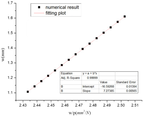
Figure 5.
Plot of w/p vs. w (R = 50 mm, h = 0.5 mm).
Within the plot, it is shown that the fitting line equation for the w and w/p points is:
therefore, we get S = 7.27385 by Equation (13), and then obtain = 0.08593 through Equation (14).
w + 7.27385 w/p = 16.59268,
In order to verify the practicality and accuracy of this method, we also calculate the value adopting the other five existing methods, including one-order analytical value, numerical value, two-order analytical value, etc., which are shown in Table 1. The highest error is produced from the numerical method of [33], while the lowest error is produced from the lowest eigenvalue method.

Table 1.
Critical load of our method comparing with other methods.
Because the error values from our method, when used correctly, are within the range of the other approaches, its accuracy can be considered acceptable in the field of engineering. Besides that, compared with other methods, there is no doubt that our method is the most practical and easiest one to operate in engineering.
From Table 1, we also note that the experimental values are the smallest relative to any other method (numerical methods of various orders, analytical methods, etc.). There may be several reasons to explain this behavior: for example, the roundness of the actual shell (not ideal), but with geometric imperfections; also, the realistic boundary support is not a 100%-hinged support or a 100%-fixed support either. However, we use the 100%-hinged support in the numerical model for simplification.
5. Practical Implementation of This Method
This method is friendly to inspectors working for practical projects and easy to implement. Its general steps are as follows: basically, we should apply an external uniform pressure (or equivalent uniform pressure) p by n times to the shell. Here, = + , i = 1, 2, 3, …, n. At the same time, we record the deformation after each loading. Here, the parameter S can be obtained through Equation (13). Then the is obtained by Equation (14). Then by the same way, we can obtain parameter J by Equation (17), and accordingly obtain by Equation (18), and finally obtain by Equation (26).
6. Conclusions
The highlight of this study is that it proposes a non-destructive method based on the Southwell procedure to estimate the critical load, critical thickness, and service life of internally corroded shells under external pressure while considering the temperature’s effect. Of course, it is also applicable for the shell in special cases, such as industrial environments without corrosion or temperature.
Based on rigorous theories (shell stability theory, the Southwell plot method, and corrosion dynamic theory), and following a scientific route from simple to complex, we derived and acquired our new method step-by-step. We first derived the critical load and critical thickness of the spherical shell in the absence of corrosion and temperature using the Southwell procedure method. Second, we derived non-destructive methods for critical load, critical thickness, and service life prediction under corrosion and temperature conditions. Third, we compared our method with other methods.
The results show that, if used properly, engineering precision requirements can be met. Furthermore, when the results are carefully interpreted, this technique provides useful estimates of elastic buckling loads (critical thickness and service life). The utility of this approach lies in the fact that it is versatile, simple, and non-destructive. Furthermore, it does not require any assumptions about the buckling wave number or the precise location of buckling.
It has to be pointed out that since the service life of a spherical shell is usually very long (and so is its corrosion process), NDT data for the shells that are regularly detected, especially those collected regularly during the shell corrosion process, and fully recorded and published data, has not been found. A very small part of it was found in some data from experiments, which is employed in this paper in Section 4. This is why the method in this paper cannot be successfully verified in more working conditions currently. However, the authors will try to obtain (retrieve data from peer industries) NDT data under more operating conditions to fully evaluate the non-destructive prediction ability of this method for the shell service life (such as serving in corrosive and temperature environments) in the near future.
In summary, the highlight of this method in evaluating critical loads (thickness, lifetime) for shells is that it is non-destructive. Additionally, it is the first time introducing the Southwell plot method into the stabilization analysis of shells of time-varying thickness. Its precision meets engineering requirements, and more importantly, it is practice- and implementation-friendly.
Author Contributions
Conceptualization, methodology, software, validation, formal analysis, C.H.L. Investigation; resources; data curation; writing—review and editing, visualization, supervision, funding acquisition, G.L. All authors have read and agreed to the published version of the manuscript.
Funding
This work was supported by the National Natural Science Foundation of China [Grant number, 52068003] and by the Opening Project of Guangxi Laboratory on the Study of Coral Reefs in the South China Sea, China [Grant number, GXLSCRSCS201900*]. Moreover, the sponsorship guaranteed with basic research funds provided by Politecnico di Torino (Italy) is acknowledged. Opinions, findings, and conclusions expressed in this paper are those of the authors and not necessarily those of the sponsors. The author C.H.L. also acknowledges funding for the Training Program of 1000 Young and Middle-aged Outstanding Teachers in Colleges and Universities from Guangxi Education Department (CED) of China (No.: t2010097921).
Institutional Review Board Statement
Not applicable.
Informed Consent Statement
Not applicable.
Data Availability Statement
Available when asked for academic use.
Acknowledgments
The author (C.H.L.) is thankful to the Department of Mathematics for hospitality during her stay at Aberystwyth University. The authors (C.H.L. & G.L.) thank H. Yuan in USA and H. Nunn in Aberystwyth University for fruitful discussions. The author (C.H.L.) also thanks S. Shi in the Department of Mathematics of Hefei University of Technology, S. Huang and I. Burgess in the Department of Civil and Structural Engineering of the University of Sheffield for discussing in its earlier stage.
Conflicts of Interest
The authors declare no conflict of interest.
Notation List
| S | slope of w vs. w/p line |
| u | displacement of the shell element in x direction |
| v | displacement of the shell element in y direction |
| w | displacement of the shell element in z direction |
| U0 | effect of initial imperfections |
| V | shearing force in straight members in y direction (buckling coefficient to be determined experimentally) |
| unit elongation or strain in x-direction | |
| unit elongation or strain in y-direction | |
| unit elongation of middle surface in x-direction | |
| unit elongation of middle surface in y-direction | |
| Poisson’s ratio | |
| change of curvature in x-direction | |
| change of curvature in y-direction | |
| t0 | thickness of the shell |
| pcr | buckling pressure |
| H( ) | mathematical operator |
| Nx, Ny | resultant forces |
| Qx, Qy | shear forces |
| Mx | My bending moments |
| po | outer pressure |
| vi | inner mechano-chemical corrosion rate |
| t | time |
| h | thickness |
| σ | principal stress |
| σe | effective stress |
| r | distance between a point in the shell material and the origin of the coordinate system/radius of two concentric spheres |
| ro | distance between the point in the outer shell surface and the origin of the coordinate system |
| b | corrosion inhibition effect |
| dr | radius of two concentric spheres |
| dθ, dφ | top angles of four wedge-shaped sections |
| rc | midsurface radius |
| x | thickness to midsurface radius ratio |
| t* | time required for a corroded pressure shell to fail for the first time due to buckling or yielding |
| h | corresponding thickness of the shell under the critical failure state |
Appendix A. Buckling Formulas for Spherical Shells in the Case of Section 2.1 (without Corrosion and Temperature)
Appendix A.1. Derivation of the Second-Order Critical Buckling Load (Stress)

Figure A1.
Hemispherical shells and one-half analysis model.
Figure A1.
Hemispherical shells and one-half analysis model.


Figure A2.
Hemispherical shell element and corresponding forces.
Figure A2.
Hemispherical shell element and corresponding forces.

Using the above derived angles instead of the initial ones,, and , the equations of equilibrium of the element ABCD become [33]:
w + 7.27385 w/p = 16.59268,

Figure A3.
Meridian of a spherical shell before and after buckling.
Figure A3.
Meridian of a spherical shell before and after buckling.

Here, u is the displacement of the shell element in x direction, v is the displacement of the shell element in y direction, w is the displacement of the shell element in z direction, t0 is the thickness of the shell, pcr is the classical buckling pressure, Nx, Ny are the resultant forces, Qx, Qy are the shear forces, Mx, My are the bending moments, and , are the angles of the shell element.
If a spherical shell is submitted to a uniform external pressure, there will be a uniform compression whose magnitude is:
Let ,, and represent the components of small displacements during buckling from the compressed spherical form, then and differ little from the uniform compressive force and become:
where and are the resultant forces due to small displacements , and .
Due to the stretching of the surface, becomes Therefore, substituting Equations (A5) and (A6) back into the differential equations of equilibrium (A1), (A2), and (3), and simplifying and neglecting the small terms, such as the products of , and with the derivations of , and , we obtain:
From Equation (A9) we get:
Substituting into the Equations (A7) and (A8), and considering the following equations:
together with:
Here, the unit elongation or strain in the x-direction, is the unit elongation or strain in the y-direction, is the unit elongation of middle surface in the x-direction, is the unit elongation of middle surface in the y-direction, is Poisson’s ratio, is the change of curvature in the x-direction, and is the change of curvature in the y-direction.
Then they can be written as:
And then we get:
Now, introducing two dimensionless parameters, and —which are defined as and —and using the elastic law to express the forces and moments in terms of and one obtains the differential equations of equilibrium ((A7) and (A8)):
These two equations may be simplified by neglecting, in comparison with unity, the first term, since the shell is thin, and therefore, the ratio is very small. Moreover, due largely to angular displacement , we make good use of this situation by introducing an auxiliary variable u, such that .
Thus, the expressions in the brackets in Equation (A29) become identical. Then, using the mathematical operator , it turns to:
The fourth term, containing the factor, may be neglected in comparison with the third in Equation (A31). Integrating the Equation (A31) with respect to and assuming that the constant of integration is equal to zero, we obtain:
Now, any regular function of in the interval may be expanded in a series of Legendre functions:
in which , and is an integer.
Assuming the general expressions of and for any symmetrical buckling of spherical shells, we have:
Substituting them back to Equations (A35) and (A36), we can have:
The Legendre functions form a complete set of functions. Therefore, the two series cannot vanish identically unless each coefficient vanishes.
From Equation (A29) we can get:
and eliminating from the above set of equations, Equation (A41) can then be written as:
Buckling of the shells becomes possible if these equations, for some value of n, yield for An and Bn a solution different than zero, which means a trivial solution; in other words, having a zero determinant of the system of equations. Thus:
a solution of which is , which corresponds to a value of n equals to unity. Substituting this value of into Equation (A40), one obtains:
Now, for , other than zero:
which yields for its minimum, or for after simplification:
and yields the first critical load [33]:
Equation (A51) was derived with the assumption that the shell wall thickness is specified, whereas the critical value of external pressure Q is the unknown quantity.
On the contrary, if we assume that the external pressure Q value is specified, then the shell wall thickness h*, corresponding to the stability loss, will be equal to:
Appendix A.2. Derive the Relationship between w and φ of the Spherical Shell
In 1934, Southwell began using his approach on columns. In this part of the section, an attempt is made to demonstrate that uniformly compressed spherical shells can also be analyzed by the Southwell procedure. In the derivation of the formula, as it was done for the classical theory of buckling shells (see previous part), it is assumed that the displacements and may be expressed as [33]:
where is the Legendre functions of the orders , while and are the real constants from before:
Additionally, it is assumed that the manufacturing imperfections of is equal to zero. Thus, it is tried only with the direction .
When the compressive load p is applied to the shell, each point of the middle surface undergoes elastic displacements and , and its normal distance from the reference sphere then becomes . It is assumed that is from the order of the elastic deformation, and then the element of the shell looks like the deformed elements, which are used to establish the differential equations of the buckling problem. Again, going through the same procedure, one finds that the terms of those equations belong to two groups (see the proceeding section). In those terms, which contain the factor , the quantities and describe the difference in shape between the deformed element and an element of a true sphere. In these terms, w must now be replaced by . On the other hand, all terms that do not have the factor , can be traced back to terms of the elastic law, and represent the stress resultants acting on the shell element. Before the application of the load, the shell is free of stress, and the stress resultants depend only on the elastic displacements u and w. Consequently, in all these terms, w does not need to be replaced by , but stays w.
Thus, one arrives at the following set of differential equations:
in which denotes the same operator as before:
Thus, the problem is reduced to solving this set of equations. Eliminating from the above set of equations:
After canceling and neglecting the small quantities as ,, and their products in comparison with unity, we obtain:
Coming back to the definition of the displacement w, one may write the equation —or writing it in detail:
here , which is the minimum for ; therefore, it has the same values for n equals to minus one and zero. Since n must be an integer, it is chosen as zero, which yields , and corresponds to , which is a function of , and gets smaller when becomes greater. Thus, it is possible to neglect all the terms and simply write since the terms which contain ,… are much smaller—so, buckling is usually expected at the places where is large [33]:
Appendix B. Deriving the Corrosion Rate of the Spherical Shell as a Function of Temperature and Stress, Based on the Arrhenius Type
It is assumed that the shell is subjected to the simultaneous action of a constant external pressure Q and uniform internal corrosion. The rate of the thickness decrease at each moment of time t is equal to the corrosion rate [5]:
where is a sufficiently smooth function of compressive stress , defined by Equation (A2), and the temperature . The corrosion rate dependence on the stress value, according to experimental data, can be approximated by exponential function suggested in [1], while the temperature effect is usually described by the Arrhenius-type law [11]. Combination of both functions yields the following relation Equation (A73).
Temperature has a great effect on the rate of metal electrochemical corrosion. In the case of corrosion in a neutral solution (oxygen depolarization), the increase of the corrosion rate increases exponentially with temperature increase because the hydrogen evolution overpotential decreases. Experimental dependence of the Arrhenius type is observed between the corrosion rate and temperature. Using the current density , we express the corrosion rate [1]:
where is the effective activation energy of the corrosion process in kJ mol−1, the molar gas constant in J mol−1 K−1, T is the absolute temperature in K, the pre-exponential factor, and the corrosion current density, A cm−2. Equation (A71) provides the determination of the effective activation energy of the corrosion process.
When , we have and .
Moreover, when , , and we get:
Considering [1], and then using linear scale method, we get:
From the above equation, we know:
therefore, we can easily get:
and thus:
Finally, we have [5]:
in which is the molar gas constant, V is the material molar volume, , and .
References
- Li, L.; Gao, J.; Wang, Y. Evaluation of cyto-toxicity and corrosion behavior of alkali-heat-treated magnesium in simulated body fluid. Surf. Coat. Technol. 2004, 185, 92–98. [Google Scholar] [CrossRef]
- Ben Seghier, M.E.A.; Höche, D.; Zheludkevich, M. Prediction of the internal corrosion rate for oil and gas pipeline: Implementation of ensemble learning techniques. J. Nat. Gas Sci. Eng. 2022, 99, 104425. [Google Scholar] [CrossRef]
- Islam, M.A. Corrosion behaviours of high strength TMT steel bars for reinforcing cement concrete structures. Procedia Eng. 2015, 125, 623–630. [Google Scholar] [CrossRef]
- Páczelt, I.; Kucharski, S.; Mróz, Z. The experimental and numerical analysis of quasi-steady wear processes for a sliding spherical indenter. Wear 2012, 274–275, 127–148. [Google Scholar] [CrossRef]
- Gutman, E.M. Mechanochemistry of Solid Surfaces; World Scientific Publishing Company: Singapore, 1994. [Google Scholar] [CrossRef]
- Kashani, M.M.; Crewe, A.J.; Alexander, N.A. Nonlinear stress-strain behaviour of corrosion-damaged reinforcing bars including inelastic buckling. Eng. Struct. 2013, 48, 417–429. [Google Scholar] [CrossRef]
- Möller, B.; Albrecht, S.; Wagener, R.; Melz, T. Fatigue strength of laser beam welded steel-aluminium joints considering variable amplitude loading and corrosive environment. Procedia Struct. Integr. 2019, 18, 556–559. [Google Scholar] [CrossRef]
- Popova, A.; Sokolova, E.; Raicheva, S.; Christov, M. AC and DC study of the temperature effect on mild steel corrosion in acid media in the presence of benzimidazole derivatives. Corros Sci. 2003, 45, 33–58. [Google Scholar] [CrossRef]
- Tanveer, N.; Mobin, M. Corrosion Protection of Carbon Steel by Poly (aniline-co-o-toluidine) and Poly (pyrrole-co-o-toluidine) Copolymer Coatings. J. Miner Mater. Charact. Eng. 2011, 10, 735–753. [Google Scholar] [CrossRef]
- Noor, E.A. Temperature effects on the corrosion inhibition of mild steel in acidic solutions by aqueous extract of fenugreek leaves. Int. J. Electrochem. Sci. 2007, 2, 996–1017. [Google Scholar]
- Al-Majedy, Y.K.; Ibraheem, H.H.; Falih, M.S.; Al-Amiery, A.A. New coumain derivatives as corrosion inhibitor. IOP Conf. Ser. Mater. Sci. Eng. 2019, 579, 012051. [Google Scholar] [CrossRef]
- Abdel-Azim, A.A.; Milad, R.; El-Ghazawy, R.; Kamal, R. Corrosion inhibition efficiency of water soluble ethoxylated trimethylol propane by gravimetric analysis. Egypt J. Pet. 2014, 23, 15–20. [Google Scholar] [CrossRef]
- AL-Saadie, K.; Abdul Karime, N.; Al-Mousawi, I.M. Corrosion Inhibition of Zinc in Hydrochloric Acid Medium Using Urea Inhibitor. J. Al-Nahrain Univ. Sci. 2007, 10, 31–38. [Google Scholar] [CrossRef]
- Patil, D.B.; Sharma, A.R. Study on the corrosion kinetics of iron in acid and base medium. E-J. Chem. 2011, 8 (Suppl. 1), 358–362. [Google Scholar] [CrossRef]
- Zhang, H.H.; Qin, C.K.; Chen, Y.; Zhang, Z. Inhibition behaviour of mild steel by three new benzaldehyde thiosemicarbazone derivatives in 0.5 M H2SO4: Experimental and computational study. R. Soc. Open Sci. 2019, 6, 190192. [Google Scholar] [CrossRef]
- Nicol, M.J. A comparative study of the kinetics of the oxidation of iron(II) by oxygen in acidic media - mechanistic and practical implications. Hydrometallurgy 2020, 192, 105246. [Google Scholar] [CrossRef]
- Hashim, N.Z.N.; Kassim, K. The effect of temperature on mild steel corrosion in 1 M HCL by Schiff bases. Malaysian J. Anal. Sci. 2014, 18, 28–36. [Google Scholar]
- Solutions, I.A. Electrodissolution Kinetics of Iron and Its Alloys Containing Titanium in Chloride Solutions. 1975. Available online: https://core.ac.uk/download/pdf/147423716.pdf (accessed on 31 October 2022).
- Gao, M.; Wang, H.; Song, Y.; Han, E.H. Corrosion behavior on carbon steel in a simulated soil solution under the interaction effect of chloride and bicarbonate ions. J. Mater. Res. Technol. 2022, 21, 3014–3024. [Google Scholar] [CrossRef]
- Piatti, R.C.V.; Arvía, A.J.; Podestá, J.J. The electrochemical kinetic behaviour of nickel in acid aqueous solutions containing chloride and perchlorate ions. Electrochim. Acta 1969, 14, 541–560. [Google Scholar] [CrossRef]
- Fassina, P.; Bolzoni, F.; Fumagalli, G.; Lazzari, L.; Vergani, L.; Sciuccati, A. Influence of hydrogen and low temperature on mechanical behaviour of two pipeline steels. Eng. Fract. Mech. 2012, 81, 43–55. [Google Scholar] [CrossRef]
- Garrigues, L.; Pebere, N.; Dabosi, F. An investigation of the corrosion inhibition of pure aluminum in neutral and acidic chloride solutions. Electrochim. Acta 1996, 41, 1209–1215. [Google Scholar] [CrossRef]
- Colacino, E.; Carta, M.; Pia, G.; Porcheddu, A.; Ricci, P.C.; Delogu, F. Processing and Investigation Methods in Mechanochemical Kinetics. ACS Omega 2018, 3, 9196–9209. [Google Scholar] [CrossRef] [PubMed]
- Bergman, R.M.; Levitsky, S.P.; Haddad, J.; Gutman, E.M. Stability loss of thin-walled cylindrical tubes, subjected to longitudinal compressive forces and external corrosion. Thin-Walled Struct. 2006, 44, 726–729. [Google Scholar] [CrossRef]
- Gutman, E.M.; Bergman, R.M.; Levitsky, S.P. Influence of internal uniform corrosion on stability loss of a thin-walled spherical shell subjected to external pressure. Corros. Sci. 2016, 111, 212–215. [Google Scholar] [CrossRef]
- Gutman, E.; Haddad, J.; Bergman, R. Stability of thin-walled high-pressure vessels subjected to uniform corrosion. Thin-Walled Struct. 2000, 38, 43–52. [Google Scholar] [CrossRef]
- Elso, M.I. Finite Element Method studies on the stability behavior of cylindrical shells under axial and radial uniform and non-uniform loads. Master’s Thesis, University of Applied Sciences, Krefeld, Germany, May 2012. [Google Scholar]
- Wang, H.; Zhu, Y.; He, X.; Guan, W.; Zhan, M.; Zhang, J. Strength Prediction of Spherical Electronic Cabins with Pitting Corrosion. Metals 2022, 12, 1120. [Google Scholar] [CrossRef]
- Naseri Ghalghachi, R.; Showkati, H.; Eyvazinejad Firouzsalari, S. Buckling behaviour of GFRP cylindrical shells subjected to axial compression load. Compos. Struct. 2021, 260, 113269. [Google Scholar] [CrossRef]
- Amaya-Gómez, R.; Sánchez-Silva, M.; Bastidas-Arteaga, E.; Schoefs, F.; Muñoz, F. Reliability assessments of corroded pipelines based on internal pressure—A review. Eng. Fail. Anal. 2019, 98, 190–214. [Google Scholar] [CrossRef]
- De Meo, D.; Oterkus, E. Finite element implementation of a peridynamic pitting corrosion damage model. Ocean Eng. 2017, 135, 76–83. [Google Scholar] [CrossRef]
- Do, V.D.; Le Grognec, P.; Rohart, P. Closed-form solutions for the elastic—Plastic buckling design of shell structures under external pressure. Eur. J. Mech. A Solids 2023, 98, 104861. [Google Scholar] [CrossRef]
- Nayyeri Amiri, S.; Rasheed, H.A. Nondestructive method to predict the buckling load in elastic spherical shells. Eng. Struct. 2017, 150, 300–317. [Google Scholar] [CrossRef]


Disclaimer/Publisher’s Note: The statements, opinions and data contained in all publications are solely those of the individual author(s) and contributor(s) and not of MDPI and/or the editor(s). MDPI and/or the editor(s) disclaim responsibility for any injury to people or property resulting from any ideas, methods, instructions or products referred to in the content. |
© 2023 by the authors. Licensee MDPI, Basel, Switzerland. This article is an open access article distributed under the terms and conditions of the Creative Commons Attribution (CC BY) license (https://creativecommons.org/licenses/by/4.0/).