Abstract
In today’s fast-paced and dynamic business environment, investment decision making is becoming increasingly complex due to the inherent uncertainty and ambiguity of the financial data. Traditional decision-making models that rely on crisp and precise data are no longer sufficient to address these challenges. Fuzzy logic-based models that can handle uncertain and imprecise data have become popular in recent years. However, they still face limitations when dealing with complex, multi-criteria decision-making problems. To overcome these limitations, in this paper, we propose a novel three-way group decision model that incorporates decision-theoretic rough sets and intuitionistic hesitant fuzzy sets to provide a more robust and accurate decision-making approach for selecting an investment policy. The decision-theoretic rough set theory is used to reduce the information redundancy and inconsistency in the group decision-making process. The intuitionistic hesitant fuzzy sets allow the decision makers to express their degrees of hesitancy in making a decision, which is not possible in traditional fuzzy sets. To combine the group opinions, we introduce novel aggregation operators under intuitionistic hesitant fuzzy sets (IHFSs), including the IHF Aczel-Alsina average operator, the IHF Aczel-Alsina weighted average operator, the IHF Aczel-Alsina ordered weighted average operator, and the IHF Aczel-Alsina hybrid average operator. These operators have desirable properties such as idempotency, boundedness, and monotonicity, which are essential for a reliable decision-making process. A mathematical model is presented as a case study to evaluate the effectiveness of the proposed model in selecting an investment policy. The results show that the proposed model is effective and provides more accurate investment policy recommendations compared to existing methods. This research can help investors and financial analysts in making better decisions and achieving their investment goals.
1. Introduction
Many scientists are currently researching problems related to vagueness [1]. Discovering effective knowledge from ambiguous data has become a major area of research [2], leading to the development of several techniques for identifying uncertain information, such as fuzzy set (FS) theory [3], quotient space theory [4], and rough set theory (RST) [5]. These theories aim to address issues based on ambiguity and uncertainty. The theory of FSs, created by Zadeh [3], has been extended by many investigators according to their needs [6,7,8]. Every fuzzy set has a pair of components that include a function of membership providing a membership grade in the range of [0, 1]. In 1986, Atanassov [9] proposed the concept of an intuitionistic fuzzy set (IFS) to express ambiguous and complex information with the aid of membership as well as non-membership grades, where the sum of both grades cannot exceed 1. Another approach to cope with vagueness was formulated by Torra [10], who described a hesitant fuzzy set (HFS). An HFS agrees to the membership grade holding a set of possible values of the interval from 0 to 1 and is an expanded form of FS. The idea of HFS is widely applied in several complications. Most scholars have critically investigated HF data accumulation procedures and their effects in DM [11,12,13]. Recently, Tahir et al. [14] introduced the concept of an intuitionistic hesitant fuzzy set (IHFS), which is a fusion of IFS and HFS. In IHFS, the grades reflect the structure of a collection of possible values ranging from [0, 1]. IHFS has developed as a powerful tool for explaining the fuzziness of DM complexities.
Aggregation operators play a vital role in fuzzy logic, as they combine multiple fuzzy sets into a single value that represents overall fuzzy information. Yager [15,16] proposed power average and power geometric aggregation operators, while Zhang et al. [17] presented Dombi power Heronian mean aggregation operators. Xu et al. [18,19] defined some novel geometric aggregation operators for IFSs, and Ayub [20] extended Bonferroni mean aggregation for a dual hesitant environment. Hadi et al. [21] explained the Hamacher mean operators for selecting the best option during decision making. Tahir et al. [14] established power aggregation operators for IHFSs for decision making. Triangular norms (T.N) and triangular co-norms (T.CN) are two types of binary operations used in fuzzy logic to combine fuzzy sets. These are based on triangular-shaped membership functions that represent uncertainty and vagueness. The T.N was introduced by Menger [22], and new procedures were introduced by Aczel and Alsina [23] under the names Aczel-Alsina T.N and Aczel-Alsina T.CN. Ahmmad et al. [24] produced Aczel-Alsina aggregation operators for the IFR environment, while Senapati et al. [25] explored novel Aczel-Alsina operators under hesitant fuzzy information and applied them in cyclone disaster assessment. Ashraf et al. [26] proposed single-valued neutrosophic Aczel-Alsina and utilized them in the decision-making process. Wang et al. [27] worked on the Aczel-Alsina Hamy mean operators for T-spherical information. Other researchers have also explored the Aczel-Alsina aggregation operators in depth [28,29,30,31].
The three-way decision (3WD) model, an extension of the rough set theory (RST), is a valuable tool for uncertain classification problems [32,33]. By using a set of thresholds, the 3WD model divides the universe into three zones: acceptance, deferment, and rejection [34]. Thus, three-way decision theory has found numerous applications in solving complex problems in various fields [35,36]. DTRSs, a more extensive version of RST, have played a significant role in improving three-way decisions by incorporating the Bayesian decision technique [37]. Proposed by Yao et al. [38], DTRSs involve rational decision semantics that reflect relevant risks. To obtain 3WD with DTRSs, the minimum total risk is calculated. Zhang et al. [39] introduced the technique for ranking alternatives based on DTRSs, while Qian et al. [40] extended this concept to multi-organizational DTRSs. In an attempt to integrate different theories, Liu et al. [41] introduced fuzzy data with three-way decision-theoretic rough sets, while Ali et al. [42] focused on DTRSs with single-valued neuromorphic data. Furthermore, several models and approaches for DTRSs have been proposed by experts [43,44].
After conducting the analysis mentioned above, we have developed a new, more generalized, effective, and advanced approach. We created novel Aczel-Alsina aggregation operators for intuitionistic hesitant fuzzy data and further developed a three-way decision model based on the concept of decision-theoretic rough sets for IHFSs. Figure 1 presents a flow chart of the complete details of the proposed model. This paper contributes in the following ways:
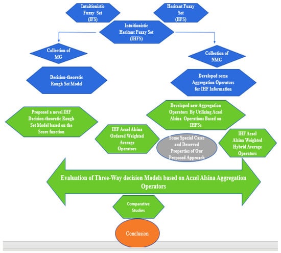
Figure 1.
Flow Chart of the proposed work.
- First, we presented novel aggregation operators and basic operational laws of IHFSs, exploring the fundamental notion of Aczel-Alsina and . Using Aczel-Alsina and , we developed a series of novel operators, such as operators, and verified their novelty with some properties.
- To test the feasibility and reliability of our proposed operators, we designed a few special cases, including -ordered weighted and -hybrid weighted () average operators with their fundamental properties.
- Additionally, we designed a novel three-way decision-theoretic rough set model in this article. This approach utilized new steps for 3WD, including the design of Aczel Alsina aggregation operators and the development of score function and accuracy function to classify participants.
- Using the proposed model, we provided a case study of business, where making the best decision for investment is a significant issue for investors. To address this issue, we developed a model consisting of different companies, and according to the Bayesian theory of risk, we discussed cost parameter tables from experts in detail under the variation of conditional probability.
- We discussed an influenced study to visualize the effectiveness of the parametric values of the conditional probabilities on the results of our presented model.
- Finally, we compared our developed approach with existing models of AOs to check its validity, authenticity, and effectiveness.
The rest of the paper is organized as follows: we quickly go over some of the core concepts of Aczel-Alsina and some generalizations of fuzzy sets and revisit the idea of DTRS in Section 2. In Section 3, we reorganize three-way decision rules based on DTRS using aggregation operators for IHFNs. In Section 4, we describe the series of novel Aczel-Alsina aggregation operation rules for the IHFNs, such as the IHF Aczel-Alsina weighted averaging operator, the IHF Aczel-Alsina order weighted averaging operator, and the IHF Aczel-Alsina hybrid averaging operator, and their useful features. In Section 5, we develop an algorithm for handling 3WD difficulties, where the characteristic values are represented as IHF data using the operator. In Section 6, an illustration of choosing a suitable company for investment evaluated by the suggested model is also given. We discuss how a parameter affects the classification order of options, and, to show the superiority and sensitivity of the developed approach, a comparative analysis is added in Section 7. Finally, Section 8 concludes the paper.
2. Preliminaries
In this section, we review several important theories of intuitionistic hesitant fuzzy sets and some concepts related to Aczel-Alsina , , and aggregation operators. The Table 1 is added to show the description of symbols used in the article.

Table 1.
List of abbreviations.
2.1. A Basic Review of Intuitionistic Hesitant Fuzzy Sets
Atanassov [9] proposed the theory of IFS as an extension of FS. While FS provides the degree of membership of an object in a specific set [0, 1], IFS provides both the degree of membership and the degree of non-membership simultaneously.
Definition 1 [9].
An IFS on is denoted via the two mappings and . Mathematically, it is shown by the following structure:
where and represents the MG and NMG including the condition , for each .
For every IFS in , we denote Then is called as the indeterminacy grade of to .
Tahir et al. [14] introduced a more generalized version of IFSs by combining them with HFS, known as IHFSs. In IHFSs, the MG and NMG represent the collection of elements from [0, 1]. The fundamental definition and operations are provided below.
Definition 2 [14].
An IHFS on is symbolized via the two mappings and . Mathematically, it is shown by the following structure:
where and are collection of several numbers from , indicating the possible MGs and NMGs of the object to the collection with the condition that , respectively.
For convenience, throughout the studies, is considered as IHFN.
Definition 3.
For any IHFNs , the score and accuracy functions are defined and denoted as
where, , .
Definition 4 [14].
Suppose = (, ), = (, ) are intuitionistic hesitant fuzzy sets (IHFSs), and a few fundamental operations are characterized as follows:
- (i)
- (ii)
- (iii)
- (iv)
- (v)
Definition 5.
Let be a group of IHFS and the weights for , and . Then, the IHFPWA operator is a function IHFPWA: where
where,
Definition 6.
For IHFSs , with their weights such that and . A function IHFPOWA: , is defined as
2.2. An Overview of Aczel-Alsina Operators
Triangular norms () are a particular class of functions that can be utilized to explain the intersection of fuzzy logic and FSs. Menger [22] first introduced the concept of which have been used in various decision-making and data-aggregation applications. In this section, we discuss the essential concepts that are vital for the development of this paper.
Definition 7.
A mapping : [0, 1]×[0, 1] → [0, 1] is a is satisfied following propertie ∈ [0, 1],
- (i)
- Symmetry: (, ) = (, ).
- (ii)
- Associativity: (, (, )) = ( (, ), ).
- (iii)
- Monotonicity: (, ) (, ) if
- (iv)
- One Identity: (1, ) = .
Examples of are → ∈ [0, 1],
- (i)
- Product triangular norm: (, ) = . ;
- (ii)
- Minimum triangular norm: (, ) = min (, ).
- (iii)
- Lukasiewicz triangular norm: (, ) = max ( + ).
- (iv)
- Drastic triangular norm:
Definition 8.
A mapping : [0, 1]×[0, 1] → [0, 1] is if the following axioms are satisfied: ∈ [0, 1],
- (i)
- Symmetry: (, m) = (, ).
- (ii)
- Associativity: (, (, )) = ( (, ), ).
- (iii)
- Monotonicity: (, ) (, ) if .
- (iv)
- Zero Identity: (0, ) = .
Examples of are → ∈ [0, 1]
- (i)
- Probabilistic sum triangular co norm: (, ) = +;
- (ii)
- Maximum triangular co norm: (, ) = max (, ).
- (iii)
- Lukasiewicz triangular co norm: (, ) = min { + }.
- (iv)
- Drastic triangular co norm:
Definition 9 [23].
Aczel-Alsina presented novel and which are represented as
and
2.3. Three-Way Decision Based on DTRS
DTRS is a well-known model for three-way decision-making based on Bayesian decision theory that minimizes the risk of multiple decisions [38]. The resulting approach is similar to hypothesis testing in statistics. In hypothesis testing, a hypothesis is accepted if there is sufficient evidence supporting it, rejected if there is sufficient evidence refuting it, and needs further evaluation if there is insufficient evidence supporting or refuting it. This interpretation justifies three-way decision-making based on the risk or cost of various decisions and requires an understanding of the cost of acquiring and applying evidence.
The 3WDM with DTRS theory [38] is succinctly explained here. It begins with a set of states designating, respectively, that components are in and not in . For both of these states, a series of actions is taken as , where and respectively, represent the classification of an object ’s acceptance , deferment , and rejection decision. The positive region , boundary region , and negative region ) are three disjoint regions. Moreover, as indicated in Table 2, a matrix provides the cost parameters. The costs associated with the actions and when an element goes to are , , and . However, the expenses for the corresponding three actions are denoted by , , and when an item does not belong to
Table 2.
Cost parameter matrix.
Since , by using the Bayesian risk decision theory [38], for the element , the classification losses associated with the three actions are expressed as follows:
For the minimum-loss decisions, the DTRS theory presents the following decision rules:
- (1)
- If and then .
- (2)
- If and , then .
- (3)
- If and then .
According to the Bayesian decision process [38], always choose the action plan with the lowest decision-making risk as the first choice.
3. A New DTRS Model Based on Intuitionistic Hesitant Fuzzy Sets
In this section, we will create a DTRS model for IHFSs based on 3WDs. First, we will construct a cost parameter matrix with the IHFNs presented in Table 3. As shown in Table 3, the values correspond to IHFNs . and represent the degrees of the loss of IHFNs due to taking action of , , and when the element belongs to the state . On the other hand, , , and represent the degrees of the loss caused when the element belongs to the state .
Table 3.
Intuitionistic hesitant risk information.
Given the prerequisites of
Based on (1)–(3), the expected losses under different actions can be denoted as follows:
According to the operations of IHFNs, the expected losses can be further presented as
The score functions for expected losses are designed for the above actions.
The accuracy functions for expected losses are designed for the above actions.
With the concept of score functions, we develop some novel decision rules.
- (1)
- If then .
- (2)
- If then .
- (3)
- If then
4. Aczel-Alsina Operators for Intuitionistic Hesitant Fuzzy Sets
The following section explains the Aczel-Alsina operations for IHFSs and investigates various fundamental characteristics of these functions. The triangular norm and triangular co-norm are characterized based on Aczel-Alsina, and the product and sum , are presented for IHFSs as shown below.
Definition 10.
Let be two intuitionistic hesitant fuzzy numbers and , with ≥ 1 and > 0. Here, we consider and as MG and NMG for IHFNs for Aczel-Alsina aggregation operators. Then, operations based on IHFNs are defined as
- (i)
- =
- (ii)
- (iii)
- (iv)
Theorem 1.
For two IHFNs , with ≥ 1, > 0. We have
- (i)
- (ii)
- (iii)
- (iv)
- (v)
Proof.
For the three IHFNs and and , as indicated in Definition 10, we have
- (i)
- (ii)
- It is straightforward.
- (iii)
- let then using this, we get
- (iv)
- (v)
- (vi)
- □
Intuitionistic Hesitant Fuzzy Aczel-Alsina Average Operators
Now, we will introduce some IHF average aggregation operators based on the Aczel-Alsina operations.
Definition 11.
For IHFNs , the weight for the with 0, and . Then operator is a function: : defined as
From Definition 11, we obtain the following theorem for IHFNs.
Theorem 2.
Suppose is an accumulation of IHFNs. The assigned weight for each . The obtained result of IHFNs applying operator is again IHFN:
Proof.
Through the applying of the mathematical induction technique, we are able to prove the Theorem in the following manner:
(I) Let , then
Based on the Definition 10, we obtain
Hence, Equation (5) is satisfied for .
(II) Consider Equation (5) is fulfilled for , then it is obtained
Now, for +1, we get
Thus Equation (5) is valid for .
(I), (II) implies that it can be deduced; Equation (5) is satisfied for any .
Using the IHF WA operator, we could successfully illustrate the related features. □
Property 1. (Idempotency).
If all are equal, that is, for all , then .
Property 2. (Boundedness).
If all be a set of IHFNs. Consider and . Then,
Property 3. (Monotonicity).
If all and being two sets of IHFNs. Let then .
Now, we produce IHF Aczel-Alsina ordered weighted averaging () operations.
Definition 12.
Suppose being an accumulation of IHFNs and the assigned weight for each with 0, and . Then operator is a function:→: defined as
where () are the permutation of , containing for all
From Definition 12, we obtain the result shown below.
Theorem 3.
Suppose being an accumulation of IHFNs. the weight for each ). The aggregated result of IHFNs by operator is also IHFN:
where ( ) are the permutation of every , containing for all
The associated attributes can successfully be confirmed by applying the operator.
Property 4. (Idempotency).
If all are equivalent, that is, for all , then .
Property 5. (Boundedness).
If all being a group of IHFNs. Let and . Then,
Property 6. (Monotonicity).
If all and are two sets of IHFNs. Let then .
Property 7. (Commutativity).
Let and be two sets of IHFNs, then where is any permutation of
Definition 11 and Definition 12 provide a direction for developing hybrid aggregation operators which are defined below.
Definition 13.
Suppose , being an accumulation of IHFNs. The assigned weight for each and a new Then operator is a function: : defined as
where () represents the permutation of all , containing for all
Definition 13 gives us the idea of following theorem.
Theorem 4.
For IHFNs . The result using operator for IHFNs is still an IHFN,
Proof.
The proof is omitted. □
Theorem 5.
The operators are a generalization of the and operators.
Proof.
(1) let Then
(2) let .
Then
which completes the proof. □
5. An Algorithm for Three-Way Decision Making under Intuitionistic Hesitant Fuzzy Environment
This section demonstrates the use of operators for three-way decision making through intuitionistic hesitant fuzzy data. We outline five steps for selecting 3WD rules for different participants. Let , , be the group of actions, and be the set of states. Let be the conditional probability vector, where . Figure 2 displays the established algorithm of the developed approach.

Figure 2.
Algorithm of Three-Way Decision.
Step 1. Evaluate the intuitionistic hesitant fuzzy matrix according to the actual condition,
Step 2. For alternatives , calculate all the IHF numbers into a general result utilizing operator in the following:
Step 3. Calculate the expected losses of for taking actions.
Step 4. Aggregate the score function varied according to total IHF information .
Step 5. According to the 3WD rules (4)–(6) to acquire the corresponding decisions.
Step 6. End
6. Numerical Example
An investigative example is provided in this part for making the best decision to invest in a company to minimize loss or risk and obtain maximum profit.
6.1. Explanation of the Problem
At the present time, businessmen face many problems, but one of the most significant and sensitive issues is where to invest to maximize benefits while minimizing risks. Several theories have been proposed [38,41] by researchers to address this question, including Bayesian risk theory [44]. In this section, we propose a model to help businessmen make investment decisions more easily. Our model is based on the DTRS approach, which divides the investment space into three regions: accepted, rejected, and boundary regions.
Let us consider the case of Mr. X, who plans to invest in a business and has identified four globally ranked companies to evaluate for investment opportunities. To make the best investment decision with low business risk, four experts have been hired to evaluate the risk of each company. The assigned weights allocated by the experts are . Suppose the conditional probabilities for all four companies are the same, i.e., . In this scenario, a decision result is required.
6.2. The Decision-Making Steps
Step 1: The risk of each company is evaluated by four experts based on their comprehensive situation, and the results are presented in Table 4, Table 5, Table 6 and Table 7.
Table 4.
The risk given by E1.
Table 5.
The risk given by E2.
Table 6.
The risk given by E3.
Table 7.
The risk given by E4.
Step 2: The operator is applied to integrate the evaluation information from individual decisionmakers into collective information .
Step 3: The expected losses are calculated by assuming constant probability for all the alternatives mentioned above, and the results are listed in Table 8.
Table 8.
Aggregation of risk values by operators.
Step 4. Aggregate the score numbers of each company, denoted as and the results are presented in Table 9.
Table 9.
Score results of expected losses.
Step 5. Based on the 3WD rules (4)–(6), the corresponding decision rule for each company can be determined. Currently, the investment judgment of each company largely depends on the expected value of its expected losses. The final decision result of each company is presented in Table 10.
Table 10.
Decision results.
Step 6. , , and are chosen as the suitable companies for investment for Mr. X.
7. The Effect of the Conditional Probabilities in this Method
Suppose the conditional probability values are changed from 0.30 to 0.70 in steps of 0.1, and the decision results based on rules (4)–(6) are listed in Table 11. To present the situation more intuitively where the 3WD results of each alternative change with the conditional probability, we show the results in Figure 3.
Table 11.
Effects of the probability values.
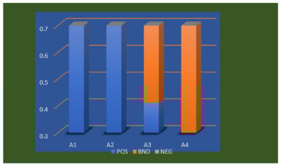
Figure 3.
Effects of conditional probability on the participants.
During the variation of the conditional probability values, some differences in results occur, but the changes seem to be very small. At a conditional probability of 0.3–0.5, alternatives – are classified as accepted, and is in the boundary region for investment, fortunately with no alternative in the rejected region. When the conditional probability is increased, a minor change is observed. At 0.6–0.7, and remain in the positive region for investors, and moves to the boundary region. Alternatives and are in the unclear environment.
Based on Figure 3, we can conclude that and are classified as accepted, while is in the unclear environment. The classification of depends on the value of the probability. It is a positive outcome that, in this scenario, there is no alternative in the rejected region. However, it is important to note that in other situations, the rejected region may not be empty.
Comparative Analysis
In this section, we applied several existing AOs to the information provided by the decisionmakers in Table 5, Table 6, Table 7 and Table 8 to evaluate the validity and feasibility of our proposed methodologies. We compared our approach with IFWA [19], IFWG [18], IvIFAAWA [31], IvIFAAWG [45], HFAAW [25], IFDWA [46], FDWG [46], IFRAAWA [24], IFRAAOW [24], IFRAAHA [24], IHFPWA [14], and IHFPG [14] methods. The results of existing AOs operators are shown in Table 12.
Table 12.
Comparison of proposed and existing techniques.
- The analysis of Table 12 suggests that our proposed approach is more general than existing models.
- Our proposed model also provides more flexible acceptance results compared to Mahmood’s IFPWA [14].
- Additionally, we observed that IFWA [19], IFWG [18], HFAAW [25], IFDWA [46], IFDWG [46], IFRAAWA [24], IFRAAOW [24], and IFRAAHA [24] effectively handle intuitionistic fuzzy and hesitant fuzzy data. However, there are certain situations where these approaches may not be suitable. This demonstrates the dependability and effectiveness of the proposed model for decisionmakers.
- Table 12 also highlights that Senapati et al. developed IvIFAAWA [31] and IvIFAAWG [45] operators for interval valued intuitionistic fuzzy information, but comparison studies have shown that these approaches are not effective for intuitionistic hesitant fuzzy data. Therefore, our proposed approach provides a solution to address more complex and vague situations.

Figure 4.
Comparison of results with existing approaches.
8. Conclusions
Our paper focuses on the three-way decision model, a powerful tool for decision making based on object attributes. This model has gained popularity due to its effectiveness in real-life situations such as the business, medical, and technology fields. However, decisionmakers often struggle with a lack of information and time. To address these challenges, we utilized intuitionistic hesitant fuzzy sets (IHFSs), which include membership-grade (MG) and non-membership grade (NMG) sets, and developed operators for three-way decision making.
One of the key contributions of our paper is the presentation of novel aggregation operators and basic operational laws of IHFSs. We explored the fundamental notion of Aczel-Alsina and and developed a series of novel operators, such as operators. We tested the feasibility and reliability of our proposed operators by designing special cases, such as -ordered weighted and -hybrid weighted () average operators with their fundamental properties. Furthermore, we developed a novel three-way decision-theoretic rough set model that utilized new steps for 3WD, such as designing Aczel-Alsina aggregation operators and developing score and accuracy functions to classify participants. We provided a case study in business to showcase the effectiveness of our proposed model in addressing investment decision making. We constructed a model consisting of different companies and used the Bayesian theory of risk to discuss the cost parameter tables from experts in detail under the variation of conditional probability. We also discussed an influenced study to visualize the effectiveness of the parametric values of the conditional probabilities on the results of our presented model.
We compared our developed approach with existing AO models to demonstrate its validity, authenticity, and effectiveness. Our operators and techniques have practical applications in various fields, including networking analysis, risk assessment, and cognitive science, in uncertain situations. We will further investigate our novel techniques in the scope of multi-criteria development in the fuzzy environment and examine the idea behind our suggested methods within the perspective of square root fuzzy information [47,48]. Additionally, we will examine our ongoing research using a temporal intuitionistic fuzzy system [49,50].
Author Contributions
Conceptualization, W.A., T.S., H.G.T., F.A., M.Z.U., M.M.H.; methodology, W.A., T.S.; software, W.A.; validation, W.A., T.S., H.G.T., F.A., M.Z.U., M.M.H.; formal analysis, W.A., T.S.; investigation, W.A., T.S., H.G.T., F.A., M.Z.U., M.M.H.; resources, M.Z.U., M.M.H.; data curation, W.A., T.S., H.G.T.; writing—original draft preparation, W.A., T.S., H.G.T., F.A., M.Z.U., M.M.H.; writing—review and editing, M.Z.U., M.M.H.; visualization, W.A.; funding acquisition, M.M.H.; All authors have read and agreed to the published version of the manuscript.
Funding
The authors are grateful to King Saud University, Riyadh, Saudi Arabia, for funding this work through Researchers Supporting Project Number—RSP2023R18.
Institutional Review Board Statement
Not applicable.
Informed Consent Statement
Not applicable.
Data Availability Statement
Not applicable.
Conflicts of Interest
The authors declare no conflict of interest.
References
- Bourahla, M. Using Rough Set Theory for Reasoning on Vague Ontologies. Int. J. Intell. Syst. Appl. 2022, 14, 21–36. [Google Scholar] [CrossRef]
- Ardil, C. Vague Multiple Criteria Decision Making Analysis Method for Fighter Aircraft Selection. Int. J. Aerosp. Mech. Eng. 2022, 16, 133–142. [Google Scholar]
- Zadeh, L.A. Fuzzy sets. Inf. Control 1965, 8, 338–353. [Google Scholar] [CrossRef]
- Zhang, L.; Zhang, B. The quotient space theory of problem solving. Fundam. Inform. 2004, 59, 287–298. [Google Scholar]
- Pawlak, Z. Rough set theory and its applications to data analysis. Cybern. Syst. 1998, 29, 661–688. [Google Scholar] [CrossRef]
- Saraji, M.K.; Mardani, A.; Köppen, M.; Mishra, A.R.; Rani, P. An extended hesitant fuzzy set using SWARA-MULTIMOORA approach to adapt online education for the control of the pandemic spread of COVID-19 in higher education institutions. Artif. Intell. Rev. 2021, 55, 181–206. [Google Scholar] [CrossRef]
- Xie, X.; Jia, Z.; Shi, H.; Zhu, X. A Location–Time-Aware Factorization Machine Based on Fuzzy Set Theory for Game Perception. Appl. Sci. 2022, 12, 12819. [Google Scholar] [CrossRef]
- Kim, K.B.; Park, H.J.; Song, D.H. Combining Supervised and Unsupervised Fuzzy Learning Algorithms for Robust Diabetes Diagnosis. Appl. Sci. 2022, 13, 351. [Google Scholar] [CrossRef]
- Atanassov, K.T. On Intuitionistic Fuzzy Sets Theory; Springer: Berlin/Heidelberg, Germany, 2012; Volume 283. [Google Scholar]
- Torra, V. Hesitant fuzzy sets. Int. J. Intell. Syst. 2010, 25, 529–539. [Google Scholar] [CrossRef]
- Garg, H.; Keikha, A. Various aggregation operators of the generalized hesitant fuzzy numbers based on Archimedean t-norm and t-conorm functions. Soft Comput. 2022, 26, 13263–13276. [Google Scholar] [CrossRef]
- Sarkar, A.; Animesh, B. Dual hesitant q-rung orthopair fuzzy Dombi t-conorm and t-norm based Bonferroni mean operators for solving multicriteria group decision making problems. Int. J. Intell. Syst. 2021, 36, 3293–3333. [Google Scholar] [CrossRef]
- Pu, D.; Yu, M.; Yuan, G. Multiattribute Decision-Making Method Based on Hesitant Triangular Fuzzy Power Average Operator. Adv. Fuzzy Syst. 2022, 2022, 4467548. [Google Scholar] [CrossRef]
- Mahmood, T.; Ali, W.; Ali, Z.; Chinram, R. Power aggregation operators and similarity measures based on improved intuitionistic hesitant fuzzy sets and their applications to multiple attribute decision making. Comput. Model. Eng. Sci. 2021, 126, 1165–1187. [Google Scholar] [CrossRef]
- Yager, R.R. Generalized OWA aggregation operators. Fuzzy Optim. Decis. Mak. 2004, 3, 93–107. [Google Scholar] [CrossRef]
- Yager, R.R. Prioritized aggregation operators. Int. J. Approx. Reason. 2008, 48, 263–274. [Google Scholar] [CrossRef]
- Zhang, H.; Wei, G.; Chen, X. Spherical fuzzy Dombi power Heronian mean aggregation operators for multiple attribute group decision-making. Comput. Appl. Math. 2022, 41, 98. [Google Scholar] [CrossRef]
- Xu, Z.; Yager, R.R. Some geometric aggregation operators based on intuitionistic fuzzy sets. Int. J. Gen. Syst. 2006, 35, 417–433. [Google Scholar] [CrossRef]
- Xu, Z. Intuitionistic fuzzy aggregation operators. IEEE Trans. Fuzzy Syst. 2007, 15, 1179–1187. [Google Scholar] [CrossRef]
- Ayub, N.; Aslam, M. Dual Hesitant Fuzzy Bonferroni Means and Its Applications in Decision-Making. Ital. J. Pure Appl. Math. 2022, 48, 32–53. [Google Scholar]
- Hadi, A.; Khan, W.; Khan, A. A novel approach to MADM problems using Fermatean fuzzy Hamacher aggregation operators. Int. J. Intell. Syst. 2021, 36, 3464–3499. [Google Scholar] [CrossRef]
- Menger, K. Statistical metrics. Proc. Natl. Acad. Sci. USA 1942, 28, 535. [Google Scholar] [CrossRef] [PubMed]
- Aczél, J.; Alsina, C. Characterizations of some classes of quasilinear functions with applications to triangular norms and to synthesizing judgements. Aequ. Math. 1982, 25, 313–315. [Google Scholar] [CrossRef]
- Ahmmad, J.; Mahmood, T.; Mehmood, N.; Urawong, K.; Chinram, R. Intuitionistic Fuzzy Rough Aczel-Alsina Average Aggregation Operators and Their Applications in Medical Diagnoses. Symmetry 2022, 14, 2537. [Google Scholar] [CrossRef]
- Senapati, T.; Chen, G.; Mesiar, R.; Yager, R.R.; Saha, A. Novel Aczel–Alsina operations-based hesitant fuzzy aggregation operators and their applications in cyclone disaster assessment. Int. J. Gen. Syst. 2022, 51, 511–546. [Google Scholar] [CrossRef]
- Ashraf, S.; Ahmad, S.; Naeem, M.; Riaz, M.; Alam, A. Novel edas methodology based on single-valued neutrosophic aczel-alsina aggregation information and their application in complex decision-making. Complexity 2022, 2022, 2394472. [Google Scholar] [CrossRef]
- Wang, H.; Xu, T.; Feng, L.; Mahmood, T.; Ullah, K. Aczel–Alsina Hamy Mean Aggregation Operators in T-Spherical Fuzzy Multi-Criteria Decision-Making. Axioms 2023, 12, 224. [Google Scholar] [CrossRef]
- Sarfraz, M.; Ullah, K.; Akram, M.; Pamucar, D.; Božanić, D. Prioritized Aggregation Operators for Intuitionistic Fuzzy Information Based on Aczel–Alsina T-Norm and T-Conorm and Their Applications in Group Decision-Making. Symmetry 2022, 14, 2655. [Google Scholar] [CrossRef]
- Jin, H.; Hussain, A.; Ullah, K.; Javed, A. Novel Complex Pythagorean Fuzzy Sets under Aczel–Alsina Operators and Their Application in Multi-Attribute Decision Making. Symmetry 2022, 15, 68. [Google Scholar] [CrossRef]
- Senapati, T.; Chen, G.; Yager, R.R. Aczel–Alsina aggregation operators and their application to intuitionistic fuzzy multiple attribute decision making. Int. J. Intell. Syst. 2021, 37, 1529–1551. [Google Scholar] [CrossRef]
- Senapati, T.; Chen, G.; Mesiar, R.; Yager, R.R. Novel Aczel–Alsina operations-based interval-valued intuitionistic fuzzy aggregation operators and their applications in multiple attribute decision-making process. Int. J. Intell. Syst. 2022, 37, 5059–5081. [Google Scholar] [CrossRef]
- Yao, Y. Three-way decisions and cognitive computing. Cogn. Comput. 2016, 8, 543–554. [Google Scholar] [CrossRef]
- Yao, Y. An outline of a theory of three-way decisions. In International Conference on Rough Sets and Current Trends in Computing; Springer: Berlin/Heidelberg, Germany, 2012. [Google Scholar]
- Yao, Y. The geometry of three-way decision. Appl. Intell. 2021, 51, 6298–6325. [Google Scholar] [CrossRef]
- Mehmood, A.; Shaikh, I.U.H.; Ali, A. Application of Deep Reinforcement Learning for Tracking Control of 3WD Omnidirectional Mobile Robot. Inf. Technol. Control 2021, 50, 507–521. [Google Scholar] [CrossRef]
- Zhang, C.; Ding, J.; Li, D.; Zhan, J. A novel multi-granularity three-way decision making approach in q-rung orthopair fuzzy information systems. Int. J. Approx. Reason. 2021, 138, 161–187. [Google Scholar] [CrossRef]
- Yao, Y.; Deng, X. Sequential three-way decisions with probabilistic rough sets. In Proceedings of the IEEE 10th International Conference on Cognitive Informatics and Cognitive Computing (ICCI-CC’11), Banff, AB, Canada, 18–20 August 2011. [Google Scholar]
- Liu, D.; Yao, Y.; Li, T. Three-way investment decisions with decision-theoretic rough sets. Int. J. Comput. Intell. Syst. 2011, 4, 66–74. [Google Scholar]
- Zhang, K.; Dai, J. A novel TOPSIS method with decision-theoretic rough fuzzy sets. Inf. Sci. 2022, 608, 1221–1244. [Google Scholar] [CrossRef]
- Qian, Y.; Hu, Z.; Sang, Y.; Liang, J. Multigranulation decision-theoretic rough sets. Int. J. Approx. Reason. 2014, 55, 225–237. [Google Scholar] [CrossRef]
- Liang, D.; Liu, D. Deriving three-way decisions from intuitionistic fuzzy decision-theoretic rough sets. Inf. Sci. 2015, 300, 28–48. [Google Scholar] [CrossRef]
- Ali, Z.; Mahmood, T.; Smarandache, F. Three-Way Decisions with Single-Valued Neutrosophic Uncertain Linguistic Decision-Theoretic Rough Sets Based on Generalized Maclaurin Symmetric Mean Operators. In Neutrosophic Operational Research; Springer: Berlin/Heidelberg, Germany, 2021; pp. 71–101. [Google Scholar] [CrossRef]
- Wagh, M.; Nanda, P.K. Decision-Theoretic Rough Sets based automated scheme for object and background classification in unevenly illuminated images. Appl. Soft Comput. 2022, 119, 108596. [Google Scholar] [CrossRef]
- Zhao, X.R.; Hu, B.Q. Three-way decisions with decision-theoretic rough sets in multiset-valued information tables. Inf. Sci. 2018, 507, 684–699. [Google Scholar] [CrossRef]
- Senapati, T.; Mesiar, R.; Simic, V.; Iampan, A.; Chinram, R.; Ali, R. Analysis of interval-valued intuitionistic fuzzy aczel–alsina geometric aggregation operators and their application to multiple attribute decision-making. Axioms 2022, 11, 258. [Google Scholar] [CrossRef]
- Seikh, M.R.; Mandal, U. Intuitionistic fuzzy Dombi aggregation operators and their application to multiple attribute decision-making. Granul. Comput. 2019, 6, 473–488. [Google Scholar] [CrossRef]
- Ul Haq, I.; Shaheen, T.; Ali, W.; Senapati, T. A Novel SIR Approach to Closeness Coefficient-Based MAGDM Problems Using Pythagorean Fuzzy Aczel–Alsina Aggregation Operators for Investment Policy. Discret. Dyn. Nat. Soc. 2022, 2022, 5172679. [Google Scholar] [CrossRef]
- Radenovic, S.; Ali, W.; Shaheen, T.; ul Haq, I.; Akram, F.; Toor, H. Multiple Attribute Decision-Making Based on Bonferroni Mean Operators under Square Root Fuzzy Set Environment. J. Comput. Cogn. Eng. 2022. [Google Scholar] [CrossRef]
- Talari, P.; Suresh, A.; Kavitha, M.G. An Intelligent Medical Expert System Using Temporal Fuzzy Rules and Neural Classifier. Intell. Autom. Soft Comput. 2023, 35, 1053–1067. [Google Scholar] [CrossRef]
- Ali, W.; Shaheen, T.; Haq, I.U.; Toor, H.G.; Akram, F.; Jafari, S.; Uddin, M.Z.; Hassan, M.M. Multiple-Attribute Decision Making Based on Intuitionistic Hesitant Fuzzy Connection Set Environment. Symmetry 2023, 15, 778. [Google Scholar] [CrossRef]
Disclaimer/Publisher’s Note: The statements, opinions and data contained in all publications are solely those of the individual author(s) and contributor(s) and not of MDPI and/or the editor(s). MDPI and/or the editor(s) disclaim responsibility for any injury to people or property resulting from any ideas, methods, instructions or products referred to in the content. |
© 2023 by the authors. Licensee MDPI, Basel, Switzerland. This article is an open access article distributed under the terms and conditions of the Creative Commons Attribution (CC BY) license (https://creativecommons.org/licenses/by/4.0/).