Abstract
A pre-existing and inherited geostructural setting plays a fundamental role in preparing and developing large-scale slope deformational processes. These structures affect the kinematics of the process, the geometrical characteristics, and the geomorphological evolution. In the Apennine Belt, several deep-seated gravitational slope deformations (DSGSDs) that have evolved under a clear structural control have been recognized during the last decades, but none with a continuous and well-defined basal shear zone (BSZ). The structurally-controlled DSGSD of Luco dei Marsi represents the first case of a DSGSD in the Apennine Belt with a well-defined BSZ. Starting from a detailed study of the process and the reconstruction of a morpho-evolutionary model of the slope, a series of numerical modelings were performed for the study of the DSGSD. The analyses allowed us to reconstruct: (i) the mechanism of the process, (ii) the rheological behavior of the rock mass, and (iii) the main predisposing factors of the gravitational deformation. Numerical modeling has demonstrated the significant role played by the inherited structures on the DSGSD and, in particular, the importance of an intensely jointed stratigraphic level in the development of the BSZ.
1. Introduction
The onset and evolution of deep-seated gravitational slope deformations (DSGSDs) are controlled by two main factors [1,2,3,4]: (i) inherited and pre-existing geostructural elements (e.g., anisotropies, morpho-structural conditions, tectonic elements, weak planes or zones, karst); (ii) variations in stress-strain conditions (e.g., debuttressing, erosional processes, change in water table, tectonic stresses). The first group influences all the geological evolution of the slope on long-term time span, while the second group induces significant variation in the stress regime over short- and mid-term time spans [5,6,7,8,9]. In particular, the structural setting of mountain slopes influences the shape and dimension of rock slope deformations as their kinematic is often controlled by pre-existing discontinuities or weak zones, which act as preferential sliding surfaces, basal shear zone, or lateral releases.
Among the inherited and pre-existing factors, tectonic structures such as folds and faults are certainly the most important elements [1,10,11,12,13,14,15], in addition to bedding planes or schistosity [16,17,18]. Locally, DSGSDs are strictly related to karst phenomena [19,20] and dissolution of evaporitic rocks [21]. The evidence that inherited tectonic structures played a fundamental role in driving geometry and kinematic of DSGSDs has been acknowledged by several authors also in the central Apennine Belt [15,16,20,21,22,23,24,25].
DSGSDs are usually featured by mass rock creep (MRC) processes [26,27,28] and ductile and visco-plastic deformations along shear planes and sliding surfaces [1]. In detail, MRC is driven by the rock mass viscosity, the structural setting of the slopes, the jointing state of rock masses, and the weathering of igneous and metamorphic rocks [4,10,12]. Geomechanical conditions and inherited structures can greatly influence the rheological properties of the deformed rock masses and the MRC processes [17].
Nowadays, the role of geostructural elements in slope dynamics is thoughtfully investigated through numerical models. These analyses of DSGSDs were carried out since the 1970s [29]. In more recent years, the growth of new technologies contributes to the increase in the number of numerical modelings on these phenomena [2,12,14,16,19,20,23,30,31,32,33,34,35]. In the last years, some numerical analyses were performed also on large-scale gravitational deformation on the planet Mars [36,37].
The study area lies in central Italy, within the axial zone of the Apennine Belt and along the western edge of the Fucino Basin, a Quaternary, wide continental depression (Figure 1). Several DSGSDs have been detected and analyzed in the last two decades in the central Apennines, both for scientific purposes and related hazard and risk. Regarding the latter, it is worth underlining how these gravity-induced deformations can evolve as catastrophic rock slope failures, e.g., [25], or be accompanied by secondary landslides threatening infrastructures, roads, villages, and elements of cultural heritage, as it happens [38] in the study area (see insert in Figure 1).
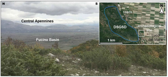
Figure 1.
Panoramic view of the Fucino Basin, taken from the Luco dei Marsi ridge (from SW). The insert contains a panoramic view (produced with Google Earth) of the DSGSD, and the main anthropic elements present in the study area.
The Meso-Cenozoic carbonate sequence outcropping near the village of Luco dei Marsi is affected by an evident DSGSD [39]. The process is revealed by several morphological features, such as grabens, trenches, downhill- and uphill-facing scarps, bulging, and landslides, variously distributed along the slope. The Luco dei Marsi DSGSD shows the first evidence of a clear and well-extended Basal Shear Zone (BSZ) in the central Apennines. This driven element is localized within Middle-Upper Cretaceous, Rudist-bearing massive limestones which underlies a—some meters thick—highly-jointed level (hereafter, HJL) developed into thinly-layered, biodetritic limestones featuring the lowermost part of the Upper Cretaceous sequence in the Luco dei Marsi ridge.
In this study, sequential numerical modeling was performed to define the main characteristics of the DSGSD evolution. The modeling has been based on the morpho-evolutionary model of the slope, reconstructed since early Pleistocene onward through geological and geomorphological evidence, and on the geomechanical characteristics of the rock masses determined through field measurements and laboratory tests. Due to the scale of the analyzed process, the behavior of jointed rocks was simulated through an equivalent continuum approach, considering the presence of joint sets and the time-dependent deformations of the HJL. The numerical models allowed us to define the kinematics of the process, the rheological behavior of the rock masses, and the main controlling factors for the DSGSD.
2. Geological Setting
The Luco dei Marsi carbonate ridge extends in an NNW-SSE direction and borders the western side of the Fucino Basin (Figure 1), the main Quaternary continental basin of the central Apennine Belt, e.g., [40,41]. The geological structure corresponds to a wide, symmetric anticline (Figure 2), which originated during the Late Miocene orogenesis by folding a sedimentary multilayer made by Lower to Upper Cretaceous, shallow-water carbonates, and Middle Miocene carbonate ramp deposits. These last ones are scattered in a few outcrops along the eastern edge of the slope, where they unconformably overlie the Upper Cretaceous sequence.
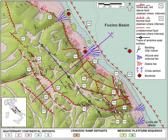
Figure 2.
Geological map of the Luco dei Marsi area, modified after Di Luzio et al. [39]. Legend: Quaternary deposits: (1) landslides; (2) residual clay deposits; (3) talus slope deposits; (4) eluvial-colluvial deposits; (5) alluvial and lacustrine deposits of the Fucino Basin; (6) middle Miocene (mM) ramp deposits (Calcari a Briozoi and Lithotamni Auctt.); (7) Upper Cretaceous limestones; (8) middle-Upper Cretaceous limestones including both the BSZ (basal shear zone) and the HJL (highly-jointed level). T1–T5 and F1–F7 indicate the number of strike-slip and normal faults, as reported in the multiple-step, conceptual model. Borehole B1–B3 data were taken from https://www.isprambiente.gov.it (accessed on 21 January 2021).
The anticline setting is characterized by parallel layering with a constant thickness and a cylindrical geometry. This folding style is typical of most of the fault-bend folds developed into the thick carbonate sequences of the central Apennines, which are composed of homogeneous material. The fold is affected by syn- and post-orogenic brittle deformation. The HJL was observed within the lowermost section of the Upper Cretaceous sequence (Cenomanian in age). This level, found right above the BSZ, is characterized by closely-spaced, open fractures mainly perpendicular to bedding planes and parallel to the fold axial surface (Figure 3a). These features can be interpreted as longitudinal joints developed in the fold extrados, near the hinge zone, as a response to tensile strain in thinly-layered beds.
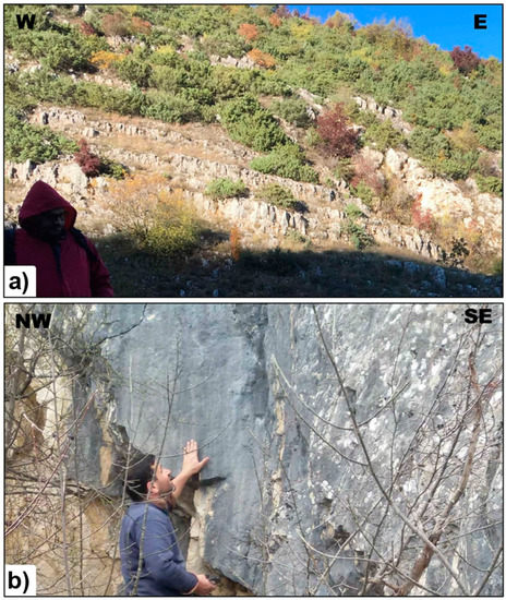
Figure 3.
Stratigraphic sequence and main tectonic elements: (a) Upper Cretaceous, thinly-layered, biodetritic limestones in the southern sector of the ridge affected by severe jointing; (b) left hand resting on a normal fault plane along the eastern edge of the Luco dei Marsi slope (F1 in Figure 2).
NNW-SSE-oriented normal faults dissect the entire anticline, whereas later WNW-ESE trending strike-slip faults—mainly with left-lateral kinematics—are concentrated in the southern sectors. The first system marks the eastern boundary of the carbonate ridge and is composed of several faults (F1–F4 in Figure 2 and F1 in Figure 3b) disposed in a cascade-like structure; the vertical down-throw is limited to a few tens of meters along each fault, but the whole system accommodates a cumulative displacement of more than 100 m.
A multiple-step model of the slope’s morphotectonic evolution was drawn in Di Luzio et al. [39], which included the main erosive, depositional, and tectonic events since the Early Pleistocene to the historical times (Figure 4). According to the model, apex of normal faulting, linked to the opening of the Fucino Basin, occurred in the Late Pleistocene. Such a tectonic process determined the slope lateral unconfinement necessary to trigger the DSGSD. Nowadays, the fault activity is shifted basin-ward along the Luco dei Marsi structural line (LMF, F0 in Figure 2).
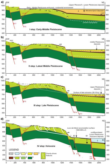
Figure 4.
Multiple-step, conceptual model of the Quaternary morphotectonic evolution of the Luco dei Marsi ridge and the Fucino Basin western edge, modified after Di Luzio et al. [39]. (a) subaerial erosion following deposition of Upper Pliocene-Lower Pleistocene alluvial and lacustrine deposits; (b) renewed erosion after sedimentation of Middle Pleistocene lacustrine, fluvial, and deltaic deposits; (c) late Pleistocene lacustrine environment (the intense tectonic activity along the edge of the slope activated the DSGSD process); (d) basin-ward migration of tectonic activity along the LMF, full development of the DSGSD. Legend: (1) talus deposits; (2) undifferentiated Quaternary deposits of the Fucino Basin; (3–5) Upper, Middle, and Lower Pleistocene alluvial and lacustrine deposits; (6) Miocene flysch deposits; (7) layered, Upper Cretaceous limestones, upper section; (8) lower section including the HJL and Middle-Upper Cretaceous massive limestones hosting the BSZ; (9) Lower Cretaceous limestone.
3. DSGSD and BSZ
Evidence of the Luco dei Marsi DSGSD are different kinds of geomorphic features distributed over an area of about 4 km2, with a NNW-SSE-oriented elongation axis (Figure 5). Trenches, plurimetric in length and width, are distributed both along the slope edge (Figure 6a) and the internal sectors, where they are often associated with grabens or downhill- and uphill-facing scarps (Figure 6b,c). In the same areas, roughly corresponding to the fold axial zone, complex features such as grabens and ridge-top depressions were also observed, as well as bulging and landslides at the toe of the carbonate slope [38]. The activity of the DSGSD during the last 30 years, of the order of a few mm/yr, was acknowledged by means of analysis of DInSAR data and time-series elaboration [39].
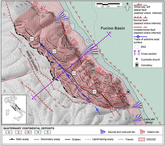
Figure 5.
Inventory map of geomorphological features ascribable to the Luco dei Marsi DSGSD and location of the BSZ outcrops along the southern edge, modified after Di Luzio et al. [39]. Structural and tectonic elements from Figure 2 are reported. Quaternary deposits: (1) landslides; (2) residual clay deposits; (3) talus slope deposits; (4) eluvial-colluvial deposits; (5) alluvial and lacustrine deposits of the Fucino Basin. G1–G4 = gravitational grabens.
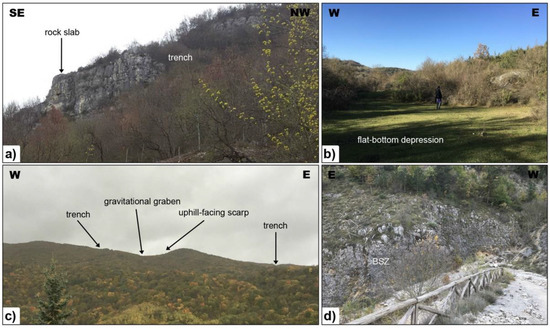
Figure 6.
Morphological features of the Luco dei Marsi DSGSD: (a) trench; (b) gravitational graben with flat-bottom depression; (c) system of trench, gravitational graben, and uphill-facing scarp; (d) outcrop of the BSZ.
As a singular feature in the geological framework of the central Apennines, a basal shear zone (BSZ) was observed along a deep valley incision in the southern, lower sector of the slope (Figure 5). With a maximum observable thickness of about 5 m and a low dip angle towards the Fucino Basin (Figure 6d), the BSZ is made by a cataclastic rock mass composed of intensely-jointed, centimetric blocks (GSI = 20) with calcite-filled veins and a fine matrix. A tectonic origin of the cataclastic zones has been discarded since (i) the anticline is a wide structure formed in the hanging-wall of a buried main thrust without secondary features such as splays, back-thrusts, or out-of-sequence features; (ii) the gently dipping attitudes of the BSZ deny a link with the high-angle longitudinal normal faults or the transverse transtensional faults; (iii) no evidence of low-angle normal faults was observed at the meso-ac macro-scale.
4. Engineering-Geological Model
To perform the numerical modelings, a detailed engineering-geological model of the ridge affected by the DSGSD was designed. The model was based on the stratigraphic and structural setting of the slope, the geological evolution of the area, and the physical-mechanical characteristics of rock masses deriving from site surveys and laboratory tests. The data on the slope setting and its Quaternary evolution are directly from the studies previously performed on the DSGSD [39]; the geomechanical data, instead, are described below. Finally, laboratory data on rock samples derive from specifically performed laboratory tests [42].
4.1. Rock Matrix Characteristics
The definition of the physical and mechanical properties of the rock matrix was based on laboratory tests. These tests were carried out on n.4 rock samples taken in the southern sector of the DSGSD. Among these, n.2 samples (C_1 and C_2) were taken inside the Upper Cretaceous sequence, and n.2 samples (C_3 and C_4) were collected within the BSZ. Physical analyses and UCS tests were carried out on each specimen (Table 1), even if the determination of the elastic parameters was possible only for the two samples of the deformed mass. A synthesis of the laboratory data used for the characterization is reported in Martino et al. [42].
For the two BSZ specimens, in the absence of data on the elastic parameters, the evaluation of the Young modulus and the Poisson ratio was carried out on the basis of the other samples. The elastic modulus was determined through the average ratio of the UCS strength of intact limestone (C_1 and C_2), by applying the same ratio to the BSZ specimens. The Poisson ratio was instead considered equal to the average value of intact limestone. The viscosity of the involved rock mass, not directly analyzed through laboratory tests, was based on the literature dealing with limestones similar to the ones involved in the here considered case study [17,18,19,20]. The viscosity of the HJL at the base of Upper Cretaceous limestones was derived from sensitivity analyses conducted through the numerical model. The main physical and mechanical properties of rock matrix constituting the mass affected by the slope deformation are summarized in Table 2.

Table 1.
Synthesis of physical and mechanical parameters derived from the laboratory tests.
Table 1.
Synthesis of physical and mechanical parameters derived from the laboratory tests.
| Specimen | Lithology | Unit Weight | UCS Strength | Young Modulus | Poisson Ratio |
|---|---|---|---|---|---|
| - | - | γ | σc | E | υ |
| - | - | kN/m3 | MPa | MPa | - |
| C_1 | Intact limestone | 26.1 | 71.88 | 47,736 | 0.20 |
| C_2 | Intact limestone | 26.3 | 92.83 | 72,356 | 0.28 |
| C_3 | Limestone with calcite veins | 25.6 | 40.56 | 29,088 | 0.24 |
| C_4 | Limestone with calcite veins | 26.4 | 9.30 | 6670 | 0.24 |
Table 2.
Synthesis of physical and mechanical parameters of the intact rock constituting the mass affected by the Luco dei Marsi DSGSD.
Table 2.
Synthesis of physical and mechanical parameters of the intact rock constituting the mass affected by the Luco dei Marsi DSGSD.
| Lithology | Unit Weight | UCS Strength | Young Modulus | Poisson Ratio | UCS/E Ratio | Viscosity |
|---|---|---|---|---|---|---|
| - | γ | σc | E | υ | σc/E | μ |
| - | kN/m3 | MPa | MPa | - | - | Pa·s |
| Intact limestone | 26.2 | 82.36 | 60,046 | 0.24 | 0.001394 | 2.00 × 10¹⁹ |
| Limestone with calcite veins | 26.0 | 24.93 | 17,879 | 0.24 | 0.001394 | 2.00 × 10¹⁷ |
4.2. Rock Mass Rheological Behavior
Starting from the characteristics of the intact rock and considering the jointing conditions as they have been surveyed, the properties of the rock mass were determined by exploiting the main correlations present in literature studies. In addition to the physical characteristics, the main parameters concerning a visco-plastic behavior were determined. The entire rock mass was previously portioned into several zones characterized by homogeneous properties. Regarding the structural setting of the slope, a cataclastic zone with extension as observed in the field was considered for each longitudinal normal fault reported in the cross-section.
The rock mass was characterized through an equivalent continuum approach, as previously carried out by several authors e.g., [17,23,43]. Such an approach transposes the rock mass in a continuous equivalent medium, endowed with a single constitutive law deriving from the characteristic of all the elements that characterize it [43,44,45,46,47]. The equivalent continuum approach is applicable to slope of considerable dimensions and is therefore widely used for the study of DSGSDs [2,12,14,16,19,20,23,31].
The unit weight was determined through the equations provided by Discenza et al. [48], considering the intact rock properties and the rock mass structure. The unit weight γm of jointed rocks was calculated through the following equation:
where γr is the unit weight of the intact rock, γj is the unit weight of the joint filling material in a particular joint set, aj is the average opening of the joints belonging to a particular set, lm is the average length of the considered mass, lj is the average length of a certain joint set, sj is the average spacing values of the discontinuities, Vt is the total volume of the considered mass, and ‘n’ is the number of joint sets.
For the fault zones corresponding to cataclastic rocks, the physical properties were attributed by considering a chaotic rock mass composed of rock blocks and a fine matrix. In this case, the unit weight γm of fault zones was calculated through the following relation:
where γc is the unit weight of different lithotypes, Vc is the volumetric ratio of each material, and ‘n’ is the number of discrete materials constituting the mass.
The rock mass strength was defined following the 2002 version Hoek–Brown failure criterion [45]. This approach allows the determination of the mechanical properties of a jointed rock mass considering the strength of rock matrix and the jointing conditions, as a function of the stress field existing within the slope. In this version, the criterion is expressed by the following equation:
In which σ1 and σ3 are the principal failure stress, σc is the uniaxial compressive strength, and mb, s, and a are empirical nondimensional constant related to the geological-structural setting of the rock mass. Specifically, mb can be determined through the intact rock constant mi, the degree of disturbance suffered by the rock after an excavation D, and the Geological Strength Index GSI, a parameter indicative of the jointing state of the mass and the characteristics of the discontinuities [49].
The tensile strength of rock mass was determined by using the alternative relationship of Hoek–Martin [50]. In this case, starting from the uniaxial compressive strength of intact rock σci, the tensile strength of the material T can be calculated through the following equation:
The elastic modulus of rock mass was estimated through the approach proposed by Sitharam et al. [43], which considers not only many geomechanical parameters but also the stress field acting on the rock. This approach is based on the determination of the Jf parameter, the Joint Factor [50,51,52], which directly depends on the jointing condition of the rock mass and on the geometrical and mechanical characteristics of discontinuities. The parameter Jf is given by the relation:
where Jv is the number of discontinuities per cubic meter of rock, n is a parameter related to the dip of the most frequent joint set, and r is an additional variable coefficient function of the uniaxial compressive strength of the intact rock [43,44,45,46,47,48,49,50,51,52,53]. The uniaxial compressive strength of the jointed rock σcj can be computed by the equation:
in which σci is the uniaxial compressive strength of the intact rock. Once these parameters have been determined, the Young modulus of jointer rock at null confinement Ej0 can be calculated through the procedure of Ramamurthy [51], expressed by the following relation:
where Ei0 is the Young modulus of intact rock at null confinement. Finally, the Young modulus of jointed rock mass Ej at any pressure of confinement σ3 can be determined as
Starting from the Young modulus of jointed rock and Poisson ratio, the other elastic parameters were determined according to the classical equation of the elasticity theory. The Bulk modulus K was calculated through the following equation:
while the shear modulus G was determined as
The viscosity of rock mass was determined by applying the equation of Discenza et al. [17], which allows us to estimate the rheological parameters of a jointed mass considering the viscosity of the matrix and the characteristics of discontinuities. With this approach, the viscosity of the rock mass μm was estimated through the following equation:
where μr is the viscosity of the stationary creep for intact rock, sj is the joint spacing (in cm), and dj is the joint dip (in degree). The proposed relation is reliable for a joint dip ranging from 0° up to 60° and for spacing values ranging from 0.01 m up to 1.50 m.
4.3. Rock Mass Joint Mechanical Behavior
The plastic behavior of main discontinuities sets was considered in the structural-dependent model. The characteristics of joint sets were determined through the Barton–Bandis strength model [54]:
where σn is the stress normal to the joint wall, φr is the residual friction angle of the failure surface, JRC is the joint roughness coefficient, and JCS is the joint wall compressive strength. In the Barton–Bandis model, the residual friction angle can be estimated through the following equation:
in which φb is the basic friction angle, r is the Schmidt rebound number on wet and weathered joint surfaces, and R is the Schmidt rebound number on dry and unweathered joint surface.
5. Numerical Modeling
Based on the engineering-geological model and the reconstructed geological evolution of the slope [39], a series of numerical models were implemented along the analyzed cross-section. The modeling was performed through the finite element software RS2 (v.11.015) by Rocscience [55]. The numerical domain was discretized into 102 regions, with 6 nodes triangular meshes. The plain-strain model was fully constrained at the bottom and x-constrained on the side. K0 equal to 0.5 was considered in all phases of the analysis as representative of the Quaternary extensional tectonic regime [14,16]. The groundwater flow was not taken into account as the local water table is located below the analyzed deformation process and there are no indications of a flow net within the slope.
5.1. Slope Characterization
The rock mass was zoned considering the jointing conditions, the properties of intact rock, the geological setting, the weathering, and the confinement conditions. In particular, 102 regions were identified within the geological cross-section A-A’ (Figure 7, see trace in Figure 2), also considering the portions related to the different unloading phases (Figure 4). For each region, the mass was characterized through the available laboratory and geomechanical properties and by applying the previously exposed relationship.
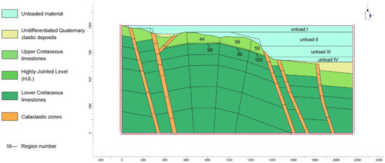
Figure 7.
Engineering-geological model used in the numerical analyses, showing the 102 regions identified, the different types of materials, and the boundary conditions considered. The model indicates the different unloading stages and the numbers of the regions for which the geomechanical characteristics are described in Table 3, Table 4 and Table 5. x-axis is in meters, while y-axis is in meters a.s.l.
The unit weight of each single region was estimated according to Discenza et al. [48], by considering different mass structures. For the intact rock constituting the jointed mass, the unit weight derived from the laboratory test was utilized. The jointed mass involved in DSGSD was characterized by measuring the discontinuities sets’ attitude and a unit weight of 20.0 kN/m3 for joint infilling material and 0.0 kN/m3 for an empty joint. Discontinuities were considered to be progressively more closed towards the bottom in relation to the lithostatic stress. For the cataclastic zones, astride to the faults, a unit weight of 20.0 kN/m3 was considered for the fine matrix present inside the rock blocks. The matrix was estimated to be 10% in the most superficial horizons and progressively less at depth. For the recent soil covers on the slope and the lacustrine sequence in the central portion of the Fucino plain, a unit weight of 20.0 kN/m3 was considered.
The rock mass strength was computed through the upgraded Hoek–Brown failure criterion [45], considering the results of the laboratory test and the GSI values derived from geomechanical surveys. The mi parameter was considered equal to 12 for all the calcareous lithotypes. Starting from the value measured at the surface, the GSI was increased by 5 every 100 m of depth, in order to simulate the improvement of characteristics due to the confining stress. In the jointed mass, the GSI was increased up to the maximum value of 80, while in the cataclastic zones the GSI was increased up to 50. In the calculation of tensile strength, the approach of Hoek–Martin [50] was used always, considering a mi parameter of 12. Recent covers, lacustrine deposits, marginal regions, and a very deep portion of rock mass were considered as perfectly elastic, in order to not have localized ruptures which have little influence on the analysis of the slope process.
Regarding the elastic parameters, in this case, the rock mass was also characterized by using the laboratory data and considering the jointing conditions observed on site. The Poisson ratio was adopted equal to those measured in UCS tests, while the Young modulus was calculated according to Sitharam et al. [43]. For each region in the model, the vertical load was determined at the central point, while the horizontal pressure was estimated by using the considered K0. The rock mass strength r was computed assuming filled joints at the surface and joints without infilling below 200 m of depth. To assign the joint dip n, the presence of bedding planes was considered in rock mass, while high angle discontinuities were considered for a cataclastic zone. The Jv parameter was determined through the spacing of joint sets, making it slightly decrease with depth to account for the increase in thickness of bedding planes and the decrease in jointing conditions. Both the Bulk and shear moduli were computed by using the previously described equation [9,10] through the Young modulus derived from the Sitharam approach.
The rheological properties of the rock mass were estimated through the equation of Discenza et al. [17], as it nowadays represents the only available equivalent continuum approach for the evaluation of time-dependent behavior of a jointed material starting from the characteristic of the rock matrix and discontinuities. For jointed limestones, the joint dip was considered equal to the dip of each region, while for the cataclastic zone the dip was taken as always equal to 60°. In the upper limestone sequence (Figure 7), an average bedding spacing of 50 cm was assumed, while in the lower limestone sequence a greater thickness of 150 cm (equal to the upper limit of the chosen approach) was considered. In cataclastic zones, the considered joint spacing was always of 15 cm, resulting from geomechanical surveyings, while in the HJL the spacing was considered as 10 cm. The time-dependent behavior of the mass was simulated through the rheological model of Burgers (Figure 8).
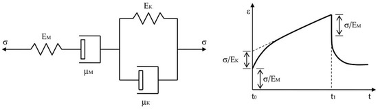
Figure 8.
Burgers visco-plastic rheological model and related time-dependent behavior in relation to the considered parameters.
The viscosity of intact limestones was attributed based on the literature data for similar rock masses [17,20] and assumed to be about 2.00 × 10¹⁹ Pa·s. Instead, the viscosity of the rock matrix in the HJL at the base of the Upper Cretaceous limestones was determined through a sensitivity analysis in a numerical model, by varying the parameters along the slope as a function of Discenza et al.’s [17] equation. This viscosity value, of about 2.00 × 10¹⁷ Pa·s, is lower with respect to the one attributed to rock mass. The viscosity for the Kelvin rheological element referring to the jointed rock was considered equal to the parameter determined with the described equation, while the viscosity of the Maxwell rheological element was assumed to be one order of magnitude lower with respect to the previous one. The Bulk modulus and the shear modulus for the Maxwell rheological element derive directly from the Young modulus calculated through the approach of Sitharam et al. [43], while the shear modulus for the Kelvin component was considered 1.2 times higher than the Maxwell rheological element.
In the upper portion of the slope, joint conditions were also considered in the numerical models. Regarding the joint strength, the parameters used in the Barton–Bandis model [54] were determined through the geomechanical survey conducted on the slope involved in the gravitational deformation. In particular, the JCS was calculated by using the Schmidt hammer rebound on discontinuity walls, while JRC was determined through an in situ test on joints. R and r numbers were calculated by using the same survey on both unweathered and weathered joint walls. All these parameters were determined separately for the jointed mass and the HJL.
The geometrical characteristic of the discontinuities set derives from a geomechanical survey and represents the mean values of dips and orientations of fractures inside the deforming rock mass. One set, relative to bedding planes, was considered for the HJL; two sets, relative to high angle joints connected with the tectonic setting of the slope, were used for the Upper Cretaceous limestone sequence. The discontinuity behavior was considered only for the shallowest regions, while it was not taken into account for the deepest regions (where the role of discontinuity is less important for the development of DSGSD) and for cataclastic zones (where the jointing conditions do not allow to assume the control of one or few joint sets).
5.2. Calculation Stages and Physical-Mechanical Parameters
Based on the geological-evolutionary model (Figure 4), different stages were developed in the numerical model. These stages allow to simulate the progressive debuttressing of the slope and the consequent variation of the stress-strain state of the rock mass. Considering the information available on the development of the DSGSD, time-dependent rheological models were applied only in the last stages of analyses. A calculation time of 90,000 years was applied to the Late Pleistocene phase, while a calculation time of 30,000 years was applied to the Latest Pleistocene – Holocene phase following the indication in Di Luzio et al. [39]. To limit calculation errors associated with the removal of large volumes of rock, the upper part of the mass present at the beginning of the Late Pleistocene was removed before the time-dependent analyses.
Table 3.
Synthesis of physical and strength parameters used for the rock mass. In this table, only the characteristics of the regions directly involved in DSGSD are reported. For location of different regions, please refer to Figure 7.
Table 3.
Synthesis of physical and strength parameters used for the rock mass. In this table, only the characteristics of the regions directly involved in DSGSD are reported. For location of different regions, please refer to Figure 7.
| Region | Lithology | Model | Unit Weight | Geological Strength Index | UCS Strength | Intact Rock Constant |
|---|---|---|---|---|---|---|
| - | - | - | γ | GSI | σc | mi |
| - | - | - | kN/m3 | - | MPa | - |
| 44 | Upper Cretaceous limestones | Burgers/Hoek-Brown | 25.9 | 50 | 82.4 | 12 |
| 56 | Upper Cretaceous limestones | Burgers/Hoek-Brown | 25.9 | 50 | 82.4 | 12 |
| 59 | Upper Cretaceous limestones | Burgers/Hoek-Brown | 25.9 | 50 | 82.4 | 12 |
| 98 | Highly-Jointed Level (HJL) | Burgers/Hoek-Brown | 25.6 | 35 | 24.9 | 12 |
| 99 | Highly-Jointed Level (HJL) | Burgers/Hoek-Brown | 25.6 | 35 | 24.9 | 12 |
| 100 | Highly-Jointed Level (HJL) | Burgers/Hoek-Brown | 25.6 | 35 | 24.9 | 12 |
The previously described parameters, together with the continuous and discontinuous physical-mechanical models, allowed us to characterize the 102 regions in which the section has been divided. All regions have been characterized with an equivalent continuum approach, while only to the shallow regions directly affected by the DSGSD discontinuous systems have been applied to simulate the joints sets. The physical and mechanical parameters of rock mass are reported in Table 3 and Table 4, while the main characteristics of joint sets are summarized in Table 5. For simplicity, only the characteristics of the regions directly affected by the deformation process are shown in these tables.
Table 4.
Synthesis of elastic and viscous parameters used for the rock mass. In this table, only the characteristics of the regions directly involved in DSGSD are reported. For location of different regions, please refer to Figure 7.
Table 4.
Synthesis of elastic and viscous parameters used for the rock mass. In this table, only the characteristics of the regions directly involved in DSGSD are reported. For location of different regions, please refer to Figure 7.
| Region | Lithology | Model | Young Modulus | Bulk Modulus | Shear Modulus Maxwell | Shear Modulus Kelvin | Poisson Ratio | Viscosity Maxwell | Viscosity Kelvin |
|---|---|---|---|---|---|---|---|---|---|
| - | - | - | E | K | G1 | G2 | υ | μM | μK |
| - | - | - | MPa | MPa | MPa | MPa | - | Pa·s | Pa·s |
| 44 | Upper Cretaceous limestones | Burgers/Hoek-Brown | 23,217 | 14,883 | 9362 | 11,234 | 0.24 | 3.08 × 10¹⁷ | 3.08 × 10¹⁸ |
| 56 | Upper Cretaceous limestones | Burgers/Hoek-Brown | 18,279 | 11,717 | 7371 | 8845 | 0.24 | 3.05 × 10¹⁷ | 3.05 × 10¹⁸ |
| 59 | Upper Cretaceous limestones | Burgers/Hoek-Brown | 6949 | 4454 | 2802 | 3362 | 0.24 | 3.03 × 10¹⁷ | 3.03 × 10¹⁸ |
| 98 | Highly-Jointed Level (HJL) | Burgers/Hoek-Brown | 12,540 | 8038 | 5056 | 6068 | 0.24 | 2.04 × 10¹⁵ | 2.04 × 10¹⁶ |
| 99 | Highly-Jointed Level (HJL) | Burgers/Hoek-Brown | 6954 | 4458 | 2804 | 3365 | 0.24 | 2.04 × 10¹⁵ | 2.04 × 10¹⁶ |
| 100 | Highly-Jointed Level (HJL) | Burgers/Hoek-Brown | 1851 | 1187 | 746 | 896 | 0.24 | 2.04 × 10¹⁵ | 2.04 × 10¹⁶ |
Table 5.
Synthesis of physical and mechanical parameters used for the joint sets. In this table, only the characteristics of the regions directly involved in DSGSD are reported. For location of different regions, please refer to Figure 7.
Table 5.
Synthesis of physical and mechanical parameters used for the joint sets. In this table, only the characteristics of the regions directly involved in DSGSD are reported. For location of different regions, please refer to Figure 7.
| Region | Lithology | Type | Dip | Model | Joint Wall Compressive Strength | Joint Roughness Coefficient |
|---|---|---|---|---|---|---|
| - | - | - | α | - | JCS | JRC |
| - | - | - | ° | - | MPa | - |
| 44 | Upper Cretaceous limestones | Fracture | 60 | Barton–Bandis | 25 | 9 |
| Fracture | 75 | Barton–Bandis | 30 | 10 | ||
| 56 | Upper Cretaceous limestones | Fracture | 70 | Barton–Bandis | 30 | 10 |
| Fracture | 70 | Barton–Bandis | 30 | 10 | ||
| 59 | Upper Cretaceous limestones | Fracture | 75 | Barton–Bandis | 30 | 10 |
| Fracture | 70 | Barton–Bandis | 30 | 10 | ||
| 98 | Highly-Jointed Level (HJL) | Bedding | 1 | Barton–Bandis | 20 | 9 |
| 99 | Highly-Jointed Level (HJL) | Bedding | 14 | Barton–Bandis | 20 | 9 |
| 100 | Highly-Jointed Level (HJL) | Bedding | 20 | Barton–Bandis | 20 | 9 |
5.3. Numerical Model Results
The numerical modeling allows us to reconstruct the evolution of the Luco dei Marsi DSGSD during the various stages of slope lateral unconfinement (since Early-Middle Pleistocene), and, in particular, during the Latest Pleistocene–Holocene period. The results showed the ongoing deformational process following the opening of the Fucino Basin, essentially due to visco-plastic deformations of the jointed rock mass and of the main joint sets. In all stages, a fundamental role was played by the inherited structures and particularly the level of HJL found in the lower section of the Upper Cretaceous carbonates sequence.
The outputs highlight a complete development of the deformational process, with displacement clearly directed towards the plain in the last stages (Figure 9). This evolution has led to the development of several yielded points/zones, both within the rock mass and along the main joint sets (Figure 10). Widespread failure conditions are found both on the surface (due to the unloading in the upper portion of the slope) and at the toe of the slope (due to the unloading and the ongoing of the gravitational deformation). Several yielded nodes are present along the HJL at the bottom of the slope, confirming the role of this level in the development of the BSZ. Another zone of high strain concentration corresponds to the axial area of the fold, where the gravitational grabens that characterize the slope are currently developed.
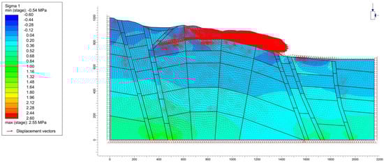
Figure 9.
Sigma 1 and displacement vectors during the last tectonic unloading (30,000 ya). x-axis is in meters, while y-axis is in meters a.s.l.
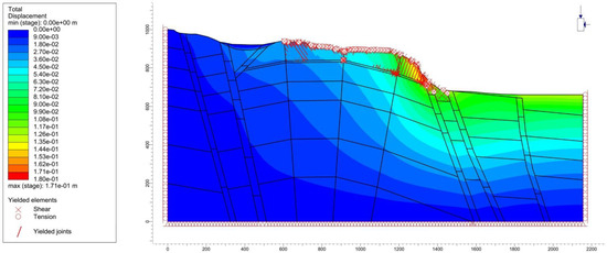
Figure 10.
Total displacement and yielded nodes/joints in the present conditions, after all unloading stages and creep evolution. x-axis is in meters, while y-axis is in meters a.s.l.
Regarding the joint sets (Figure 11), the model shows an arrangement that reflects the main characteristics of the deformational process detected through field surveys. Many ruptures are located at the surface and in the lower part of the slope, where the morphology of the ridge favors the development of several secondary and shallow landslides. Significant yielded joints are present in the upper portion of the slope, where they constitute the main shear zone of the deformational process. The most important failures are present at the base of the DSGSD, in correspondence with the HJL, which in the model includes the BSZ. In this case, the failures occur along the bedding planes in the anticline forelimb, which therefore control the evolution of the deformational process, especially in the outermost portion of the slope.
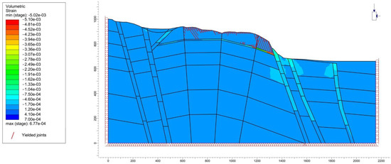
Figure 11.
Volumetric strain and yielded joints in the present condition, after all unloading stages and creep evolution. x-axis is in meters, while y-axis is in meters a.s.l.
6. Discussion
The numerical modeling performed on the cross-section across the slope involved in the Luco dei Marsi DSGSD allowed us to analyze the deformational process, reconstructing its kinematics, the different evolutionary phases, and the main control factors. The modeling results are consistent with the geomorphological evidence outlined for the DSGSD through field surveys, photo-interpretative analyses, geomechanical surveys, and interferometric monitoring [39]. The main geomorphological and kinematic elements of the deformation are highlighted through the modeling, while the strong control of pre-existing and inherited structural elements represents a necessary starting point for the development of the models.
The yielded nodes point out the main shallow and deep geomorphological and kinematic elements of the DSGSD (Figure 12). In the upper, western portion of the slope, the joint set dipping towards the Fucino Basin favors the development of the main shear zone and of the downhill-facing secondary planes. In the central portion, the different joint sets and the stress-strain condition along the fold axis led to the development of an extensive failure zone corresponding to the main gravitational grabens observed within the DSGSD (Figure 5 and Figure 6b). In the external sector of the slope, near the eastern margin of the ridge, yielded nodes are frequent both within the rock mass and along joint sets. This favors the surficial collapses at toe to which landslides mainly of the rock-fall type are linked [38].
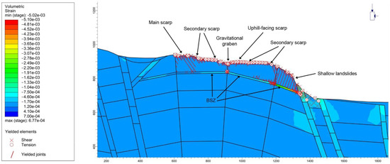
Figure 12.
Numerical modeling results (volumetric strain and yielded nodes/joints) with indication of the main geomorphological features and kinematic elements constraining the DSGSD process. x-axis is in meters, while y-axis is in meters a.s.l.
The presence of the HJL, about 10 m thick, at the base of the Upper Cretaceous limestones controls the evolution of the ridge and favors the development of the ongoing deformational process. Along this layer, several yielded nodes are present on both rock mass and joint set, mainly in the lower—external—portion of the slope where bedding planes present a high dip. The concentration of failures and shear/volumetric strain in this level (Figure 11 and Figure 12) confirms that the BSZ characterizing the Luco dei Marsi DSGSD was probably developed in correspondence with an already existing highly-jointed lithological horizon.
The calculation stages were defined according to the morpho-evolutionary model reconstructed for the Luco dei Marsi ridge (Figure 4). The model was run under creep configuration only in the last stages of the analysis, after the partial unloading of the slope. Such a sequential modeling reproduced the main evolutionary stages of the DSGSD process as well as the ongoing deformations over time (Figure 13). During the first unloading stages (initial condition up to the Early-Middle Pleistocene, step I in Figure 4), no noteworthy deformation elements were generated (Figure 13a,b). Starting from the third phase (Latest Middle Pleistocene, step II in Figure 4), the progressive debuttressing of the slope caused by the embryonic normal faulting favors the formation of a few failure points along the pre-existing HJL, and in correspondence with the faults bordering the opening basin (Figure 13c).
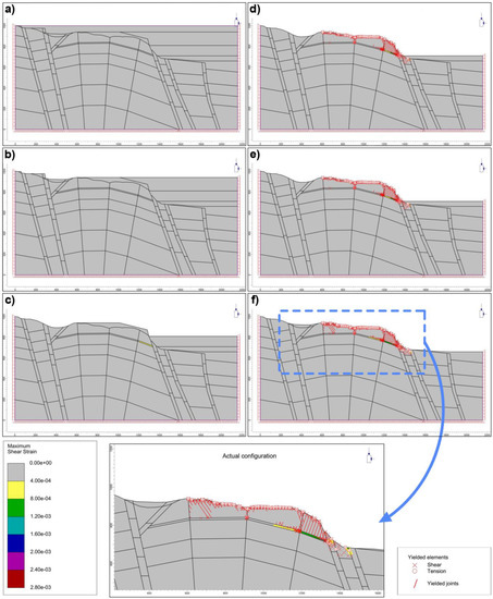
Figure 13.
Evolutionary model, maximum shear strain, and yielded nodes/joints along the modeled section: (a) Initial condition; (b) Early-Middle Pleistocene; (c) Latest Middle Pleistocene; (d) Latest Pleistocene; (e) Latest Pleistocene after partial slope unloading; (f) Holocene. Visco-plastic deformations were applied to stage (e) (90,000 years) and (f) (30,000 years). x-axis is in meters, while y-axis is in meters a.s.l.
In the following stage (Late Pleistocene, step III in Figure 4), the significant unloading of the slope leads to the formation of widespread yielded elements along the fractured level and at the base of the slope, in correspondence with the toe of the current deformation (Figure 13d). This condition, together with the variation of the stress-strain state of the mass, favors the creep process (still Late Pleistocene) which drives the formation of a widespread state of plasticization both on the surface and inside the mass (Figure 13e) in about 90,000 years. Finally, the last unloading phase (Holocene, step IV in Figure 4) and the progress of the creep processes—after about 30,000 years—lead to the full development of the DSGSD process and to the formation of the main geomorphological and kinematic elements (Figure 13f), such as main scarp, secondary downhill- and uphill-facing scarps, gravitational grabens, trenches, and secondary landslides.
The numerical modeling demonstrated that both the BSZ and the shallow features were formed progressively over time because of an ongoing damaging process. Their development was controlled both by the slope debuttressing phases due to normal faulting and by the progress of the viscosity-driven process. The latter, even if it has not produced significant displacements, has favored the variation of the stress-strain state of the rock mass and the progressive plasticization of some sectors for the achievement of tertiary creep. The displacements computed in the calculation stages resulted in the order of a few millimeters or, at most, a few centimeters. The differences with respect to the strains recorded through interferometric analyzes of geomorphological studies—of the order of a few mm/yr [39]—can be related to plastic strains (mainly occurring along the joints), for which displacement cannot be analyzed using the here performed simulation approach.
7. Conclusions
The stress-strain numerical modeling performed for the Luco dei Marsi DSGSD allowed us to define the main control factors of the gravitational deformation, the rheological behavior of the rock mass, and the resulting deformational mechanism. The engineering-geological model of the slope was reconstructed based on field surveys, geomorphological analyses, photo-interpretative studies, and interferometric analyses. The physical and mechanical properties of the rock mass and of the main joint sets were derived from geomechanical surveys and laboratory tests on intact rock samples. The sequential analysis was based on a previous reconstructed geological-evolutionary model of the Luco dei Marsi ridge. An equivalent continuous approach of jointed rock was used together with a discontinuous joint model for analyzing the visco-plastic behavior of the rock mass.
The numerical model outputs showed that the Luco dei Marsi DSGSD has been strongly influenced: (i) by the different stages of unloading that have occurred over time caused by normal faulting with different rates and (ii) by the inherited and pre-existing elements (joints, highly-fractured levels, and fold features) present along the slope. Several kinematic elements correspond to the high angle joint sets surveyed in the upper part of the slope, especially in the top-ridge area and at the base of the relief. The BSZ instead progressively formed along the HJL- about 10 m thick—present in the lower section of the Upper Cretaceous carbonate sequence making the backbone of the ridge. All these elements, favored by the creep processes in the rock mass and by the plastic deformations along the joints, have led to the development of the gravitational process and to the formation of the geomorphological features which can be observed along the Luco dei Marsi ridge.
Author Contributions
Conceptualization, M.E.D., E.D.L. and S.M.; methodology, M.E.D. and S.M.; software, M.E.D., M.M. and S.M.; validation, M.E.D., E.D.L. and S.M.; formal analysis, M.E.D. and E.D.L.; investigation, E.D.L.; data curation, M.E.D.; writing—original draft preparation, M.E.D. and E.D.L.; writing—review and editing, M.E.D. and E.D.L.; visualization, M.M.; supervision, S.M. and C.E.; funding acquisition, C.E. All authors have read and agreed to the published version of the manuscript.
Funding
This research was funded by the Sapienza University of Rome (research project “Integrated analysis and hazard-oriented modeling of large-scale slope instabilities featured by Mass Rock Creep—Scientific responsible Carlo Esposito”—prot. RG11916B88FA477F).
Data Availability Statement
The data presented in this study are available on request from the author. The data are not publicly available due to privacy reasons.
Acknowledgments
The authors are thankful to local public authorities for logistic support.
Conflicts of Interest
The authors declare no conflict of interest.
References
- Jaboyedoff, M.; Penna, I.; Pedrazzini, A.; Baroň, I.; Crosta, G.B. An introductory review on gravitational-deformation induced structures, fabrics and modeling. Tectonophysics 2013, 605, 1–12. [Google Scholar] [CrossRef]
- Bozzano, F.; Della Seta, M.; Martino, S. Time-dependent evolution of rock slopes by a multi-modelling approach. Geomorphology 2016, 263, 113–131. [Google Scholar] [CrossRef]
- Pánek, T.; Klimeš, J. Temporal behavior of deep-seated gravitational slope deformations: A review. Earth-Sci. Rev. 2016, 156, 14–38. [Google Scholar] [CrossRef]
- Discenza, M.E.; Esposito, C. State-of-art and remarks on some open questions about DSGSDs: Hints from a review of the scientific literature on related topics. Ital. J. Eng. Geol. Environ. 2021, 21, 31–59. [Google Scholar] [CrossRef]
- Di Martire, D.; Novellino, A.; Ramondini, M.; Calcaterra, D. A-differential synthetic aperture radar interferometry analysis of a deep seated gravitational slope deformation occurring at Bisaccia (Italy). Sci. Total Environ. 2016, 550, 556–573. [Google Scholar] [CrossRef] [PubMed]
- Delchiaro, M.; Della Seta, M.; Martino, S.; Dehbozorgi, M.; Nozaem, R. Reconstruction of river valley evolution before and after the emplacement of the giant Seymareh rock avalanche (Zagros Mts., Iran). Earth Surf. Dyn. 2019, 7, 929–947. [Google Scholar] [CrossRef]
- Jarman, D.; Harrison, S. Rock slope failure in the British mountains. Geomorphology 2019, 340, 202–233. [Google Scholar] [CrossRef]
- Discenza, M.E.; Esposito, C.; Komatsu, G.; Miccadei, E. Large-Scale and Deep-Seated Gravitational Slope Deformations on Mars: A Review. Geosciences 2021, 11, 174. [Google Scholar] [CrossRef]
- Delchiaro, M.; Della Seta, M.; Martino, S.; Nozaem, R.; Moumeni, M. Tectonic deformation and landscape evolution inducing mass rock creep driven landslides: The Loumar case-study (Zagros Fold and Thrust Belt, Iran). Tectonophysics 2023, 846, 229655. [Google Scholar] [CrossRef]
- Chigira, M. Long-term gravitational deformation of rocks by mass rock creep. Eng. Geol. 1992, 32, 157–184. [Google Scholar] [CrossRef]
- Hippolyte, J.C.; Brocard, G.; Tardy, M.; Nicoud, G.; Bourles, D.; Braucher, R.; Ménard, G.; Souffaché, B. The recent fault scarps of the Western Alps (France): Tectonic surface ruptures or gravitational sackung scarps? A combined mapping, geomorphic, levelling, and 10Be dating approach. Tectonophysics 2006, 418, 255–276. [Google Scholar] [CrossRef]
- Bozzano, F.; Martino, S.; Montagna, A.; Prestininzi, A. Back analysis of a rock landslide to infer rheological parameters. Eng. Geol. 2012, 131, 45–56. [Google Scholar] [CrossRef]
- Esposito, C.; Di Luzio, E.; Scarascia Mugnozza, G. Mutual interactions between slope-scale gravitational processes and morpho-structural evolution of central Apennines (Italy): Review of some selected case histories. Rend. Fis. Acc. Lincei 2014, 25, 151–165. [Google Scholar] [CrossRef]
- Alfaro, P.; Delgado, J.; Esposito, C.; Tortosa, G.F.; Marmoni, G.M.; Martino, S. Time-dependent modelling of a mountain front retreat due to a fold-to-fault controlled lateral spreading. Tectonophysics 2019, 773, 228233. [Google Scholar] [CrossRef]
- Esposito, C.; Di Luzio, E.; Baleani, M.; Troiani, F.; Della Seta, M.; Bozzano, F.; Mazzanti, P. Fold architecture predisposing deep-seated gravitational slope deformations within a flysch sequence in the Northern Apennines (Italy). Geomorphology 2021, 380, 107629. [Google Scholar] [CrossRef]
- Della Seta, M.; Esposito, C.; Marmoni, G.M.; Martino, S.; Scarascia Mugnozza, G.; Troiani, F. Morpho-structural evolution of the valley-slope systems and related implications on slope-scale gravitational processes: New results from the Mt. Genzana case history (Central Apennines, Italy). Geomorphology 2017, 289, 60–77. [Google Scholar] [CrossRef]
- Discenza, M.E.; Martino, S.; Bretschneider, A.; Scarascia Mugnozza, G. Influence of joints on creep processes involving rock masses: Results from physical-analogue laboratory tests. Int. J. Rock Mech. Min. Sci. 2020, 128, 104261. [Google Scholar] [CrossRef]
- Vick, L.M.; Böhme, M.; Rouyet, L.; Bergh, S.G.; Corner, G.D.; Lauknes, T.R. Structurally controlled rock slope deformation in northern Norway. Landslides 2020, 17, 1745–1746. [Google Scholar] [CrossRef]
- Martino, S.; Prestininzi, A.; Scarascia Mugnozza, G. Geological-evolutionary model of a gravity-induced slope deformation in the carbonate Central Apennines (Italy). Q. J. Eng. Geol. Hydrogeol. 2004, 37, 31–47. [Google Scholar] [CrossRef]
- Discenza, M.E.; Esposito, C.; Martino, S.; Petitta, M.; Prestininzi, A.; Scarascia Mugnozza, G. The gravitational slope deformation of Mt. Rocchetta ridge (central Apennines, Italy): Geological-evolutionary model and numerical analysis. Bull. Eng. Geol. Environ. 2011, 70, 559–575. [Google Scholar] [CrossRef]
- Carbonel, D.; Gutiérrez, F.; Linares, R.; Roqué, C.; Zarroca, M.; McCalpin, J.; Guerrero, J.; Rodríguez, V. Differentiating between gravitational and tectonic faults by means of geomorphological mapping, trenching and geophysical surveys. The case of the Zenzano Fault (Iberian Chain, N Spain). Geomorphology 2013, 189, 93–108. [Google Scholar] [CrossRef]
- Di Luzio, E.; Saroli, M.; Esposito, C.; Bianchi-Fasani, G.; Cavinato, G.P.; Scarascia Mugnozza, G. Influence of structural framework on mountain slope deformation in the Maiella anticline (Central Apennines, Italy). Geomorphology 2004, 60, 417–432. [Google Scholar] [CrossRef]
- Esposito, C.; Martino, S.; Scarascia Mugnozza, G. Mountain slope deformations along thrust fronts in jointed limestone: An equivalent continuum modelling approach. Geomorphology 2007, 90, 55–72. [Google Scholar] [CrossRef]
- Moro, M.; Saroli, M.; Tolomei, C.; Salvi, S. Insights on the kinematics of deep-seated gravitational slope deformations along the 1915 Avezzano earthquake fault (Central Italy), from time-series DInSAR. Geomorphology 2009, 112, 261–276. [Google Scholar] [CrossRef]
- Bianchi Fasani, G.; Di Luzio, E.; Esposito, C.; Evans, S.G.; Scarascia Mugnozza, G. Quaternary, catastrophic rock avalanches in the Central Apennines (Italy): Relationships with inherited tectonic features, gravity-driven deformations and the geodynamic frame. Geomorphology 2014, 211, 22–42. [Google Scholar] [CrossRef]
- Zischinsky, U. On the deformation of high slopes. In Proceedings of the 1st Conference of the International Society of Rock Mechanics, Lisbon, Portugal, 25 September–1 October 1966; Volume 2, pp. 179–185. [Google Scholar]
- Radbruch-Hall, D. Gravitational creep of rock masses slopes. In Rockslides and Avalanches Natural Phenomena; Development in Geotechnical Engineering; Voight, B., Ed.; Elsevier: Amsterdam, The Netherlands, 1978; pp. 607–657. [Google Scholar]
- Hutchinson, J.N. General report: Morphological and geotechnical parameters of landslides in relation to geology and hydrogeology. In Proceedings of the 5th International Symposium on Landslides, Lausanne, Switzerland, 10–15 July 1988; Volume 1, pp. 3–35. [Google Scholar] [CrossRef]
- Emery, J.Z. Simulation of slope creep. In Rockslides and Avalanches Natural Phenomena; Development in Geotechnical Engineering; Voight, B., Ed.; Elsevier: Amsterdam, The Netherlands, 1978; pp. 669–691. [Google Scholar]
- Apuani, T.; Masetti, M.; Rossi, M. Stress-strain-time numerical modelling of a deep-seated gravitational slope deformation: Preliminary results. Quat. Int. 2007, 171–172, 80–89. [Google Scholar] [CrossRef]
- Bianchi Fasani, G.; Di Luzio, E.; Esposito, C.; Martino, S.; Scarascia Mugnozza, G. Numerical modelling of Plio-Quaternary slope evolution based on geological constraints: A case study from the Caramanico Valley (Central Apennines, Italy). Geol. Soc. Lond., Spec. Publ. 2011, 351, 201–214. [Google Scholar] [CrossRef]
- Hou, Y.L.; Chigira, M.; Tsou, C.Y. Numerical study on deep-seated gravitational slope deformation in a shale-dominated dip slope due to river incision. Eng. Geol. 2014, 179, 59–75. [Google Scholar] [CrossRef]
- Leith, K.; Moore, J.R.; Amann, F.; Loew, S. Subglacial extensional fracture development and implications for Alpine Valley evolution. J. Geophys. Res. Earth Surf. 2014, 119, 62–81. [Google Scholar] [CrossRef]
- Bois, T.; Zerathe, S.; Lebourg, T.; Tric, E. Analysis of lateral rock spreading process initiation with a numerical modelling approach. Terra Nova 2018, 30, 369–379. [Google Scholar] [CrossRef]
- Chalupa, V.; Pánek, T.; Šilhán, K.; Břežný, M.; Tichavský, R.; Grygar, R. Low-topography deep-seated gravitational slope deformation: Slope instability of flysch thrust fronts (Outer Western Carpathians). Geomorphology 2021, 389, 107833. [Google Scholar] [CrossRef]
- Makowska, M.; Mège, D.; Gueydan, F.; Chéry, J. Mechanical conditions and modes of paraglacial deep-seated gravitational spreading in Valles Marineris, Mars. Geomorphology 2016, 268, 246–252. [Google Scholar] [CrossRef]
- De Blasio, F.V.; Martino, S. The Acheron Dorsum on Mars: A novel interpretation of its linear depressions and a model for its evolution. Earth Planet. Sci. Lett. 2017, 465, 92–102. [Google Scholar] [CrossRef]
- Di Luzio, E.; Schilirò, L.; Gaudiosi, I. Cultural Heritage and Rockfalls: Analysis of Multi-Scale Processes Nearby the Lucus Angitiae Archaeological Site (Central Italy). Geosciences 2021, 12, 521. [Google Scholar] [CrossRef]
- Di Luzio, E.; Discenza, M.E.; Di Martire, D.; Putignano, M.L.; Minnillo, M.; Esposito, C.; Scarascia Mugnozza, G. Investigation of the Luco dei Marsi DSGSD revealing the first evidence of a basal shear zone in the Central Apennine belt (Italy). Geomorphology 2022, 408, 108249. [Google Scholar] [CrossRef]
- Cavinato, G.P.; Carusi, C.; Dall’Asta, M.; Miccadei, E.; Piacentini, T. Sedimentary and tectonic evolution of Plio-Pleistocene alluvial and lacustrine deposits of Fucino Basin (central Italy). Sedim. Geol. 2002, 148, 29–59. [Google Scholar] [CrossRef]
- Patacca, E.; Scandone, P.; Di Luzio, E.; Cavinato, G.P.; Parotto, M. Structural architecture of the central Apennines. Interpretation of the CROP 11 seismic profile from the Adriatic coast to the orographic divide. Tectonics 2008, 27, TC3006. [Google Scholar] [CrossRef]
- Martino, S.; Di Luzio, E.; Discenza, M.E.; Esposito, C.; Minnillo, M. Dataset on physical properties and mechanical parameters of limestone in Central Apennine (Italy) derived from laboratory test on intact rocky specimens. Data Brief 2023, 46, 108886. [Google Scholar] [CrossRef]
- Sitharam, T.G.; Sridevi, J.; Shimizu, N. Practical equivalent continuum characterization of jointed rock masses. Int. J. Rock Mech. Min. Sci. 2001, 38, 437–448. [Google Scholar] [CrossRef]
- Amadei, B.; Swolfs, H.S.; Savage, W.Z. Gravity-induced stresses in stratified rock masses. Rock Mech. Rock Eng. 1988, 21, 1–20. [Google Scholar] [CrossRef]
- Hoek, E.; Carranza-Torres, C.T.; Corkum, B. Hoek-Brown failure criterion—2002 edition. In Mining Innovation and Technology, Proceedings of the 5th North American Rock Mechanics Symposium, Salt Lake City, UT, USA, 27–30 June 2010; Bawden, H.R.W., Curran, J., Telsenicki, M., Eds.; University of Toronto Press: Toronto, ON, Canada, 2002. [Google Scholar]
- Zhang, L.; Einstein, H.H. Using RQD to estimate the deformation modulus of rock masses. Int. J. Rock Mech. Min. Sci. 2004, 41, 337–341. [Google Scholar] [CrossRef]
- Ramamurthy, T.; Latha, G.M.; Sitharam, T.G. Modulus Ratio and Joint Factor concepts to predict rock mass response. Rock Mech. Rock Eng. 2017, 50, 353–366. [Google Scholar] [CrossRef]
- Discenza, M.E.; De Pari, P.; Kundu, J.; Minnillo, M.; Romano, S.; Scarascia Mugnozza, G. Innovative approach for the determination of unit weight and density of soil and rock masses. Ital. J. Eng. Geol. Environ. 2021, 21, 61–76. [Google Scholar] [CrossRef]
- Hoek, E.; Marinos, P. GSI: A geologically friendly tool for rock mass strength estimation. In Proceedings of the International Conference on Geotechnical and Geological Engineering, Melbourne, Australia, 19–24 November 2000. [Google Scholar]
- Hoek, E.; Martin, C.D. Fracture initiation and propagation in intact rock—A review. J. Rock Mech. Geotech. Eng. 2014, 6, 287–300. [Google Scholar] [CrossRef]
- Ramamurthy, T. Strength and modulus responses of anisotropic rocks. In Comprehensive Rock Engineering; Hudson, J.A., Ed.; Pergamon Press: Oxford, UK, 1994. [Google Scholar]
- Sridevi, J.; Sitharam, T.G. Analysis of strength and moduli of jointed rocks. Geotech. Geol. Eng. 2000, 18, 3–21. [Google Scholar] [CrossRef]
- Sitharam, T.G.; Latha, M.G. Simulation of excavations in jointed rock masses using a practical equivalent continuum approach. Int. J. Rock Mech. Min. Sci. 2002, 39, 517–525. [Google Scholar] [CrossRef]
- Barton, N.R.; Choubey, V. The shear strength of rock joints in the theory and practice. Rock Mech. 1977, 10, 1–54. [Google Scholar] [CrossRef]
- Rocscience, version RS2 v.11.015; Sapienza University of Rome: Rome, Italy, 2022.


Disclaimer/Publisher’s Note: The statements, opinions and data contained in all publications are solely those of the individual author(s) and contributor(s) and not of MDPI and/or the editor(s). MDPI and/or the editor(s) disclaim responsibility for any injury to people or property resulting from any ideas, methods, instructions or products referred to in the content. |
© 2023 by the authors. Licensee MDPI, Basel, Switzerland. This article is an open access article distributed under the terms and conditions of the Creative Commons Attribution (CC BY) license (https://creativecommons.org/licenses/by/4.0/).