Abstract
With the increase of service time, the rotation period of rotating machinery may become irregular, and the Ensemble Empirical Mode Decomposition (EEMD)can effectively reflect its periodic state. In order to accurately evaluate the working state of the Rotate Vector (RV) reducer, the torque transfer formula of the RV reducer is first derived to theoretically prove periodicity of torque transfer in normal operation. Then, EEMD is able to effectively reflect the characteristics of data periodicity. A fault diagnosis model based on EEMD-MPA-KELM was proposed, and a bearing experimental dataset from Xi‘an Jiaotong University was used to verify the performance of the model. In view of the characteristics of the industrial robot RV reducer fault was not obvious and the sample data is few, spectrum diagram was used to diagnose the fault from the RV reducer measured data. The EEMD decomposition was performed on the data measured by the RV reducer test platform to obtain several Intrinsic Mode Functions (IMF). After the overall average checking and optimization of each IMF, several groups of eigenvalues were obtained. The eigenvalues were input into the Kernel Extreme Learning Machine (KELM) optimized by the Marine Predators Algorithm (MPA), and the fault diagnosis model was established. Finally, compared with other models, the prediction results showed that the proposed model can judge the working state of RV reducer more effectively.
1. Introduction
The Rotate Vector (RV) reducer is a new type of cycloidal pinwheel planetary drive two-stage gear reducer, which is mainly applied in the field of robotics. With the increasing demand of industrial robots, the RV reducer, as a core parts in robots, plays a very important role in the actual production process. If the RV retarder fails, it will reduce the economic benefit of the manufacturer. Therefore, it is urgent to have a method of fault diagnosis and life prediction for the RV retarder to reduce losses caused by RV retarder failure.
In recent years, domestic and foreign scholars have done a lot of research on RV reducers. Pan Bosong [1] and others analyzed the reliability of transmission accuracy of planetary gear reducer considering gear wear. Li Zhe [2] and others placed sensors in multiple locations for data extraction and preprocessing, carried out preliminary processing, and introduced the analyzed information into the deep convolutional neural network, improving the accuracy and robustness of the existing fault diagnosis for the reducer. Wang Jiugen [3] input the data of different fault modes measured by the vibration test bench into the residual neural network for training and five-fold cross-validation, and then compared it with multiple neural network models, and verified it by using the database of Western Reserve University. Mao Jun [4] put forward a fault diagnosis method based on Deep Auto-Encoder Networks (DAENS), taking several common fault features of reducers as input and whether there was a fault or not as output. Peng [5] clearly proposed the entity model of a convolutional neural network under the influence of noise, converted the one-dimensional vibration data signal of the RV reducer into gray image after two-dimensional transformation, took it as input and fused the features. Chen Lerui [6] selected a method closely combining frequency bands and a large number of possible optimization algorithms according to the output phase frequency characteristic function and Kernel Principal Component Analysis (KPCA) of discrete systems, and obtained the first four frequency band values. In each case, SVM was introduced and compared with various diagnostic methods after the KPCA solution was used. An Haibo [7] analyzed the basic principle of the RV reducer dynamics and established the transmission model of the AE data signal inside RV reducer. Yu Ning [8] carried out CMF decomposition of fault signals, improved local Mean Decomposition (CELMD), and combined Multi-scale Perarrangement Entropy (MPE) method to select the PF component for reconstruction, envelope analysis and other comprehensive diagnosis methods. HM Qian [9] put forward a time-varying reliability method for an industrial robot Rotation Vector (RV) reducer with multiple failure modes using the Kriging model, and a time-varying reliability analysis method for multiple failure modes based on the double-ring Kriging model. The inner loop is the extreme value optimization of each limit state function based on Efficient Global Optimization (EGO), while the outer loop is the active learning reliability analysis combining the Multi-Response Gaussian Process model (MRGP) and Monte Carlo Simulation (MCS).
With the development of artificial intelligence, extreme learning machine, as a kind of pattern recognition, has been given wide attention due to its fast running speed and small amount of training data. Wang H. [10] adopted the extreme learning machine method to classify the faults of fuel system. Guo S. [11] combined the circle model with the Extreme Learning Machine (ELM) to form a fault diagnosis method for linear analog circuits. Xia Y. [12] reported an effective method for early fault diagnosis of a chiller by combining nuclear Entropy Component Analysis (KECA) and a Voting based Extreme Learning Machine (VELM). Liu X. [13] proposed a personalized fault diagnosis method using Finite Element Method (FEM) simulation and ELM to detect faults in gears. Huang [14] from Nanyang Technological University introduced a kernel function idea from a support vector machine into ELM to improve the stability and generalization ability of ELM neural network model training results, and proposed Kernel Extreme Learning Machine (KELM). Yang Xin [15] used the nuclear extreme learning machine to classify turbine rotor faults. Qiao Wenshan [16] proposed a fault diagnosis method based on IBOA-KELM to improve the accuracy and efficiency of diesel engine fault diagnosis. Liang R. [17] proposed a fault diagnosis method based on the Whale Optimization Algorithm (WOA) to optimize KELM, aiming at the problems that fault features are difficult to extract and time-frequency features cannot fully represent state information. Zhang H. [18] proposed a fault diagnosis method for the coal mill of a nuclear extreme learning machine based on feature extraction of a variational model. The above studies combined various methods with the nuclear extreme learning machine for fault diagnosis, and achieved good results, but most of them have poor universality. Moreover, because KELM introduced kernel functions, it is very sensitive to parameters and has randomness, so the results are not stable every time, which is easy to affect the prediction results.
The above fault diagnosis method for the RV reducer has a high accuracy, but the content of the method is more complex, with more complicated calculation, and a large number of data support is needed. Often, the data characteristics of the RV reducer are fewer when the initial fault occurs, resulting in the reduced accuracy of the RV reducer in operation, and the fault cannot be detected. In this paper, a MPA-KELM fault diagnosis and classification model for RV reducer of a small sample of industrial robots based on EEMD was proposed. In view of the characteristics of the industrial robot RV reducer where the fault is not obvious and the sample data are sparse, the spectrum diagram was used to diagnose the fault from the measured data of RV reducer, the data measured by the RV reducer test platform was decomposed by EEMD, and several Intrinsic Mode Functions (IMFs) are obtained. After the overall average checking and optimization of each IMF, multiple groups of characteristic values were obtained. The eigenvalues are imported as inputs into the KELM optimized by the Marine Predators Algorithm (MPA) in order to accurately evaluate the RV reducer working state and establish a fault diagnosis model.
2. Industrial Robot RV Reducer
RV Reducer Structure of Industrial Robots
As shown in Figure 1 [19], the RV reducer uses the solar wheel as the input shaft, and the solar wheel with fewer teeth drives the planetary wheel with more teeth to rotate, so as to carry out first-stage deceleration. The large planetary wheel drives the crank shaft to rotate, and the crank shaft drives two RV wheels to rotate, the two RV wheels rotate for one circle, and the pinion gear rotates for one tooth, so as to carry out second-stage deceleration.
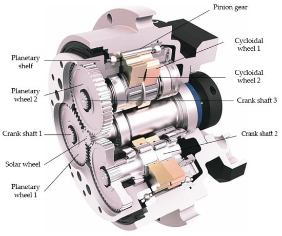
Figure 1.
Structure diagram of RV reducer of industrial robot.
Since the center of gravity of the crank shaft is not on the shaft, its torque will change periodically with rotation. The calculation formula is shown in Equation (1):
In the formula, —Crank shaft torque, kNm; —Torque factor, m; —Suspension instantaneous load, kN; —Crank structure unbalanced weight, kN; —Maximum crank balance torque, —Crank Angle; —Phase Angle.
Wp is the weight of the crank balance block, Rp is the distance between the crank shaft and the center of gravity of the balance block, Wb′ is the weight of the crank, and Rb is the distance between the crank shaft and the center of gravity.
Since the crank shaft of RV reducer does not need a crank balance block, the formula for RV reducer can be expressed as:
The torque factor can also be expressed as follows:
In formula, A is the length of the forearm of the traveling beam, B is the length of the rear arm of the traveling beam, d is the distance of the central crank shaft of the cycloidal wheel, α and β are the Angle between the connecting rod and the crank. Because does not have the RV reducer, connecting rod, the Angle α is zero, so the torque factor also is zero, so the type (1) can be simplified as:
While the center of the cycloidal wheel is not in line with the axis, assuming that the difference is s and the radius of the cycloidal wheel is r, the formula of the cycloidal wheel is:
When cycloidal wheel and pinion gear transfer torque, the torque needs to add a mesh coefficient C1.
Then its final output torque is:
Since the efficiency formula is:
In formula, n is the deceleration ratio.
From Formula (8), it can be concluded that the efficiency of RV reducer in normal operation is periodic.
3. Theoretical Basis
3.1. KELM
Extreme Learning Machine (ELM) is a neural network algorithm composed of single hidden layer. Because the hidden layer of the input weight kernel is randomly biased and fixed in the network, compared with the traditional neural network, the parameter setting is lower, the learning speed is faster, and the generalization ability is stronger.
Suppose that the input of the model’s training set is N-dimensional , the ideal output is I dimensional , when the number of hidden nodes L and the excitation function G(x) are determined, the calculation formula of the actual output value of ELM network is:
In formula, Wnl is the input weight between node n of ELM input layer and node l of hidden layer; bl is the bias of the l th hidden layer node; βli is the output weight of hidden layer node l and output layer node i. G(x) is the activation function.
When the input sample is trained by ELM network model, the output data can be infinitely approximated to an ideal output , there is a definite combination of W, b and β, such that Y = T, then the above formula can be converted into a matrix form:
In formula, H is the output matrix of the hidden layer; β is the weight matrix of the output layer; T is the expected output matrix.
Using the least square method to solve β, we can obtain:
In formula, H+ is the generalized inverse matrix of matrix H.
Due to the randomness of the setting of input layer weight and hidden layer bias in ELM, the state of the model is extremely unstable. Therefore, Huang and others from Nanyang Technological University introduced kernel function idea from the Support Vector Machine (SVM) into ELM and proposed Kernel Extreme Learning Machine (KELM). The algorithm not only has the same excellent running speed as the ELM neural network, but also has more stable performance and generalization ability as SVM. Kernel function is used to map the input space to higher dimensional space to enhance the stability of the model. That is, kernel function matrix ΩELM is used to replace E hidden layer random matrix HHT. Based on Mercer condition definition, we can obtain:
RBF kernel function is adopted in this paper:
In formula, σ is the width parameter of RBF kernel function.
The regularization coefficient C and the identity matrix I are introduced into the ELM neural network random matrix HHT, and the evaluation formula of β′ is as follows:
Based on the above formula, the output function of KELM neural network can be written:
3.2. MPA
The Marine Predators Algorithm (MPA) is a novel and efficient meta-heuristic algorithm proposed by Faramarzi [20] in 2020, which was mainly inspired by the motion laws of predators and prey in the ocean and the optimal encounter rate strategies for biological interactions between predators and prey. The optimization process is divided into three stages based on the speed scores of the predator and the prey, with the predator following a regular levy motion or Brownian motion. At the same time, the prey also acts as the predator identity while being hunted, making the algorithm more realistic in principle. In addition, considering the Marine environmental factors, it can reduce the phenomenon of predators falling into the local optimal value.
The detailed steps of MPA algorithm implementation are as follows:
- Initialize the Elite matrix and Prey matrix. Each element in the Prey matrix is initialized by a formula.
In formula, uj and lj are the upper and lower limits of the search space in the j dimension; rand is a random vector subject to uniform distribution [0,1], and Xij represents the j-dimensional spatial position of the i prey. The final Prey matrix is obtained:
In formula, n is the population size and d is the dimension value.
The fitness value of each predator was calculated, and the predator with the best fitness was selected to make n copies to form the Elite matrix:
In formula, n is the population size and d is the dimension value. The Elite matrix has the same dimension as the Predator matrix.
- 2.
- Optimization process. In the optimization process, there are three stages.
Stage 1: In the early iteration, the first third of the total iteration, the prey moves faster than the predator in this stage. The predator is mainly in the exploratory phase, and the optimal strategy is to be completely motionless. The mathematical model of this stage is:
In formula, si is the moving step; RB is a random vector with Brownian motion based on normal distribution; is term by term multiplication; R is a uniform random vector in [0,1]; t is the number of current iterations; T is the maximum number of iterations.
Stage 2: In the middle of the iteration, one-third to two-thirds of the way through the iteration, prey and predator are moving at the same speed. Predators are mainly in the exploration and development transition phase, so half of the predators are for exploration and the other half for development. At this point, the prey uses Levi’s Walk for exploitation and the predator uses Brownian motion for exploration. The mathematical model of this stage is:
In formula, RL is a random vector generated based on Levy distribution; CF is an adaptive parameter that controls the predator’s movement step size.
Stage 3: In the late iteration stage, the predator moves faster than the prey. The predator is in the development stage, and the best strategy is Levi’s walk. Its mathematical model is:
- 3.
- Fish Aggregation Device Effect (FADs).
In order to avoid the stagnation of local optimal value, MPA considers the influence of environmental factors such as fish aggregation device, and the mathematical model of FADs is as follows:
In formula, U is a random binary vector of an array containing 0 and 1; r1 and r2 are not random indexes of the prey matrix.
4. Establishment of RV Reducer Fault Diagnosis Model
4.1. EEMD Preprocessing
Empirical Mode Decomposition (EMD) is an empirical mode decomposition method that can reflect the instantaneous frequency of data, but since the input noise is generated randomly, it is easy to cause problems such as mode aliasing, end effect, and stop standard of screening iteration. To solve the above problems, Wu [21] and others proposed Ensemble Em-pirical Mode Decomposition (EEMD). The method solves the mode aliasing phenomenon by adding white noise to fill the discontinuous signal segment. In the process of noise signal decomposition, the filtering characteristics of white noise signal are used to solve the IMF average value for many times to eliminate the interference of white noise on the original signal at discontinuous points [22].
Data preprocessing steps are as follows [23]:
Step 1: Divide the fault data into several sample data, and add normal white noise Sw(ω) to each sample data x(t) to obtain a new overall xs(t).
The expression of normal white noise Sw (ω) is as follows:
In the formula, the expression of Rw (l) is as follows:
In the formula, the expression of δl is as follows:
Step 2: Perform EMD decomposition on xs (t), the sample data with white noise added, to obtain several IMF components. The flow chart is shown as follows:
In the formula, imfc(t) is the c IMF of EMD decomposition. rn(t) is the participating weight after decomposing n IMFs.
Step 3: Repeat the above steps, adding a new white noise sequence each time;
Step 4:Take definite integral of IMF obtained each time and divide it by segment length. In order to avoid the influence of positive and negative signs of the value after decomposition, IMF absolute value is processed before.
Its flow chart is shown in Figure 2:
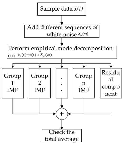
Figure 2.
EEMD flow chart.
4.2. Establishment of MPA-KELM Model
The regularization coefficient C and kernel function parameter σ are the key parameters that affect the performance of KELM neural network. In this paper, the MPA is used to optimize the regularization coefficient C and kernel function parameter σ in KELM, and the fault diagnosis model of tower dryer is established after obtaining the best parameters. The flow chart is shown in Figure 3.
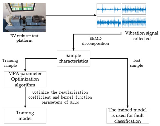
Figure 3.
RV Reducer fault diagnosis model based on MPA-KELM.
4.3. Evaluation Index
In order to comprehensively and effectively evaluate the performance of the proposed RV reducer fault diagnosis model based on EEMD-MPA-KELM, a multi-classification evaluation index system based on confusion matrix is selected in this paper, and the accuracy λA, accuracy λP, recall λR and Kappa coefficient are taken as the evaluation indexes of the RV reducer fault diagnosis model. The calculation formula is as follows:
In the formula, n represents the number of samples predicted correctly, N represents the total number of samples; nT represents the number of correctly predicted samples of a fault class, nR represents the total number of samples of this fault class, and nP represents the total number of samples predicted as this fault class. i = 1,2 indicates the two fault types of RV reducer.
Accuracy λA represents the comprehensive index of fault classification and prediction for tower dryer, and the higher the data is, the stronger the fault identification ability is. The accuracy λP represents the misjudgment index of a certain type of fault. The higher the accuracy, the higher the reliability of fault judgment. The recall ratio λR represents the missing judgment index of a certain type of fault. The higher the recall ratio, the higher the sensitivity of fault identification.
4.4. Model Performance Test
XJTU-SY bearing experimental data set was adopted for model test. In the test, sampling frequency was set as 25.6 kHz, sampling interval was 1 min, and each sampling duration was 1.28 s. The speed of the bearing is set at 2100 r/min, and the radial force received is 12 kN. Table 1 shows the fault forms of Bearing1_2, Bearing1_4, and Bearing1_5 in the data set.

Table 1.
Bearing data information.
The fault data were divided into 16 groups of sample data and decomposed by EEMD. The decomposed IMF is taken as input, and the classification number is taken as output. Classification 1 represents outer ring fault, classification 2 represents cage fault, classification 3 represents inner ring and outer ring fault, and classification 4 represents normal. The output is shown in the figure below.
It can be seen from Figure 4 that the prediction accuracy of the MPA-KELM model is much higher than that of the ELM model. As can be seen from Figure 5, the performance of the MPA-KIELM prediction model is still good, with fast running speed, small mean square error and good stability.
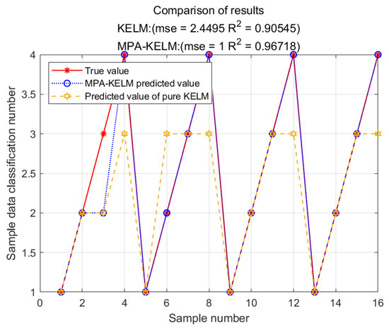
Figure 4.
Comparison of model prediction results.
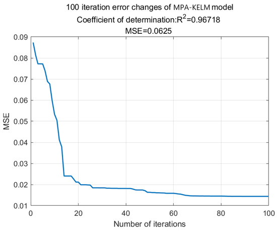
Figure 5.
Convergence diagram.
5. Test and Data Analysis
5.1. Test Platform
The specific model parameters of the RV reducer test platform used in the experiment are shown in Figure 6 and Table 2. the power of the servo motor is 5 kW, the measuring range of the torque sensor is 200 Nm, the measuring range of the torque sensor is 500 Nm, and the specification of the magnetic powder brake is 1.5 kW. The spindle speed is set to 151 r/min, and the input shaft and output shaft of the RV reducer are measured by the torque sensor. The RV reducer model number is RV-20E. Samples were collected at 0.5 s intervals and the experiment was conducted at normal temperature.
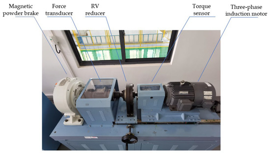
Figure 6.
RV reducer test platform.
Table 2.
Type parameters of RV reducer platform.
In the experiment, the torque, speed and power of the RV reducer appear abnormal data, and the reducer fails. Therefore, the data before the fault and the efficiency data after the fault are compared.
As can be seen from Figure 7, the efficiency before failure has certain periodicity, while the efficiency after failure is obviously not periodicity, which conforms to the conclusion of Equation (8).
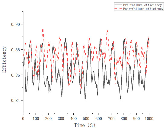
Figure 7.
Comparison before and after the fault.
5.2. Simulation of EEMD-MPA-KELM Fault Classification Model
MATLAB R2020b programming was used to select 1,680 monitoring data of pre-fault efficiency and post-fault efficiency as sample data for EEMD decomposition. Some graphs obtained are shown in Figure 8 and Figure 9.
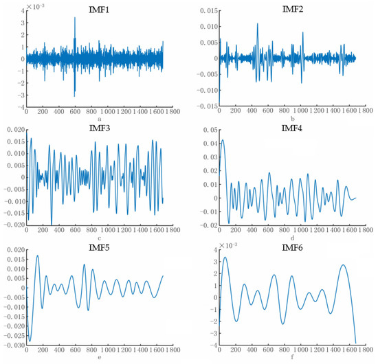
Figure 8.
IMF image after EEMD decomposition of normal data. (a) IMF1 component after EEMD decomposition of normal data; (b) IMF2 component after EEMD decomposition of normal data; (c) IMF3 component after EEMD decomposition of normal data; (d) IMF4 component after EEMD decomposition of normal data; (e) IMF5 component after EEMD decomposition of normal data; and (f) IMF6 component (residual component) after EEMD decomposition of normal data.
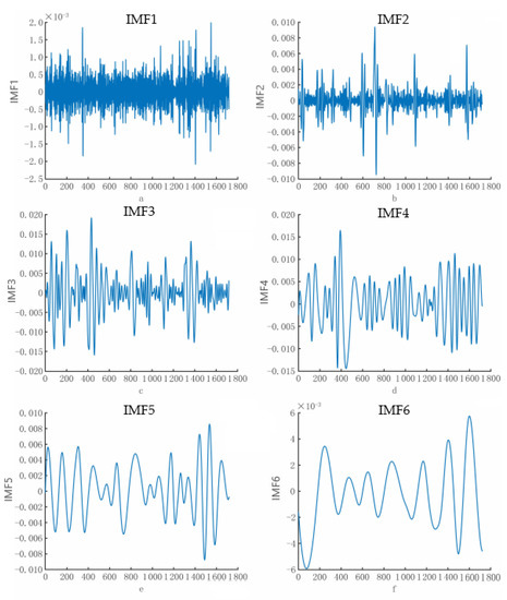
Figure 9.
Image of fault data after EEMD decomposition. (a) IMF1 component after EEMD decomposition of fault data; (b) IMF2 component after EEMD decomposition of fault data; (c) IMF3 component after EEMD decomposition of fault data; (d) IMF4 component after EEMD decomposition of fault data; (e) IMF5 component after EEMD decomposition of fault data; and (f) IMF6 component (residual component) after EEMD decomposition of fault data.
It can be seen from Figure 8 and Figure 9 that normal data and fault data are significantly different after EEMD decomposition. Since the energy of the signal is mainly concentrated in the lower IMF, the first six IMF components of each group are selected for average checking calculation. The two groups of data obtained 21 eigenvalues after collective average calculation. At this time, the eigenvalues were input into MPA-KELM classification model for training and classification. The decomposed IMF was taken as input, and the classification number was taken as output, among which classification 1 represented normal and classification 2 represented fault. The output is shown in Figure 10 and Figure 11.
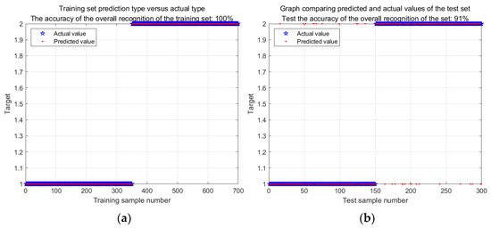
Figure 10.
Single operation result of EEMD-MPA-KELM model. (a) model training sets predict results; (b) model test sets predict results.
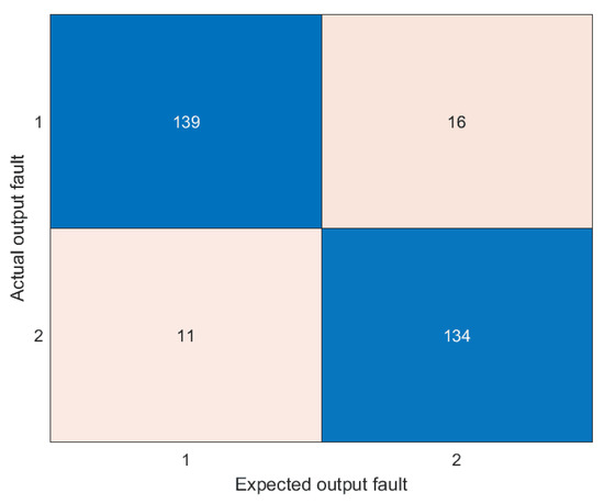
Figure 11.
Classification confusion matrix diagram of fault diagnosis.
It can be seen from Figure 10 that the EEMD-MPA-KELM diagnosis model has good recognition performance, and the overall recognition accuracy of its training set is relatively high, reaching 100%. The overall recognition accuracy of the test set is 90.33%.
Figure 11 shows the visual confusion matrix of RV reducer fault diagnosis results based on EEMD-MPA-KELM. The diagonal elements in the matrix represent the correct predicted number of samples of a certain fault class, and the sum of data in each column represents the total number of samples of this fault class, and the sum of data in each row represents the total number of samples predicted for this fault class. Table 3 shows the evaluation indexes of the model. It can be seen from Figure 10 and Table 3 that the recall and accuracy rates of the proposed EEMD-MPA-KELM fault diagnosis model for various samples of running state are both higher than 85%, and the diagnostic accuracy rate for cutting machine cut-off and tide discharge detection rod plugging is up to 100%. The Kappa coefficient of the model as a whole is 0.82. The Classification accuracy is as high as 91.00%. The proposed RV reducer fault diagnosis model based on EEMD-MPA-KELM is verified to have high fault recognition sensitivity, high fault judgment reliability and strong overall fault-classification ability.
Table 3.
Evaluation indexes of EEMD-MPA-KELM model.
In order to further verify the performance superiority of the proposed RV reducer fault diagnosis model based on EEMD-MPA-KELM, this model was compared and analyzed with the diagnostic results of other models. In order to eliminate the contingency of the test results, a total of 30 times were run, and the results are shown in Figure 12.
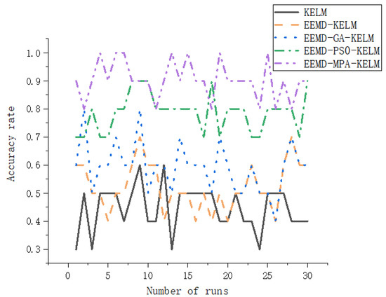
Figure 12.
Comparison of accuracy of 30 runs of various models.
As can be seen from Figure 12 and Table 4, the accuracy of KELM model is the lowest and unstable. The accuracy often fluctuates between 30–50%, and the overall accuracy is only 44.67%. After adding EEMD decomposition, the recognition accuracy of KEML was improved, and the overall accuracy was 52.33%. Although EEMD-GA-KELM model is relatively stable, its recognition accuracy is not much different from that of EEMD-KELM model, and its optimization effect is not obvious. The accuracy of EEMD-PSO-KELM model is relatively high, most of which is about 80%, and occasionally reaches 90%. EEMD-MPA-KELM model has the highest overall accuracy, with an average accuracy of 90.33% for 30 times, an overall accuracy of more than 90%, and even more than 100% for several times. The accuracy is relatively stable, and the optimization effect is the most significant.
Table 4.
Accuracy and running time statistics of each model after 30 runs.
In conclusion, the accuracy and stability of EEMD-MPA-KELM tower dryer fault diagnosis model are superior to the other four models.
6. Conclusions
The RV retarder is the core part of an industrial robot. With the increasing demand for industrial robot, it is very important to predict the failure of RV retarders in actual production. To solve the above problems, a fault diagnosis model of an RV reducer based on EEMD-MPA-KELM was proposed in this paper. After modeling and research, the following conclusions were obtained:
(1) The data measured on the RV reducer test platform is decomposed by EEMD to obtain the optimal special collection. The regularization coefficient C of KELM and the kernel function parameter σ are optimized with MPA to improve the prediction accuracy and stability of the KELM. The feature set is imported into the MPA-KELM model as input for fault identification. Compared with ELM, KEML, EEMD-GA-KELM and EEMD-PSO-KELM models, EEMD-MPA-KELM’s RV retarder fault diagnosis and classification model, this model is faster, more accurate and more stable.
(2) Timely and accurate judgment of the operation state of the RV reducer of industrial robots is conducive to the timely maintenance of the RV reducer, providing guarantee for the accuracy of the RV reducer test data, so as to help the RV reducer manufacturers to improve production efficiency and reduce economic losses.
Author Contributions
Conceptualization, Z.T.; Data curation, L.G.; Formal analysis, Y.L.; Funding acquisition, L.G. and Z.Z.; Investigation, Z.T.; Methodology, Z.T.; Project administration, Y.L.; Software, X.W.; Supervision, Y.L.; Validation, X.W. and Z.Z.; Visualization, Z.T.; Writing—review & editing, X.W.; Writing—original draft, X.W. and Z.T. All authors have read and agreed to the published version of the manuscript.
Funding
This research was funded by the Key research projects supported by the National Natural Science Foundation of China, grant number No. 92067205; Key Research and Development Project of Anhui Province, grant number No. 2022a05020035; Major science and technology project of Anhui Province, grant number No. 202103a05020022; HFIPS Director’s Fund, grant number No. YZJJQY202305; Supported by Anhui Province Intelligent Mine Technology and Equipment Engineering Laboratory Open Fund, grant number No. AIMTEEL202201; Key Project of Scientific Research of Anhui Provincial Education Department, China, grant number No. 2022AH050995.
Institutional Review Board Statement
Not applicable.
Informed Consent Statement
Not applicable.
Data Availability Statement
Not applicable.
Conflicts of Interest
The authors declare no conflict of interest.
References
- Pan, B.S.; Lin, C.K.; Xiang, Y.Y.; Wen, J.; Shi, L.J. Time-varying reliability analysis and optimal design of planetary Reducer transmission accuracy considering gear wear. Comput. Integr. Manuf. Syst. 2022, 28, 745–757. [Google Scholar]
- Li, Z.; Huang, X.L.; Zhang, T.F.; Jing, X. Fault diagnosis of Planetary Reducer based on multi-source heterogeneous sensor based on deep neural network. J. Ordnance Equip. Eng. 2018, 39, 192–195. [Google Scholar]
- Wang, J.G.; Ke, L.L. RV retarder fault diagnosis based on residual network. J. Mech. Eng. 2019, 55, 73–80. [Google Scholar] [CrossRef]
- Mao, J.; Guo, H.; Chen, H.Y. Fault diagnosis of shearer cutting gear based on deep self-coding network. Coal Sci. Technol. 2019, 47, 123–128. [Google Scholar]
- Peng, P.; Ke, L.L.; Wang, J.G. RV reducer fault diagnosis under noise interference. J. Mech. Eng. 2020, 56, 30–36. [Google Scholar] [CrossRef]
- Chen, L.R.; Cao, J.F.; Wang, X.Q. Fault diagnosis of RV reducer for robot based on nonlinear spectrum and kernel principal component analysis. J. Xi’an Jiaotong Univ. 2020, 54, 32–41. [Google Scholar]
- An, H.B.; Liang, W.; Zhang, Y.L. Analysis and Experimental study on Acoustic emission Signal Propagation Mechanism of Robot RV Reducer. Robot 2020, 42, 557–567. [Google Scholar]
- Yu, N.; Jing, N.; Chen, H.Y. Segmental fusion diagnosis method for compound fault of mine hoist retarder. Mech. Sci. Technol. 2022, 41, 394–401. [Google Scholar]
- Qian, H.-M.; Li, Y.-F.; Huang, H.-Z. Time-variant reliability analysis for industrial robot RV reducer under multiple failure modes using Kriging model. Reliab. Eng. Syst. Saf. 2020, 199, 106936. [Google Scholar] [CrossRef]
- Wang, H.; Jing, W.; Li, Y.; Yang, H. Fault Diagnosis of Fuel System Based on Improved Extreme Learning Machine. Neural Process. Lett. 2021, 53, 2553–2565. [Google Scholar] [CrossRef]
- Guo, S.; Wu, B.; Zhou, J.; Li, H.; Su, C.; Yuan, Y.; Xu, K. An Analog Circuit Fault Diagnosis Method Based on Circle Model and Extreme Learning Machine. Appl. Sci. 2020, 10, 2386. [Google Scholar] [CrossRef]
- Xia, Y.; Ding, Q.; Jiang, A.; Jing, N.; Zhou, W.; Wang, J. Incipient fault diagnosis for centrifugal chillers using kernel entropy component analysis and voting based extreme learning machine. Korean J. Chem. Eng. 2022, 39, 504–514. [Google Scholar] [CrossRef]
- Liu, X.; Huang, H.; Xiang, J. A personalized diagnosis method to detect faults in gears using numerical simulation and extreme learning machine. Knowl. Based Syst. 2020, 195, 105653. [Google Scholar] [CrossRef]
- Huang, G.-B. An Insight into Extreme Learning Machines: Random Neurons, Random Features and Kernels. Cogn. Comput. 2014, 6, 376–390. [Google Scholar] [CrossRef]
- Yang, X.; Yu, Z.D.; Zhang, Z.Y.; Bing, H.K.; Shen, H.N.; Wang, J.X. Turbine rotor fault diagnosis based on multi-feature extraction and nuclear extreme Learning machine. Turbine Technol. 2020, 62, 137–142. [Google Scholar]
- Qiao, W.S.; Hua, J.; Lou, R. Optimization of diesel engine fault diagnosis of nuclear Extreme Learning Machine with improved Butterfly algorithm. Mech. Des. Res. 2022, 38, 211–214. [Google Scholar]
- Liang, R.; Chen, Y.; Zhu, R. A novel fault diagnosis method based on the KELM optimized by whale optimization algorithm. Machines 2022, 10, 93. [Google Scholar] [CrossRef]
- Zhang, H.; Pan, C.; Wang, Y.; Xu, M.; Zhou, F.; Yang, X.; Zhu, L.; Zhao, C.; Song, Y.; Chen, H. Fault Diagnosis of Coal Mill Based on Kernel Extreme Learning Machine with Variational Model Feature Extraction. Energies 2022, 15, 5385. [Google Scholar] [CrossRef]
- Zhao, Z.; Ye, G.; Liu, Y.; Zhang, Z. Recognition of Fault State of RV Reducer Based on self-organizing feature map Neural Network. J. Physics Conf. Ser. 2021, 1986, 012086. [Google Scholar] [CrossRef]
- Mirjalili, S. Moth-flame optimization algorithm: A novel nature-inspired heuristic paradigm. Knowl. Based Syst. 2015, 89, 228–249. [Google Scholar] [CrossRef]
- Wu, Z.; Huang, N.E. Ensemble empirical mode decomposition: A noise-assisted data analysis method. Adv. Adapt. Data Anal. 2009, 1, 1–41. [Google Scholar] [CrossRef]
- Chen, J.M.; Liang, Z.C. Research on Speech Enhancement Algorithm based on EEMD Data preprocessing and DNN. J. Ordnance Equip. Eng. 2019, 40, 96–103. [Google Scholar]
- Wang, Y.J.; Kang, S.Q.; Zhang, Y.; Liu, X.; Jiang, Y.C. Condition Recognition Method of Rolling Bearing Based on Ensemble Empirical Mode Decomposition Sensitive Intrinsic Mode Function Selection Algorithm. J. Electron. Inf. Technol. 2014, 36, 595–600. [Google Scholar]


Disclaimer/Publisher’s Note: The statements, opinions and data contained in all publications are solely those of the individual author(s) and contributor(s) and not of MDPI and/or the editor(s). MDPI and/or the editor(s) disclaim responsibility for any injury to people or property resulting from any ideas, methods, instructions or products referred to in the content. |
© 2023 by the authors. Licensee MDPI, Basel, Switzerland. This article is an open access article distributed under the terms and conditions of the Creative Commons Attribution (CC BY) license (https://creativecommons.org/licenses/by/4.0/).