Article

Analysis of the Thermodynamic Characteristics of a Hyper-Compressor through Numerical Simulation and Experimental Investigation

School of Energy and Power Engineering, Xi’an Jiaotong University, Xi’an 710049, China
*
Author to whom correspondence should be addressed.
Appl. Sci. 2023, 13(7), 4478; https://doi.org/10.3390/app13074478
Submission received: 8 February 2023 / Revised: 16 March 2023 / Accepted: 29 March 2023 / Published: 31 March 2023

Abstract

:
Hyper-compressors play an important role in polymer production. However, due to the extremely high pressure and complex geometries, it is difficult to monitor and calculate the thermodynamic characteristics and pressure pulsation. In this research, a three-dimensional (3D) computational fluid dynamics (CFD) model of a hyper-compressor with a central valve and piston movements based on a real gas model (RGM) was developed to analyze the thermodynamic performance and pressure pulsation. Then, the p θ diagram of the working chamber and the dynamic pressure internal pipe were constructed using a nondestructive testing approach and showed a strong correlation with the pressure sensor data. The 3D-CFD model’s results correlated well with the experimental data. The deviation error between simulation values and experimental data of the indicated power was 1.77%. Lastly, the numerical model was used to analyze the hyper-compressor’s performance, power loss, dynamic features of the central valve and pressure pulsation.

1. Introduction

Low-density polyethylene (LDPE) is a thermoplastic derived from ethylene through polymerization. The technological flowchart consists of compression, polymerization, separation, and extrusion. First, ethylene has to be compressed at 20–30 MPa in a conventional reciprocating compressor (primary compressor), then at 100–350 MPa in a hyper-compressor system (secondary compressor) [1]. Given the flammable and explosive nature of ethylene and the extremely high pressures involved, the thermodynamic characteristics of the hyper-compressor and pressure pulsation of the thick-walled pipe must be paid special attention [2].
Various numerical methods, such as mathematic models [3], computational fluid dynamics (CFD) [4], and a finite element analysis (FEA) [5], are important tools for the design and analysis of the compressor components and piping system. First, the lumped-parameters method (LPM) is suited to the parametric study of the primary [6] and optimized [7] design of the key parameters. However, ignoring the effect of the pressure pulsation at the suction and discharge chamber leads to a large calculation error under ultra-high pressure [8]. Giacomelli Enzo [9] analyzed the pressure oscillations upstream and downstream of the cylinder’s impact on the hyper-compressor performance. However, the details of this method were not described. Second, a one-dimensional model based on acoustic wave theory and the transfer matrix was proposed to calculate the pressure pulsation [10]. Passeri Marco [11] used this method to evaluate the gas pulsation in a hyper-compressor system. Furthermore, it can also be used to estimate the attenuation effect of various pulsation attenuators [12,13]. However, this method is less accurate because it ignores the mutual effect of pressure changes in the working chamber and plant piping. Thus, Zhan Liu [14] proposed a hybrid method where the compressor was modeled based on the LPM and the pipeline was described using a gas dynamic model. This method can provide a better evaluation result of the compressor’s performance, but cannot reach convergence in cases of the resonant response of piping. Finally, Balduzzi Francesco [15] presented a 2D-CFD model of a reciprocating compressor to simulate the thermodynamic cycle, but the valves’ motion and pipes upstream and downstream of the compressor were ignored. Giacomelli Enzo [16] proposed 2D and 3D models of poppet valves for a hyper-compressor to evaluate the flow coefficient of valves, but did not consider the effect of pressure changes in the cylinder. Wu [17] built a whole dynamic model of a compressor with respect to the interaction between valve motion and pressure oscillations in the internal pipe to investigate the internal flow in the working chamber and the valve dynamic characteristics.
In addition, experimental investigation is another approach for the design of equipment and fault diagnosis. Multivariate physical state parameters have been used to monitor the operating status of the traditional reciprocating compressor, such as dynamic pressure [18], temperature [19], vibration [20], and valve lift [21]. However, most measurement methods inevitably need extraction holes to install various sensors. The flammable nature of ethylene and the extremely high-pressure working conditions mean that we cannot punch holes in the hyper-compressor and the plant pipe to avoid leakage. Thus, a nondestructive test method based on the theory of Roark’s formulas for stress and strain could be used for experimental investigation in hyper-compressors [22]. Transient pressure changes in the working chamber can be reconstructed by the piston load [23]. Pressure pulsation in the internal pipe could be obtained by measuring the axial and circumferential strain on the outside of the pipe [24]. However, this method was not validated with the pressure data directly measured by the pressure sensor.
In this research, a 3D-CFD model of a hyper-compressor and pipe system was built, considering the actual fluid properties under extremely high pressure and the interaction between valve motion and pressure pulsation. A real gas model (RGM) was utilized to improve the precision of the results. Suction and discharge pipelines were added to study the interaction between pressure fluctuations in the working chamber and pressure oscillations in the plant’s internal pipework. The method of nondestructive testing was presented to measure and recreate the p θ diagram and pressure pulsation, which was first validated using the pressure sensor’s recorded data. Experimental results were compared to the simulation results.

2. Numerical Calculation Model

To investigate the thermodynamic properties and pressure pulsation of the hyper-compressor, a 3D-CFD model incorporating valve and piston motion was established. Furthermore, the finite volume technique with a real gas model (RGM) was utilized.

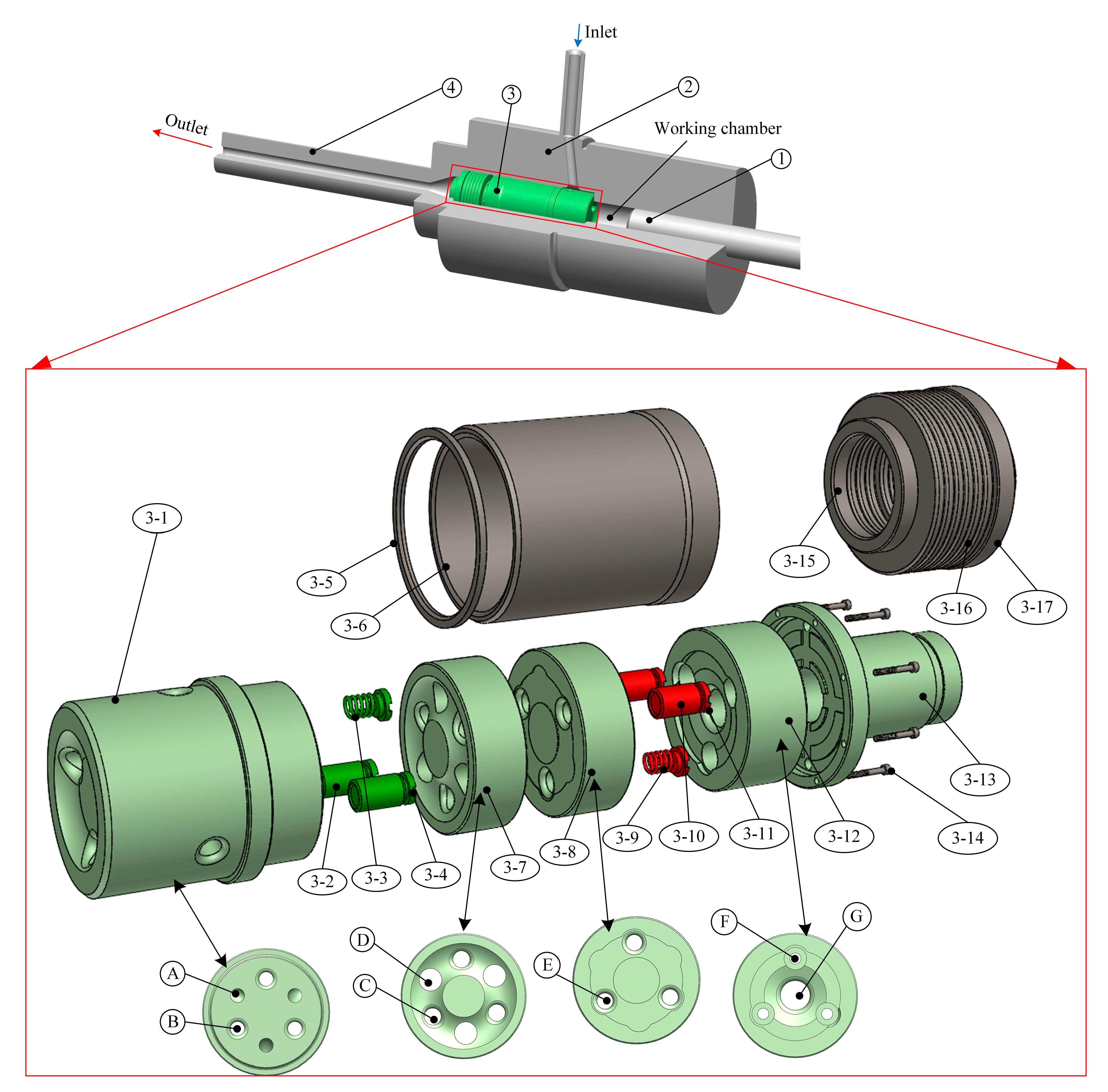
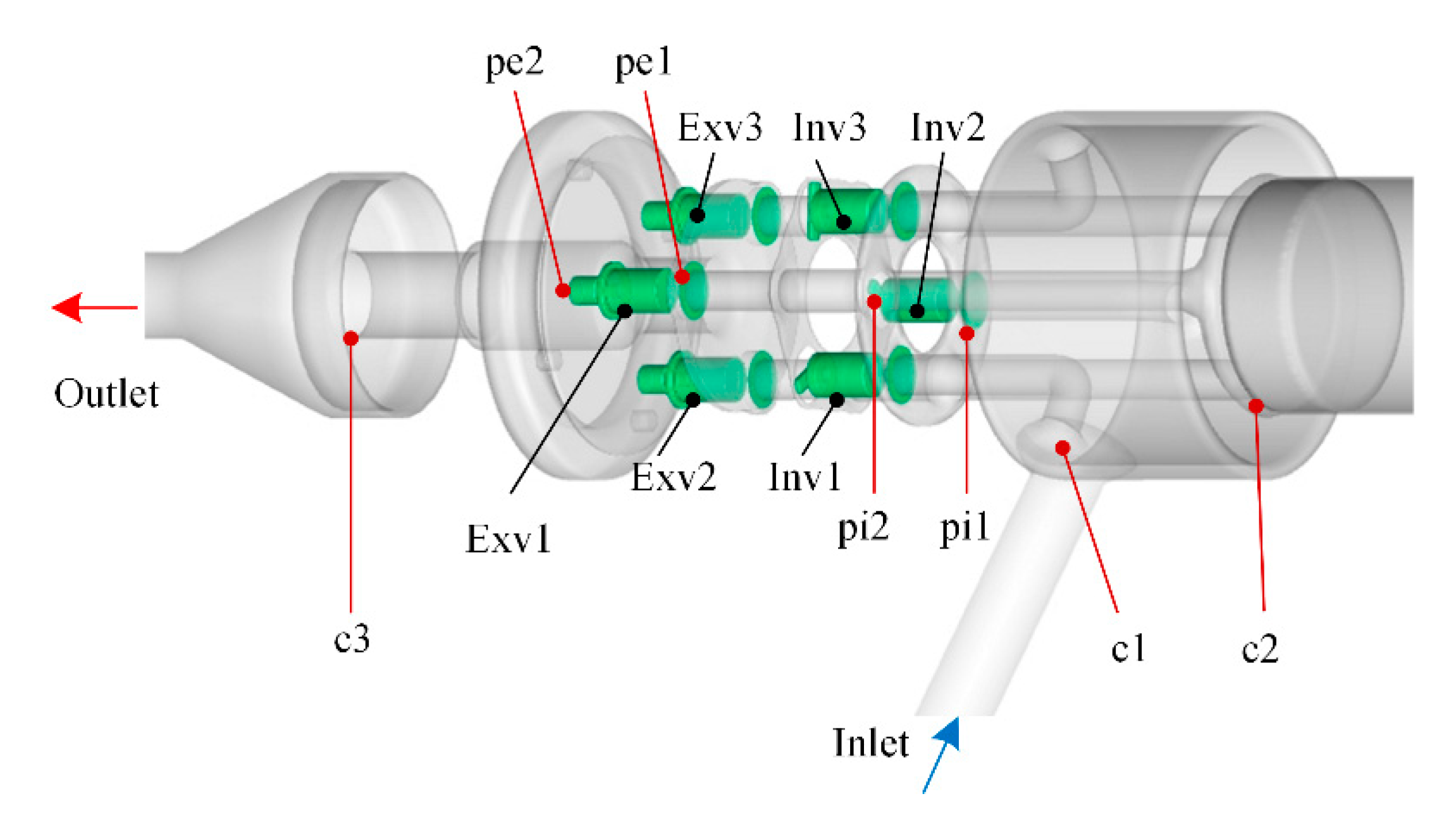
2.1. Physical and Numerical Model

The hyper-compressor is a plunger compressor (Figure 1). The central valve (3) is positioned within the spool’s hollow (2). Its axial sides are, respectively, connected to the working chamber and discharge pipe socket (4). Its circumferential side links through the spool (2) to the suc-pipe. The central valve (3) is a combination of suction and discharge multi-poppet valves for compact construction, which is composed of (3–1) a suction valve seat, (3–2) suction valve sleeves, (3–3) suc-springs, (3–4) suction spring seats, (3–5) a seal ring, (3–6) a guide sleeve, (3–7) a guide ring, (3–8) a middle piece, (3–9) dis-springs, (3–10) discharge valve sleeves, (3–11) discharge spring seats, (3–12) a discharge valve seat, (3–13) a discharge box, (3–14) screws, (3–15) a spring seat, (3–16) a combined disc spring, and (3–17) a gland nut.
The suction seat (3–1) is a cylinder with a number of radial through-holes (A and B) connecting it to the spool (2), a working chamber, and guide sleeve (3–7). A gap passage formed between the spool (2) and suction seat (3–1) serves as the gap from the suc-pipe passage through holes (A) to the concave side of the guide ring (3–7), and then into the working chamber through-holes (B). Simultaneously, almost no gas can flee through the clearance between the central valve (3) and the spool (2) because of the seal ring (3–5). The through-holes (B) in the suction seat (3–1), the holes (C) in the guide ring (3–7), and the holes (E) in the middle piece (3–8) are aligned along the same axis to form an internal passage between the cylinder and discharge valve seat (3–12), allowing the gas to flow from the working chamber to the concave side of the discharge valve seat (3–12) and then to the dis-pipe via the hole (G).
The suction and discharge valve (3–2/10) sleeves are the moving components of the central valve (3), which regulate the fluid flow direction. As illustrated in Figure 2, the discharge valve sleeves (3–10), spring seats (3–11), and springs (3–9) are installed in the holes (F) of the discharge valve seat (3–12) along the same axis. The discharge valve seat (3–12) directs the axial motion of the discharge valve sleeves (3–10), while the spring seats (3–11) limit their radial motion lift. For the exhaust process, the discharge valve sleeves (3–10) move to the spring seats (3–11) to connect the flow passage between the dis-pipe and the working chamber, or they are attached to the middle piece (3–7) to prevent gas leaking from the cylinder into the dis-pipe.
In addition, a small 0.05 mm gap is reserved to accommodate the generation of a new mesh during the valve sleeves’ opening phase. Simultaneously, the boundary between the gap and the flow domain of the middle piece (3–8) is either set as an interface to permit gas flow during the exhaust process, or as a wall to prevent gas leaks through the gap. The interface phase and wall events are calculated using LPM with RGM.
The structured mesh of the entire numerical model is shown in Figure 3. To reduce the effects of the numerical boundaries on the thermodynamic characteristics of the primary domain, the inlet and outlet boundaries were positioned before the suction buffer and reactor, respectively. The dynamic mesh update for the valve motion based on the force analysis could be expressed by the Equation (1).
M v x ¨ + C x ˙ + K x = F s + A v p d A v
where M v is the valve sleeve equivalent mass, K is the stiffness of the valve sleeve, x ¨ , x ˙ , and x are the acceleration, velocity, and lift of the valve sleeve, C is the damping coefficient, and F s is the spring force.

2.2. Numerical Methodology and Boundary Conditions

The time-dependent and Reynolds-averaged Navier–Stokes equations were used to solve the transient flow in the three-dimensional model [4]. The real gas model (RGM) was utilized (see Section 2.3) due to the extremely high pressure. The time-derivative terms were discretized by a second-order backward Euler scheme. The pressure–velocity coupling was solved by employing the pressure-implicit with splitting of operators (PISO).
The movement of the piston was updated at each time step based on Equation (2) [25]. The suction and discharge pressure and temperature (table in Section 3) with turbulence intensity of 5% were imposed as inlet and outlet boundary conditions (Figure 3). Considering that the 2–1A and 2–1B hyper-compressors share one intake buffer tank, and then the mutual effect of the pressure pulsation of 2–1A and 2–1B, the dynamic pressure and temperature monitored at the same position of 2–1B transformed 180° were loaded to the 2–1A as the boundary condition, to achieve both highly accurate results and to avoid unnecessary computational resources.
v = n π L 60 ( sin θ + λ 2 sin 2 θ 1 λ 2 sin 2 θ )
where v is the velocity of a piston, L is the stroke, and λ is the ratio of the crank radius to the connecting rod.
In addition, aiming to save on computational costs, the following assumptions were set:
  • Leakage was disregarded;
  • The heat exchange during the operating cycle was neglected;
  • The pressure pulsation in the piping in front of the inlet buffer tank was not considered.

2.3. Real Gas Model

The production of LDPE by the kettle method needs to compress ethylene to 180–260 Mpa through several stages of compressors. According to Nowak [26], the critical parameters of ethylene are as follows: p c r = 5.0418   Mpa ; T c r = 282.35   K .
Evidently, ethylene is in a supercritical state in this case ( p / p c r > > 1 ; T / T c r > > 1 ), and the intermolecular forces cannot be neglected. The ideal gas equation of the state is therefore no longer applicable. A real gas model (RGM) should be proposed to provide a more accurate depiction of the fluid behavior.
An RGM implements the equation of the state in an explicit form in the Helmholtz energy [27] for the thermodynamic properties. The Helmholtz energy ( α = a / ( R T ) ) can be written as:
α ( δ , τ ) = α o ( δ , τ ) + α r ( δ , τ )
where δ = ρ / ρ c r ; τ = T c r / T , while α o and α r are the ideal and residual parts of the Helmholtz energy, respectively.
The process of calculating thermodynamic and transport properties using the Helmholtz energy is depicted in Figure 4.
Furthermore, viscosity and thermal conductivity are modeled with empirical functions [28,29,30].

2.4. Mesh Independence Check

A mesh independence check must be conducted to assess the suitable mesh density for achieving highly precise results while minimizing computational resources. The numerical model (Figure 3) was rebuilt with three structured mesh levels, and the simulation results for the mass flow rate and indicated power are presented in Table 1. Clearly, the difference in the indicated power and mass flow between tests 2 and 3 was less than 0.1%. The mesh of item 2 was then utilized.

3. Experimental Verification

An experimental study has to be performed to validate the numerical model before the simulation results can be used to analyze the thermodynamic characteristics of the hyper-compressor.
As shown in Figure 5 and Table 2, a two-stage, eight-cylinder, opposed-balanced, four-row, large-scale hyper-compressor system was modified for the test. The hyper-compressor was equipped with a data acquisition system along with several sensors that recorded the signals of the piston rod, pipe strain, and piston position. Then, these signals were reconstructed based on the non-destructive test method (NDT) to obtain the p θ diagram and pipe dynamic pressure.

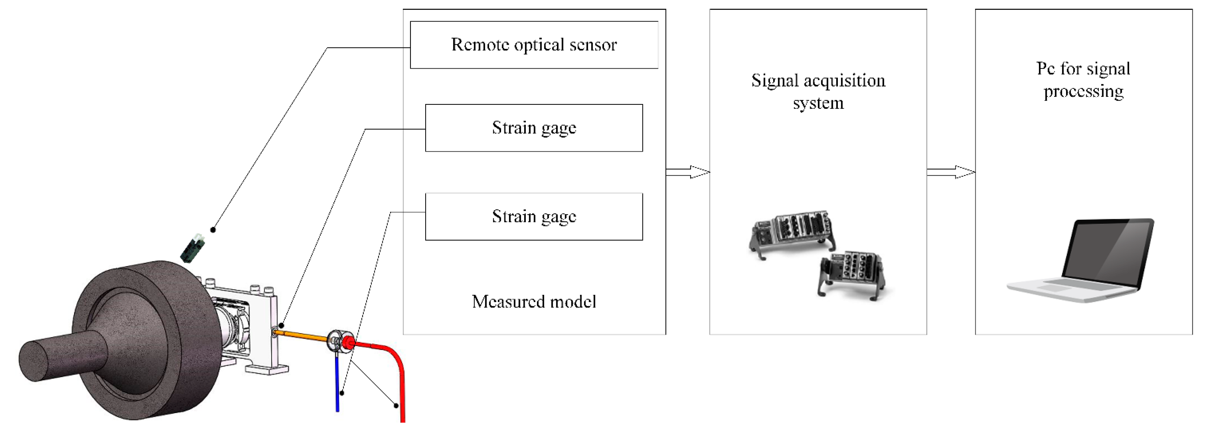
3.1. Measurement of the TDC Signal

In order to determine the crank angle, a remote optical sensor was installed at the compressor frame, which generated a pulse signal as the piston arrived at the TDC (top dead center) during each operating cycle. Thus, the crank angle was set to 0° at this time and the operating time was converted to the crank angle for Section 3.2 and Section 3.3.

3.2. Measurement and Construction of the p θ Diagram

The thickness components and safety devices in case of leakage around the cylinder do not permit the installation of a pressure sensor measuring the dynamic pressure in the cylinder. The non-destructive test (NDT) based on the force-induced strain on the piston was used to measure and construct the p θ diagram. The pressure in the working chamber equals F g divided by A p , and then F g can be reconstructed based on the main acting forces analysis in the piston (Equation (4)).
F g = F p F r i F f
The reciprocating inertial force F r i and friction force F f can be obtained with known variables (Equations (5) and (6)). The piston rod load F p has only one independent unknown variable: stress σ on the piston, which can be obtained from the measured strain (Equation (7)).
F r i = M s r ω 2 cos θ + λ M s r ω 2 cos 2 θ
F f = κ ( M s g F p λ 1 λ 2 sin 2 θ )
F p = π D p 2 4 σ u p + σ d o w n 2
where M s is the reciprocating inertial mass and κ is the dynamic friction coefficient.
Considering the factors of temperature, gravity, and extremely high pressure, two two-axis 90-degree angle strain gages were installed in diametrically opposite positions to measure the axial and circumferential strain, which had a quarter bridge with temperature compensation.

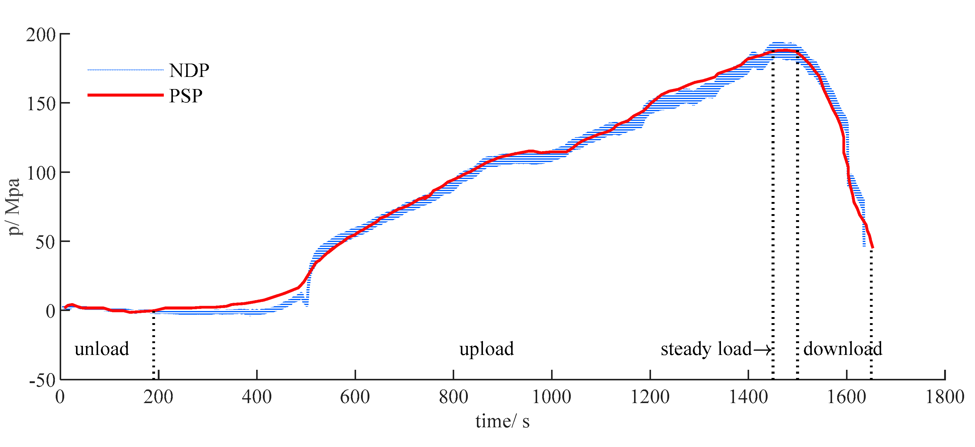
3.3. Measurement and Reconstruction of the Pressure Pulsation in the Pipe

The dynamic pressure in the pipeline can be calculated by the stress on the pipe’s surface tension [31], based on the pressure vessel theory [22].
σ c = 2 σ a = p 2 D int 2 D e x t 2 D int 2
where σ c and σ a are the circumferential and axial strains, respectively.
According to Hooke’s law for linearly elastic isotropic materials, the inner pressure can be calculated by the measured strain using the following functions:
σ a = E 1 υ 2 ( ε a + υ ε c ) σ c = E 1 υ 2 ( ε c + υ ε a )
where E is Young’s modulus, ε c and ε a are the circumferential and axial stress, respectively, υ is Poisson’s ratio,
Combining Equations (8) and (9), the internal dynamic pressure can be reconstructed by the axial and circumferential strains measured by the strain gauges.
p = D e x t 2 D int 2 2 D int 2 E 1 υ 2 ( ε c + υ ε a )

3.4. Validation of the NDT

In order to verify the accuracy of the NDT, a strain gauge was attached near the pressure sensor installed at the stage of pipe fabrication. The reconstructed pressure based on the NDT (Section 3.2) and the pressure measured by a pressure sensor (PSP) were compared during the entire test run (Figure 6). The pressure change based on the NDT was in good agreement with the PSP, particularly during the steady load process, with the exception of the initial upload time. The deviation during the initial upload process can be explained by the strain gauge’s inability to distinguish the stress caused by the minute but sudden changes in the internal pressure. However, as the working pressure was increasing gradually and the stress fluctuation could be negligible, the deviation had very limited effects.
Correspondingly, the results indicate that the NDT was valid and the pressure reconstructed by the strain on the outside of the pipe could be used to analyze the pressure pulsation of the hyper-compressor system.

4. Discussion

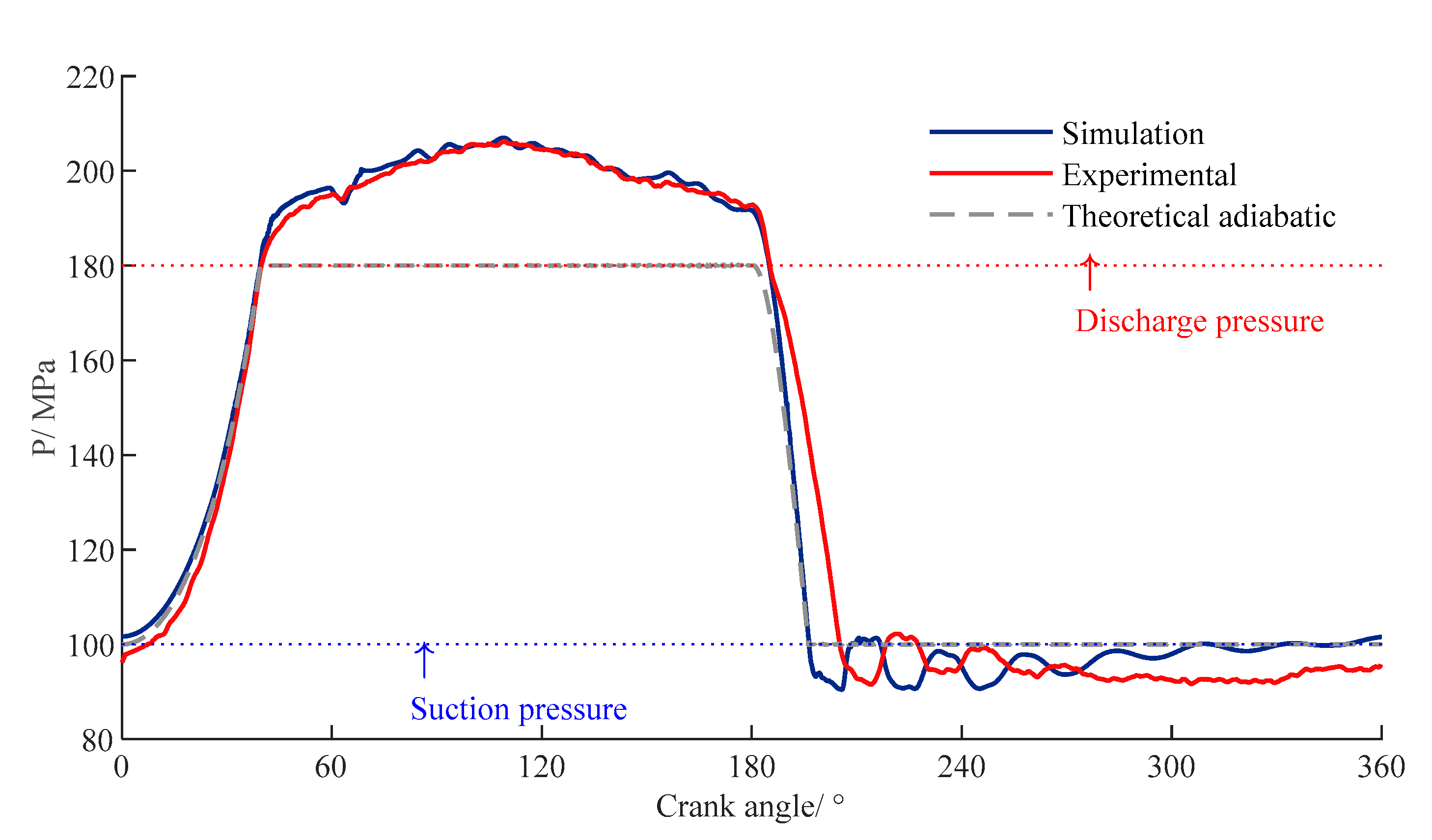
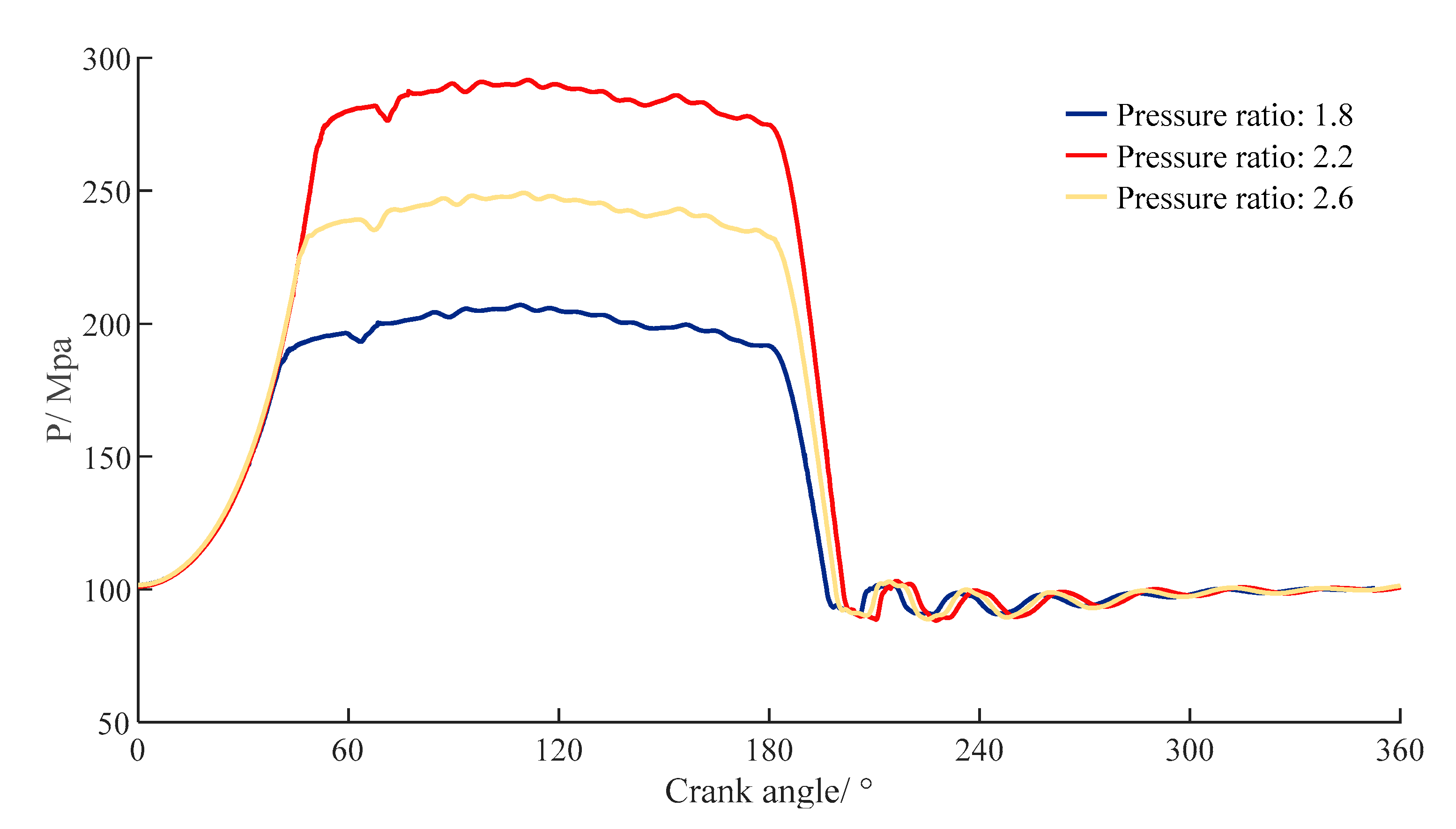
4.1. Dynamic Pressure in the Working Chamber

Figure 7 depicts the p θ diagram inside the working chamber of the numerical and experimental results. The numerical model’s predicted p θ diagram was in good agreement with the experimental data. Pressure changes during the compression and discharge phases of the numerical results and experimental values followed a nearly identical trend. The worst prediction by the numerical model appeared in the expansion and suction process, and the pressure difference between the simulated values and experimental data gradually increased with the increase in the crank angle. The indicated power of the simulation and experiment was 547.85 kW and 557.73 kW, respectively, demonstrating a small deviation error. The estimated discharge power loss was 108.33 kW, which deviated from the experimental value (100.70 kW) by 7.58%.
The deviation could be explained by the simulation model’s failure to account for leakage and its simplification of the 1–2A hyper-compressor’s effect. Furthermore, ethylene would polymerize under extremely high pressure, and the micro polymers would adhere to the inner walls. In the computational model, the effectiveness of these micro polymers was not considered. In addition, the numerical model did not account for heat transfer, which had an impact on the actual working cycle due to the low compressor speed. Finally, the deviation of nondestructive testing cannot be neglected.
The pressure ratio in this experimental test was 1.8. However, the maximum could reach 2.6. Therefore, the numerical model was used to study the dynamic features of the hyper-compressor system under three operating situations (pressure ratio: 1.8, 2.2, 2.6). Figure 8 and Table 3 depict the p θ diagram and power consumption for various pressure ratios, respectively. It can be seen that there was a roughly linear positive correlation between the discharge loss and the pressure ratio. Additionally, the different exhaust pressures had little impact on the suction process, because the central valve isolated the impact of the exhaust pipe on the dynamic pressure inside the working chamber during the suction process.

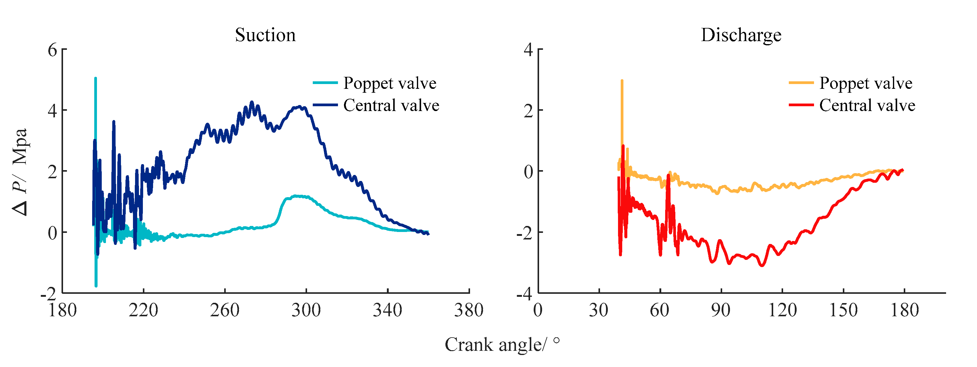
4.2. The Performance of the Central Valve

In contrast to the ring or mesh valve installed in the primary reciprocating compressor, the central valve installed in the hyper-compressor combines the suction and discharge multi-poppet valves and has a complex geometric structure. In order to analyze the valve movement, power loss, and other features of the central valve, the simulation especially monitored the various parameters at numerous important sites (Figure 9).

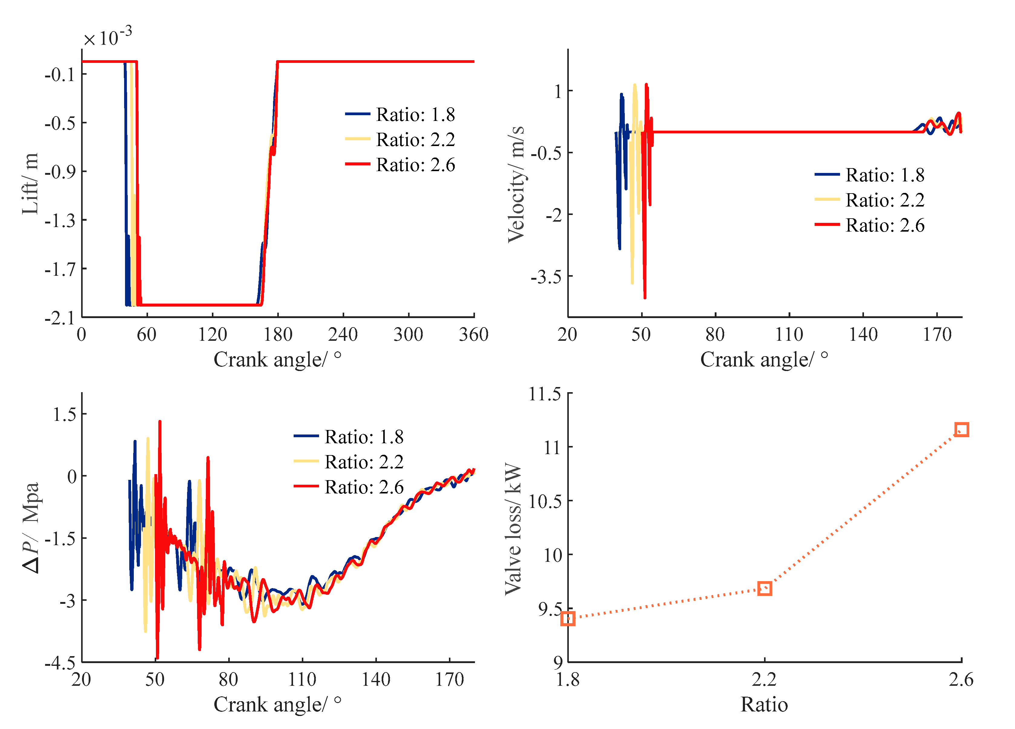
4.2.1. Poppet Valve Motion

Figure 10 depicts the lift of the suction/discharge poppet valves. For the suction poppet valves, Inv1 (Figure 9), which is closest to the inlet, has a significantly larger gas force than Inv2 and Inv3. The gas force matched the spring force appropriately, and the opening and closing process took the least amount of time and remained fully open for the longest period of time with a good motion pattern; In3 (Figure 9), which is the farthest from the inlet, had the lowest gas force and obvious chattering after the valve sleeve was just opened, and it repeatedly hit the spring seat.

4.2.2. Valve Power Loss

In order to study the effect of the complex geometry of the central valve, the movement law of the poppet valve, the lift, and the effective flow area on the valve loss, the pressure drop of the fluid through the center valve (c1-c2/c2-c3), and the poppet valve (pi1-pi2/pe1-pe2) for the suction and exhaust processes was monitored (Figure 9). According to Figure 11 and Table 4, the valve loss was produced mostly by the complex geometric structure of the central valve, while the structure and movement of the poppet valve had little impact on the power loss. From Figure 9, it is clear that the fluid during the suction process would pass through multiple 90-degree bends, while the fluid during the exhaust process would pass through no bends except at the poppet valves. This was the primary reason why the central valve loss of the suction process was greater than that of the exhaust process.

4.2.3. Effect of the Pressure Ratio

Figure 12 illustrates the lift (top-left) and velocity (top-right) of Exv2, as well as the pressure drop (bottom-left) and valve loss (bottom-right) of the central valve during the exhaust process at various pressure ratios. The greater the pressure ratio, the quicker the valve opens, and the faster the valve sleeve hits the spring seat, the shorter the valve’s lifespan. In addition, the overall trend of the pressure drop was unrelated to the pressure ratio, but roughly the same as the piston motion (Equation (2)) trend, which first increased and then decreased. Furthermore, the larger the pressure ratio, the greater the pressure drop in the valve opening’s early peak, and the greater the valve loss.

4.3. The Effect of the Dis-Pipe Pressure Pulsation

The dynamic pressure of the internal discharge pipe near the hyper-compressor (Figure 5) was monitored in the test and simulation simultaneously. As shown in Figure 13, the pressure changes with the crank angle showed similar overall trends between the numerical results and experimental data. There was one large pressure wave during the exhaust process, then the pressure was slowly decreased with the crank angle. The estimated pressure irregularity ( 100 ( p max p min ) / p 0 ) was 11.70%, which deviated from the experimental value (12.58%) by 7.01%. The first and second orders of amplitude with the simulation results and experimental data had relative deviations of 7.91% and 6.66%, respectively.
The pressure fluctuations in the dis-pipe can be attributed to the hyper-compressor’s periodic exhaust. In addition, adding 4.1 and 4.2 reveals that the valve loss accounted for just 9.60% of the discharge power loss, while the remaining power loss was mainly caused by the pressure pulsation. As shown in Figure 13, there was a large wave during the discharge process, as no pulsation attenuator was installed in the discharge pipeline.

5. Conclusions

A few conclusions based on the experimental and simulated study of the hyper-compressor in this work can be summarized as follows:
  • A non-destructive method based on material stress was proposed to measure and construct a p θ diagram of a hyper-compressor and the pressure of an internal pipe, which demonstrated good agreement with the directly measured pressure;
  • The 3D-CFD model considering piston and valve motions could predict the thermodynamic performance and pressure pulsation of the hyper-compressor with reasonable precision compared to the experimental results;
  • The RGM was of great importance for the simulated results;
  • The valve loss was produced primarily by the complex geometric structure, while the structure and movement of the poppet valve had little impact on the power loss;
  • The poppet valve closest to the inlet was fastest-closing and the valve farthest from the inlet had obvious flutter;
  • The valve loss represented a small amount of power loss in an operating cycle, and the major power loss was due to pressure pulsation in the discharge process;
  • A pulsation attenuator should be installed in both the suction and discharge pipe near the hyper-compressor.

Author Contributions

Conceptualization, X.J. and L.Y.; methodology, L.Y.; software, L.Y.; validation, X.J. and L.Y.; formal analysis, L.Y.; investigation, L.Y.; resources, X.J.; data curation, L.Y.; writing—original draft preparation, L.Y.; writing—review and editing and X.P. and X.J.; visualization, L.Y.; supervision, X.P.; project administration, L.Y.; funding acquisition, X.P. All authors have read and agreed to the published version of the manuscript.

Funding

This research was funded by the National Natural Science Foundation of China, Grant number 52076166.

Institutional Review Board Statement

This study did not involve humans or animals.

Informed Consent Statement

This study did not involve humans or animals.

Data Availability Statement

This study did not report any data.

Conflicts of Interest

The authors declare no conflict of interest. The funders had no role in the design of the study; in the collection, analyses, or interpretation of the data; in the writing of the manuscript, or in the decision to publish the results.

Nomenclature

Notation
M v Valve sleeve equivalent mass
K Stiffness of valve spring
x ¨ Acceleration of valve sleeve
x ˙
x
Velocity of valve sleeve
Displacement of valve sleeve
C Damping coefficient
F Force
p Pressure
A v Area of valve
v velocity
L Stroke
n Rotational speed
R
a
Molar gas constant
Specific Helmholtz energy
T Temperature
c p Isobaric heat capacity
c v
B
C
h
u
w
s
P O W
m
Isochoric heat capacity
Second viral coefficient
Third viral coefficient
Specific enthalpy
Specific internal energy
Speed of sound
Specific entropy
Indicated power
Mass flow rate
g Gravitational acceleration
M s Reciprocating inertial mass
r Crank radius
E Young’s modulus
D Diameter
Greek letters
λ Ratio of crank radius to connecting rod
θ Crank angle
α Dimensionless Helmholtz energy
δ Reduced density
τ Inverse reduced temperature
ρ Density
Δ Difference
κ Dynamic friction coefficient
σ Stress
ω Angular velocity of crankshaft rotation
ε Strain
υ Poisson’s ratio
Subscripts
p Piston rod
c r At the critical point
s Suction
d Discharge
f Friction
g Gas
r i
int
e x t
Reciprocating inertia
Internal
External
c Circumferential
a Axial
Superscripts
o Ideal gas part
r Residual part
Saturated liquid state
Saturated vapor state

References

  1. Giacomelli, E.; Battagli, P.; Lumachi, F.; Gimignani, L. Safety Aspects of Design of Cylinders and Hyper-Compressors for LDPE; ASME: San Diego, CA, USA, 2004. [Google Scholar]
  2. Passeri, M.; Generosi, S.; Bagagli, R.; Maggi, C. Preliminary Piping Sizing and Pressure Pulsation Evaluation; ASME: Anaheim, CA, USA, 2014. [Google Scholar]
  3. Tuhovcak, J.; Hejcik, J.; Jicha, M. Comparison of Heat Transfer Models for Reciprocating Compressor. Appl. Therm. Eng. 2016, 103, 607–615. [Google Scholar] [CrossRef]
  4. Anderson, J.D.; Wendt, J. Computational Fluid Dynamics; Springer: New York, NY, USA; McGraw-Hill: New York, NY, USA, 1995; Volume 206, ISBN 978–3-540-85055-7. [Google Scholar]
  5. Bhavikatti, S.S. Finite Element Analysis; New Age International: New Delhi, India, 2005; ISBN 81-224-1589-X. [Google Scholar]
  6. Costagliola, M. The Theory of Spring-Loaded Valves for Reciprocating Compressors. J. Appl. Mech. 1950, 17, 415–420. [Google Scholar] [CrossRef]
  7. Sun, X.; Wang, Y.; Zhang, J.; Lei, F.; Zhao, D.; Hong, H. Multi-Objective Optimization Design of Key Parameters of a Stepless Flow Control System with Multi-System Coupling Characteristics. Appl. Sci. 2022, 12, 1301. [Google Scholar] [CrossRef]
  8. Mohammadi-Amin, M.; Jahangiri, A.R.; Bustanchy, M. Thermodynamic Modeling, CFD Analysis and Parametric Study of a near-Isothermal Reciprocating Compressor. Therm. Sci. Eng. Prog. 2020, 19, 100624. [Google Scholar] [CrossRef]
  9. Giacomelli, E.; Shi, J.-X.; Manfrone, F. Considerations on Design, Operation and Performance of Hypercompressors; American Society of Mechanical Engineers Digital Collection: Bellevue, DC, USA, 2010; pp. 31–40. [Google Scholar]
  10. Grover, S.S. Analysis of Pressure Pulsations in Reciprocating Compressor Piping Systems. J. Eng. Ind. 1966, 88, 164–168. [Google Scholar] [CrossRef]
  11. Giacomelli, E.; Passeri, M.; Zagli, F.; Generosi, S. Control of Pulsations and Vibrations in Hypercompressors for LDPE Plants; American Society of Mechanical Engineers Digital Collection: San Diego, CA, USA, 2004; Volume 46687, pp. 73–79. [Google Scholar]
  12. Liu, B.; Feng, J.; Wang, Z.; Peng, X. Attenuation of Gas Pulsation in a Reciprocating Compressor Piping System by Using a Volume-Choke-Volume Filter. J. Vib. Acoust. 2012, 134, 051002. [Google Scholar] [CrossRef]
  13. Mlynarczyk, P.; Cyklis, P. The Estimation of the Pressure Pulsation Damping Coefficient of a Nozzle. J. Sound Vib. 2020, 464, 115002. [Google Scholar] [CrossRef]
  14. Liu, Z.; Jia, W.; Liang, L.; Duan, Z. Analysis of Pressure Pulsation Influence on Compressed Natural Gas (CNG) Compressor Performance for Ideal and Real Gas Models. Appl. Sci. 2019, 9, 946. [Google Scholar] [CrossRef] [Green Version]
  15. Balduzzi, F.; Tanganelli, A.; Ferrara, G.; Babbini, A. Two-Dimensional Approach for the Numerical Simulation of Large Bore Reciprocating Compressors Thermodynamic Cycle. Appl. Therm. Eng. 2018, 129, 490–501. [Google Scholar] [CrossRef]
  16. Giacomelli, E.; Schiavone, M.; Manfrone, F.; Raggi, A. Flow Coefficient Evaluation of Poppet Valves Used in Reciprocating Compressors for LDPE; American Society of Mechanical Engineers Digital Collection: Chicago, IL, USA, 2008; Volume 5, pp. 123–129. [Google Scholar]
  17. Wu, W.; Guo, T.; Peng, C.; Li, X.; Li, X.; Zhang, Z.; Xu, L.; He, Z. FSI Simulation of the Suction Valve on the Piston for Reciprocating Compressors. Int. J. Refrig. 2022, 137, 14–21. [Google Scholar] [CrossRef]
  18. Sun, X.; Zhang, J.; Wang, Y.; Wang, J.; Qi, Z. Optimization of Capacity Control of Reciprocating Compressor Using Multi-System Coupling Model. Appl. Therm. Eng. 2021, 195, 117175. [Google Scholar] [CrossRef]
  19. Townsend, J.; Badar, M.A.; Szekerces, J. Updating Temperature Monitoring on Reciprocating Compressor Connecting Rods to Improve Reliability. Eng. Sci. Technol. Int. J. 2016, 19, 566–573. [Google Scholar] [CrossRef] [Green Version]
  20. Cerrada, M.; Macancela, J.-C.; Cabrera, D.; Estupiñan, E.; Sánchez, R.-V.; Medina, R. Reciprocating Compressor Multi-Fault Classification Using Symbolic Dynamics and Complex Correlation Measure. Appl. Sci. 2020, 10, 2512. [Google Scholar] [CrossRef] [Green Version]
  21. Zhao, B.; Jia, X.; Sun, S.; Wen, J.; Peng, X. FSI Model of Valve Motion and Pressure Pulsation for Investigating Thermodynamic Process and Internal Flow inside a Reciprocating Compressor. Appl. Therm. Eng. 2018, 131, 998–1007. [Google Scholar] [CrossRef]
  22. Young, W.C.; Budynas, R.G.; Sadegh, A.M. Roark’s Formulas for Stress and Strain, 8th ed.; The McGraw-Hill Companies, Inc.: New York, NY, USA, 2012. [Google Scholar]
  23. Li, X.; Peng, X.; Zhang, Z.; Jia, X.; Wang, Z. A New Method for Nondestructive Fault Diagnosis of Reciprocating Compressor by Means of Strain-Based p–V Diagram. Mech. Syst. Signal Process. 2019, 133, 106268. [Google Scholar] [CrossRef]
  24. Carcasci, C.; Sacco, M.; Landucci, M.; Fiaschi, M. From Piping Deformation to Pressure Pulsation Measurements to Solve LDPE Plants Vibration Issues; American Society of Mechanical Engineers Digital Collection: Prague, Czech Republic, 2018; Volume 5. [Google Scholar]
  25. Sun, S.-Y.; Ren, T.-R. New Method of Thermodynamic Computation for a Reciprocating Compressor: Computer Simulation of Working Process. Int. J. Mech. Sci. 1995, 37, 343–353. [Google Scholar] [CrossRef]
  26. Nowak, P.; Kleinrahm, R.; Wagner, W. Measurement and Correlation of the (p, ρ,T) Relation of Ethylene II. Saturated-Liquid and Saturated-Vapour Densities and Vapour Pressures along the Entire Coexistence Curve. J. Chem. Thermodyn. 1996, 28, 1441–1460. [Google Scholar] [CrossRef]
  27. Smukala, J.; Span, R.; Wagner, W. New Equation of State for Ethylene Covering the Fluid Region for Temperatures From the Melting Line to 450 K at Pressures up to 300 MPa. J. Phys. Chem. Ref. Data 2000, 29, 1053–1121. [Google Scholar] [CrossRef]
  28. Holland, P.M.; Eaton, B.E.; Hanley, H.J.M. A Correlation of the Viscosity and Thermal Conductivity Data of Gaseous and Liquid Ethylene. J. Phys. Chem. Ref. Data 1983, 12, 917–932. [Google Scholar] [CrossRef]
  29. Klein, S.A.; McLinden, M.O.; Laesecke, A. An Improved Extended Corresponding States Method for Estimation of Viscosity of Pure Refrigerants and Mixtures. Int. J. Refrig. 1997, 20, 208–217. [Google Scholar] [CrossRef]
  30. Assael, M.J.; Koutian, A.; Huber, M.L.; Perkins, R.A. Reference Correlations of the Thermal Conductivity of Ethene and Propene. J. Phys. Chem. Ref. Data 2016, 45, 033104. [Google Scholar] [CrossRef] [PubMed]
  31. Fusi, A.; Cappelli, L.; Carcasci, C.; Sacco, M. Tuning of the Acoustical Analysis Model for Hypercompressors through Strain Gage Pulsation Measurements; American Society of Mechanical Engineers Digital Collection: San Antonio, TX, USA, 2019; Volume 5. [Google Scholar]
Figure 1. Schematic view of the hyper-compressor and central valve.
Applsci 13 04478 g001
Figure 2. The flow domain of the hyper-compressor.
Applsci 13 04478 g002
Figure 3. Mesh of the entire flow domain.
Applsci 13 04478 g003
Figure 4. Program flowchart of the Helmholtz energy.
Applsci 13 04478 g004
Figure 5. Schematic of the hyper-compressor test system.
Applsci 13 04478 g005
Figure 6. Comparison of the reconstructed pressure with the measured pressure.
Applsci 13 04478 g006
Figure 7. Diagram inside the working chamber.
Applsci 13 04478 g007
Figure 8. Diagram inside for different pressure ratios.
Applsci 13 04478 g008
Figure 9. Central valve fluid domain and monitoring sites.
Applsci 13 04478 g009
Figure 10. Suction (left) and discharge (right) poppet valve lift.
Applsci 13 04478 g010
Figure 11. The pressure drop of the suction (left) and discharge (right) process.
Applsci 13 04478 g011
Figure 12. Valve performance for various pressure ratios during the discharge process.
Applsci 13 04478 g012
Figure 13. Pressure pulsation (left) and amplitude–frequency (right) in the dis-pipe near the compressor.
Applsci 13 04478 g013
Table 1. Mesh convergency study of the mesh level.
Item12(Ref)3
No of mesh /1061.271.732.05
P O W / P O W r e f 0.984411.00045
m / m r e f 0.981711.0034
Table 2. Specifications of the hyper-compressor system.
ParametersUnit
Crank radiusmm170
Connecting rod length mm800
Speed rpm200
Piston diameter mm80
Clearance volume%31
Substance-Ethylene
Suction/discharge pressure MPa100/180
Suction/discharge temperature K294/317
Table 3. Indicated power and power loss.
Pressure Ratio1.82.22.6
Indicated power/kW557.73763.14960.78
Suction loss/kW20.0921.0420.35
Discharge loss/kW108.33116.66124.10
Table 4. Valve loss.
Valve Power Loss/kWPoppet ValveCentral Valve
Suction1.2314.50
Discharge2.0710.43
Disclaimer/Publisher’s Note: The statements, opinions and data contained in all publications are solely those of the individual author(s) and contributor(s) and not of MDPI and/or the editor(s). MDPI and/or the editor(s) disclaim responsibility for any injury to people or property resulting from any ideas, methods, instructions or products referred to in the content.

