Modeling a Typical Non-Uniform Deformation of Materials Using Physics-Informed Deep Learning: Applications to Forward and Inverse Problems

Abstract

Numerical methods, such as finite element or finite difference, have been widely used in the past decades for modeling solid mechanics problems by solving partial differential equations (PDEs). Differently from the traditional computational paradigm employed in numerical methods, physics-informed deep learning approximates the physics domains using a neural network and embeds physics laws to regularize the network. In this work, a physics-informed neural network (PINN) is extended for application to linear elasticity problems that arise in modeling non-uniform deformation for a typical open-holed plate specimen. The main focus will be on investigating the performance of a conventional PINN approach to modeling non-uniform deformation with high stress concentration in relation to solid mechanics involving forward and inverse problems. Compared to the conventional finite element method, our results show the promise of using PINN in modeling the non-uniform deformation of materials with the occurrence of both forward and inverse problems.

1. Introduction

The non-uniform deformation of solid materials, and in particular the strong non-uniform deformation caused by the concentration of stress at the boundary, is an extremely important issue in stress analysis, material processing, mechanical manufacturing, etc. Modeling the non-uniform deformation of solid materials is important for understanding the behavior of materials for given boundary conditions. By modeling and simulating various levels of stress and strain, researchers can gain insight into the material’s mechanical properties and how they affect the material’s response to loading. This understanding can then be used to create better materials and designs for specific applications. In previous studies, the finite difference method (FDM) [1,2] and the finite element method (FEM) [3,4] have commonly been used to simulate deformation, which transforms the analytical problem of continuous variables into the numerical problem of discrete variables. These numerical methods have high requirements as regards the spatial discretization of computational domains and the treatment of boundary conditions, the computational performance of which depends heavily on the generation rule of the mesh. Therefore, in order to describe the non-uniform deformation and stress concentration phenomenon as accurately as possible, finer meshes are needed [5], but this may lead to huge computing costs and storage resource requirements. Furthermore, capturing real-time data to construct physical models during physical industrial processes plays an important role in operating digital twin technology. The computational efficiency of a digital twin derived from traditional physical models calculated by conventional numerical methods is quite low and is unable to satisfy the requirements involved in the construction of complex physical models involving complex solid deformation, chemistry, and fluid dynamics [6].

Recently, data-driven deep learning technology has not only revolutionized the fields of image and natural language processing but has also extended its impact to traditional scientific computing domains [7,8,9]. Data-driven deep learning techniques offer several advantages over traditional FEMs to overcome its drawbacks [8]. They do not require a pre-defined mathematical model, learn directly from data and can account for complex physical phenomena. They can be trained on large datasets, approximate complex numerical simulations and reduce computational costs. Overall, data-driven deep learning techniques provide a flexible approach to modeling complex physical systems and can overcome the limitations of traditional FEMs. However, as they suffer from serious data dependence issues and a lack of physical interpretability, these data-driven methods easily fall into overfitting, thus limiting their application in many fields, such as physics and solid mechanics, which are not sufficiently rich in data. In recent years, the use of “AI for science” has developed rapidly. Raissi et al. [10] presented a general physics-informed neural network (PINN) framework to deal with the forward and inverse problems that arise in non-linear PDE systems using small datasets and even potentially without any labeled data. Within a very short time, the PINN framework, as a typical representative of AI used for science, has been vastly applied in many fields, such as fluid dynamics [11,12], heat conduction [13,14], geophysics [15,16,17], solid mechanics [18,19,20,21], and biomedicine [22]. Sun et al. [11] proposed a physics-constrained DL approach for the surrogate modeling of fluid flows without depending on any labelled data, and the calculated results exhibited excellent agreement in the flow field and forward-propagated uncertainties between the DL surrogate approximations and the first principles numerical simulations. In the heat conduction field, He et al. [13] employed a PINN framework in solving both forward and inverse problems related to heat conduction. A coupled neural network framework with skip connections was proposed to predict unknown parameters and the effectiveness and applicability of the proposed methods was verified by using real experimental results. In the field of geophysics, Majid et al. [16] proposed a new approach to the solution of wave propagation and full waveform inversions (FWIs) based on a PINN approach. In his work, the PINN could seamlessly handle physical constraints and absorb boundary conditions relevant to geophysical applications. Shukla et al. [18] presented a PINN to solve the problem of identifying and characterizing a surface-breaking crack in a metal plate, which showed a promising deep neural network model for ill-posed inverse problems. Kissas et al. [22] proposed a PINN framework that could enable the seamless synthesis of non-invasive in vivo measurement techniques and computational flow dynamics models derived from first physical principles, and the effectiveness of the proposed techniques was illustrated by a series of realistic clinical examples. More importantly, this work was the first time PINN was applied to solve conservation laws in graph topologies.

PINN is a type of artificial neural network that is trained using both labeled and unlabeled data combined with prior physical insights as constraints [23,24]. It can solve partial differential equations (PDEs) by explicitly embedding physical information (boundary conditions, initial conditions, physical equations, etc.) into loss functions. Incorporating physical insights in this way can restrict the range of models that the algorithm can learn, resulting in more generalizable and interpretable outcomes. By using prior physical insights as constraints, it can not only reduce the dependence of the model on a large training dataset, but also provide physical constraints for the model, thereby improving its prediction accuracy and generalization capacity. Furthermore, it can even produce highly accurate physical simulations in a fraction of the time and cost of traditional numerical simulations [25,26]. In general, in addition to the increased accuracy, PINNs have several advantages over traditional deep learning and numerical methods. First, they can reduce the computational overhead associated with deep learning since the physics-based equations are already known. Second, fewer training samples are required compared to traditional deep learning models. Finally, PINNs can provide physical insight into the underlying system, thus allowing researchers to better understand the parameters or phenomena that are driving the system’s behavior. Blakseth et al. [27] demonstrated that PINNs can learn complex non-linearities and boundary conditions from data, while incorporating physical constraints, and require much fewer training points than traditional methods to achieve high accuracy. Zhu et al. [28] proposed a methodology that incorporates the governing equations of the physical model in the loss/likelihood functions to construct PINN models for surrogate modeling and uncertainty quantification tasks in PDE systems. These models are trained without labeled data, providing comparable predictive responses to data-driven models while obeying the constraints of the problem.

Despite their wide use in various scientific computing domains, few studies on PINNs have been reported in solid mechanics, and we have seen a particular dearth in problems involving non-uniform deformation with obvious stress concentrations in specimens with complex shapes. Recently, various changes have been made to PINNs’ structures to improve their applicability to some challenging physics problems, such as turbulent flow prediction [10], multiscale modeling [29], quantum many-body systems [30], and inverse problems [31]. However, it has been proven that a PINN with a simple fully connected network (FCN) set as its neural network structure can address most scientific problems. In this study, diverging from previous studies proposing new structures or loss functions to be applied in the PINN framework [32,33], a conventional PINN with a common neural network structure and loss function is presented for the study of the typical non-uniform deformation of an open-holed plate specimen of the type widely used in daily mechanics testing. The aim of the study is to explore a common and complex solid mechanics problem using a relatively simple PINN framework, thus deterring the limits of capability of a conventional PINN, ultimately providing a valuable reference for readers.

The remainder of this paper is organized as follows. The linear elasticity theory is presented in Section 2, together with the framework of the PINN, and the loss function to be used for solving the elasticity problem. A numerical example, represented by an open-holed plate under uniaxial tension, is given in Section 3 to illustrate the capacity of the PINN framework to model non-uniform deformation. Some discussions and concluding remarks are given in Section 4.

2. Basic Principles

In this section, the key conceptions underlying the use of a PINN to solve solid mechanics problems are presented. First, the theory of the basic linear elasticity of 2D problems is briefly introduced. Next, the neural network structure of the PINN used in the solid mechanics problems is elaborated. Finally, the loss function to be employed in the training of the PINN is presented.

2.1. Linear Elasticity Theory

Linear elasticity theory is a branch of continuum mechanics [34] that deals with the description of stress and strain on solid materials subjected to small deformations. It is a mathematical theory that builds a relationship between the mechanical properties of a material and its response to an applied loading. Linear elasticity theory models the response of a material to an applied load using a series of equations. These equations are employed to calculate the stress, displacement, and strain of the material. The theory is based on the assumption that the material behaves linearly and that the stress and strain levels remain within the linear elastic range. This means that the material does not deform to a significant extent, and its response to an applied load is only slightly affected. In linear elastic problems, the material is assumed to behave as a linear elastic material, meaning that the deformation induced in the material is directly proportional to the stress applied to it.

The governing equations for linear elastic problems are as follows:

$${\sigma }_{ij,j}+f_i=0$$

(1)

where ${\sigma }_{ij}$ denotes the Cauchy stress tensor and $f_i$ denotes the body force per unit of mass. Under the assumption of a small deformation, the stress tensor and the strain tensor can be expressed as follows:

$${\sigma }_{ij}=\mathsf{\lambda }{\delta }_{ij}{\epsilon }_{kk}+2\mu {\epsilon }_{ij}$$

(2)

$${\epsilon }_{ij}=\frac{1}{2}\left(u_{i,j}+u_{j,i}\right)$$

(3)

where $\lambda$ and $\mu$ are the Lamé constants [34], which describe the material’s resistance to compression and shear deformation, respectively. ${\delta }_{ij}$ is the Kronecker delta function. ${\epsilon }_{ij}$ is the strain tensor and $u_i$ represents the displacement. The boundary conditions can be expressed as follows:

$$u_i={\overline{u}}_i$$

(4)

$${\sigma }_{ij}{n}_j={\overline{f}}_i$$

(5)

where ${\overline{u}}_i$ and ${\overline{f}}_i$ represent the displacement and force of the corresponding boundaries, respectively, and $\mathit{n}$ is the unit’s outward normal vector on the corresponding boundaries.

2.2. Physics-Informed Neural Network

The PINN comprises two main components, i.e., an artificial neural network (ANN) and a physics-informed loss function. To date, many different types of ANNs have been proposed for use in different research tasks and each of them has differed in terms of structural design [35]. An ANN is a type of artificial intelligence which is inspired by the structure of biological neural networks. It is composed of interconnected neurons which process and transmit data to produce one or more output values. A typical ANN structure consists of an input layer, hidden layers, and an output layer. The input layer is responsible for receiving data, the hidden layers process and transform the data, and the output layer produces the output. The weights of the connections between the neurons are automatically adjusted by the optimizers based on the input data, allowing the ANN to “learn” as it processes more and more data. Figure 1 shows a typical ANN structure with $\mathit{x}$ and $\mathit{u}$ as the input and output, respectively. The mark A[n] in the figure represents the nth layer of the ANN. More details about ANNs can be found in [36].

The stress and strain tensors are considered symmetrical in a two-dimensional solid mechanics problem; therefore, the physical variables that must be solved in a two-dimensional mechanics problem are ($u_x$,$u_y$) and (${\sigma }_x$,${\sigma }_y$,${\sigma }_{xy}$). In finite element analysis, the displacement and stress methods are two of the potential means of solving solid mechanics problems. Due to its convenience of usage and suitability for different kinds of boundary conditions, the displacement method is typically considered the first choice and as such has been widely used in many examples of commercial finite element analysis software, i.e., ABAQUS and ANSYS. To be consistent with the finite element method, the coordinates $\left(x, y\right)$ here are treated as the input variables, and the variables of ($u_x$,$u_y$) were selected as the output; thereafter, the remaining variables of interest, i.e.,${\sigma }_{ij}$, ${\epsilon }_{ij}$, can be directly calculated via differentiation.

2.3. Physics-Informed Loss Function

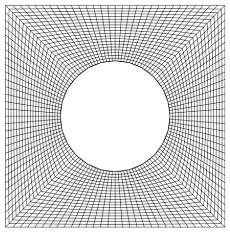
The physics-informed loss function is a valuable tool for using physical insights to inform the training of deep learning models, which plays the most important role in PINNs [10]. Generally, the performance of ANNs highly depends on the construction of their loss function. In PINNs, such physical constraints, including both governing equations and boundary condition equations, are imposed upon the loss function in the form of a partial differential that is directly described by automatic differentiation. The incorporation of physical constraints into the loss function helps to reduce the complexity of the model, leading to improved generalization and better performance. Additionally, the physical constraints can be used to ensure that the model conforms to certain physical laws, ensuring that the model is providing reliable and correct predictions. Owing to the popular graph-based utilization of neural network libraries (e.g., TensorFlow and PyTorch), the automatic differentiation technique is easy to carry out, thus enabling the embedding of physics constraints in the loss function [23].

The physics-informed loss function,$\mathcal{L}$, including data loss and physics loss, can be written as follows:

$$\mathcal{L}={\mathcal{L}}_d+{\mathcal{L}}_p$$

(6)

where

$${\mathcal{L}}_d={\parallel u_i^{*}-{\widehat{u}}_i\parallel }_2^2$$

(7)

$${\mathcal{L}}_p={\parallel {\sigma }_{ij,j}+f_i\parallel }_2^2+{\parallel u_i-{\overline{u}}_i\parallel }_2^2+{\parallel {\sigma }_{ij}{n}_j-{\overline{f}}_i\parallel }_2^2$$

(8)

The symbol ${\widehat{u}}_i$ refers to the predicted displacement, which is a function of the input variables and represents the solution to the physical problem being studied. The symbol $u_i^{*}$ represents the actual values of some data. The notations in ${\mathcal{L}}_p$ have the same meanings as described in Section 2.1. In the context of this paper’s two-dimensional problem, the indices $i$ and $j$ correspond to either 1 and 2 or $x$ and $y$, respectively, and each index represents a component of a tensor.

Forward problems can be solved using ${\mathcal{L}}_p$ without any labeled data within physics domains. As for inverse problems, such as those related to identifying the Young’s modulus of an unknown material, ${\mathcal{L}}_d$ is required in addition to ${\mathcal{L}}_p$.

3. Validation Tests

A two-dimensional linear elastic problem, represented by a square plate with a hole subjected to a uniaxial load, was selected to illustrate the applicability of the PINN framework to modeling non-uniform deformation. The length of the square plate is 1.0 m, and it has a circular opening located in the center with a radius of 0.25 m (shown in Figure 2). The Young’s modulus $E$ and Poisson’s ratio $v$ are 1 MPa and 0.3, respectively. In our experiment, uniaxial normal displacement ${\overline{u}}_y=0.5$. was applied to the top edge, as shown in Figure 2. An open-holed plate is a commonly used structure for studying the mechanical behavior of different material types, such as composite materials and gradient materials. It can be used to clearly illustrate stress concentration and describe mechanical behavior under complex stress and has thus been widely used to calculate tensile strength, stress intensity factor, etc.

3.1. Forward Problems

Forward problems in solid mechanics involve predicting the mechanical response of a material subjected to boundary conditions, loads, and initial conditions, given its material properties. These problems are often used to simulate the behavior of materials or structures under different boundary conditions in order to gain a better understanding of their response, such as stress, strain, deformation, and displacement. Generally, these problems are typically solved using numerical techniques such as FEM and FDM, solving the equations of motions of the problem. Such techniques allow for the accurate application of boundary conditions, material properties, and other physical constraints. Here, we try to solve this forward problem in solid mechanics using the PINN approach.

The governing equations and the boundary condition equations for the plate problem are shown in Figure 2, and they can be expounded as follows:

Governing equations:

$$\left\{\begin{array}{l}\frac{E}{1-v^2}\left(\frac{{\partial }^2{u}_x}{\partial x^2}+\frac{1+\mu }{2}\frac{{\partial }^2{u}_y}{\partial x\partial y}+\frac{1-\mu }{2}\frac{{\partial }^2{u}_x}{\partial y^2}\right)+f_x=0\\ \frac{E}{1-v^2}\left(\frac{{\partial }^2{u}_y}{\partial y^2}+\frac{1+\mu }{2}\frac{{\partial }^2{u}_x}{\partial x\partial y}+\frac{1-\mu }{2}\frac{{\partial }^2{u}_y}{\partial x^2}\right)+f_y=0\end{array}\right.$$

(9)

Boundary conditions equations:

$$\left\{\begin{array}{l}\frac{E}{1-v^2}\left[l\left(\frac{\partial u_x}{\partial x}+\mu \frac{\partial u_y}{\partial y}\right)+m\frac{1-\mu }{2}\left(\frac{\partial u_y}{\partial x}+\frac{\partial u_x}{\partial y}\right)\right]={\overline{f}}_x\\ \frac{E}{1-v^2}\left[m\left(\frac{\partial u_y}{\partial y}+\mu \frac{\partial u_x}{\partial x}\right)+l\frac{1-\mu }{2}\left(\frac{\partial u_y}{\partial x}+\frac{\partial u_x}{\partial y}\right)\right]={\overline{f}}_y\end{array}\right.$$

(10)

where

$$l=cos\left(\mathit{n},\mathit{x}\right)$$

(11)

$$m=cos\left(\mathit{n},\mathit{y}\right)$$

(12)

In total, 1500 sample points were randomly generated across the whole domain, including both the interior computational domain and boundary computational domain, with about 20% of the sample points uniformly distributed at the boundary. Additionally, a fully connected neural network (FCN) was applied to predict $u_x$ and $u_y$, with eight hidden layers and 64 neurons per hidden layer, and tanh was here employed as the activation function throughout this study. The FEM-calculated results, achieved using the commercial software ABAQUS with a total mesh of 2400 elements (CPS4R in ABAQUS notation, shown in Figure 3), were used here to express the exact solution.

The training loss versus epoch plot (Figure 4) illustrates the convergence behavior of the PINN model over 10,000 training iterations. The plot shows a steady decrease in the training loss over the course of the training process, indicating that the model effectively learned the underlying physics and reduced the discrepancy between the predicted and true values. The training loss decreased rapidly in the initial epochs and then gradually stabilized to a low value, suggesting that further training may not result in significant improvements. Overall, the plot demonstrates that the PINN model is capable of efficiently learning complex physical phenomena with a relatively small number of training epochs.

The displacement fields ($u_x$ and $u_y$) calculated via the PINN approach are presented in Figure 5 and show satisfactory agreement with the results derived from the FEM. In order to more intuitively illustrate the differences between the displacement fields obtained by the FEM and PINN, an absolute error map is presented in Figure 6. As shown here, the PINN approach successfully predicted the displacements, while a maximum absolute error of only −0.00401 was found. Furthermore, the PINN approach can clearly capture the strain concentrations of the ${\epsilon }_{xx}$,${\epsilon }_{yy}$ and ${\epsilon }_{xy}$ fields at the boundaries of the computational domains of the plate and specifically near the edge of the hole (shown in Figure 7). Though the strain components could only be indirectly obtained via the derivation of the displacement components, the strain fields maintained good agreement with the FEM results, while only a minor discrepancy was found near the edge of the inner hole.

In order to quantitatively evaluate the performance of the PINN approach used in the displacement calculation, the horizontal and vertical displacement distributions, shown in the regions marked by a red line, were compared with those derived from the FEM calculations (Figure 8) and found to agree with each other well. Additionally, the results derived from the PINN approach to linear elastic solid mechanics exhibited excellent properties of symmetry.

Compared to the FEM, PINNs do not offer significant advantages in terms of computational accuracy and efficiency in forward problems [23]. However, PINNs are more flexible, as they can solve physical problems without the need for a mesh, giving them a greater advantage when dealing with complex geometries or high mesh requirements. Furthermore, after training, PINNs can save their network parameters for direct prediction without the need for retraining.

3.2. Inverse Problems

Inverse problems in solid mechanics aim to determine the unknown parameters of a material by observing some measurements of the system [37,38]. These measurements may be displacement, strain, stress, etc. Inverse problems can be useful in determining the parameters of a material when direct measurement is not possible, such as in material characterization or system identification, which are especially important for the analysis and identification of materials and structures. The parameters to be determined include the Young’s modulus, Poisson’s ratio, and other physical properties. Generally, inverse problems are much more difficult than forward problems involving the determination of the response for a given set of parameters. The difficulty arises from the fact that the measured response does not contain enough information to uniquely determine all the parameters and these equations for solid mechanics problems are typically non-linear. To guarantee a unique solution, one approach is to apply additional constraints to the input parameters. For instance, in the paper by Chen et al. [39], they employed a deep neural network inverse solution to recover pre-crash impact data of car collisions while enforcing physical constraints on the solution space. Specifically, they included a regularization term that penalized non-physical solutions, such as those with negative values for physical parameters. Additionally, Xie et al. [40] proposed a feed-forward neural network-based variational Bayesian learning method for the forensic analysis of traffic accidents. Their approach combined Bayesian inference and neural networks to assess the uncertainty of predicted solutions and provide a probabilistic evaluation of the results. This could aid in detecting multiple solutions and guaranteeing the uniqueness of the most probable solution. In summary, to ensure the uniqueness of solutions in inverse analyses utilizing PINNs, it is crucial to incorporate physical constraints and regularization techniques into the network’s architecture and estimate the uncertainty of the predicted solutions. These techniques can prevent the network from predicting non-physical solutions and guarantee the uniqueness of the most probable solution.

The inverse problem that we considered here was to identify the Poisson’s ratio $v$ (exact value: 0.3), which was taken as the unknown parameter in this section. The PINN takes the spatial coordinate $\mathit{x}$ as the input and outputs the corresponding value of $\mathit{u}$. In order to identify the Poisson’s ratio $v$, we simultaneously optimized the weights and biases of the neural network along with the Poisson’s ratio by minimizing the differences between the predicted and measured $\mathit{u}$ using the loss function, while using 200 points (marked by circles in Figure 9) randomly sampled from the interior of the computational domain for $\mathit{u}$ as the known data. To enforce the physics-based constraints, we also incorporated the boundary conditions and governing equation into the loss function. The boundary conditions and governing equations (the same as those introduced in the previous section) were taken as a priori. Accordingly, the aim here was to estimate the Poisson’s ratio $v$ from the 200 known points of $\mathit{u}$ within the interior of the computational domain. In order to examine the applicability of using a PINN to solve inverse problems, Gaussian-distributed noise [41] with a zero mean was generated for all the sampled points. Three different scales of noise were applied to $\mathit{u}$, i.e., (1) ${ϵ}_1$ ∼$N\left(0, 0.001\right)$, (2) ${ϵ}_2$ ∼$N\left(0, 0.005\right)$, and (3) ${ϵ}_3$∼$N\left(0, 0.01\right)$.

The limited-memory Broyden–Fletcher–Goldfarb–Shanno (L-BFGS) optimizer with a learning rate of 0.1 was used to train the PINN, with the number of training steps set as 2000.

Table 1. Comparison of different noise scales for inversion.

Noise Scale	Identified $\mathit{v}$	Deviation	Number of Iterations
${ϵ}_1$	0.29802	0.00198	1221
${ϵ}_2$	0.30758	0.00758	2523
${ϵ}_3$	0.32636	0.02636	3851

illustrates the values of $v$ that were identified for different scales of noise, with the initial $v$ used for inversion set as 0.8.

It can be seen that deviation increased with increases in noise scale. In general, the values of the converged Poisson’s ratio $v$, as derived from the PINN approach at different noise scales, were almost identical to the exact solution, which indicates the good performance of the PINN when used for inversion. When the PINN was applied to the ${ϵ}_1$ noise scale, it required 1221 iterations to finish training for the 2D inversion problem, while applying the same approach to the ${ϵ}_2$ and ${ϵ}_2$ noise scales required about 2523 and 3851 iterations, respectively. This indicates that noise scale has a strong effect on inversion efficiency.

We now seek to further verify the applicability of the PINN to inverse problems. Accordingly, a more challenging task designed to reveal the unknown physics law at play in displacement observations is presented here; said law is assumed to follow an exponential form:

$$v=v\left(x\right)=\alpha e^x$$

(13)

where $x$ donates the horizontal coordinate ranging from 0 to 1 and $\alpha$ donates the coefficient, set at the constant of $1/3$ in this problem. Exact displacement observations were generated using the FEM (using the mesh scheme shown in Figure 3) via Equation (13), implemented on ABAQUS via user-defined materials (UMATs). The goal is to predict the evolution law of $v$ based on the exact displacement observations and the assumption that $v$ is simply a function of $x$, whereby the specific form of $v\left(x\right)$ is a priori unknown. This task was challenging compared to the previous one of simply identifying an unknown parameter during training.

In order to approximate the exact evolutionary law of $v\left(x\right)$, an array $v_n$ with n elements was established, with the Poisson’s ratio set in the horizontal direction uniformly divided into $n$ layers. A schematic diagram of $v_n$ is shown in Figure 10, i.e., $v_i$ represents the Poisson’s ratio of $i$th layer. The values of $n$, representing the number of unknown parameters requiring identification, are set as 5, 10, and 15 during the inversion process, respectively. The details and parameters of the training follow those used in the previous study (Table 1). Similarly, $n$ parameters were optimized together with the weights and biases in the neural network during the training process.

The converged $v_n$ after inversion is shown in Figure 10. The circle, square, and triangle marks represent the results derived from the PINN with the values of $n$ set as 5, 10, and 15, respectively. The black line represents the exact solution obtained from Equation (13).

Figure 11a depicts the loss versus epoch curve ($n=10$) for a PINN model used to approximate $v\left(x\right)$. The curve demonstrates the convergence of the model, indicating that the model learned to fit the training data and approximate $v\left(x\right)$ accurately. The gradual decrease in loss with increasing epochs suggests that the model was learning and adapting to the problem over time and eventually converged to a stable solution. In general, the converged $v_n$ derived from the PINN showed good agreement with the exact solution (shown in Figure 11b), illustrating the capacity of the PINN when used to determine unknown physics laws from a complex non-linear system. As observable in Figure 10, the PINN approach successfully predicted the evolutionary law of the Poisson’s ratio as given by Equation (13), while a maximum discrepancy of only 0.131 was found when $n=15$. It can be inferred that $n=10$ is the best choice when seeking to solve this problem using a PINN. This is because, when the number of unknown parameters is too small, the $v_n$ usually fails to directly reflect the true evolution law. However, when too many parameters are required to be identified at the same time, the calculation accuracy suffers, which may limit the success of identifying the true physics laws.

To further test the ability of PINNs to handle inverse problems, we present an example of using a PINN to invert a non-homogeneous modulus field along the y direction (shown in Figure 12). The model used here was the same as the one used to invert for an unknown Poisson ratio distribution discussed earlier. We assume that the elastic modulus follows the distribution:

$$E=E\left(y\right)=4{\left(y-0.5\right)}^2+1$$

(14)

As seen from Equation (14), the modulus followed a quadratic distribution in the y direction. To solve this problem, we adopted a method of solving for the Poisson’s ratio, which is not discussed here for brevity.

The converged $E_n$ after inversion is shown in Figure 12. The circle, square, and triangle marks represent the results derived from the PINN with the values of $n$ set as 5, 10, and 15, respectively. The black line represents the exact solution obtained from Equation (14). The convergence curve of the training for this model is similar to that of the Poisson example and is thus not presented here.

From Figure 13, it is apparent that the three inversion results showed good agreement with the true result and were all capable of reflecting the distribution pattern of the true modulus. On the whole, it can be observed that when $n=10$, the degree of agreement between the inversion results was higher, which is highly consistent with the conclusion obtained from the inversion of the Poisson ratio distribution mentioned earlier. This example serves as further evidence of the powerful ability of PINNs in dealing with inverse problems.

Table 2. Inversion times for different examples using the FEM and PINN methods.

Example ID	FEM	PINN
1	17 s	14 s
2	625 s	63 s
3	674 s	66 s

presents the computation time required by the PINN and FEM methods for the three examples mentioned earlier, namely, the inversion of a single Poisson’s ratio, the inversion of a Poisson ratio distribution with an unknown form ($n=10$), and the inversion of a modulus field with an unknown form ($n=10$). For simplicity, we will label these three examples as 1, 2, and 3, respectively. In this study, we utilized the finite element model updating method (FEMU) to perform parameter inversion for these examples, based on the approach described in [42,43]. Notably, the differences in accuracy between the FEMU and PINN for the inverse problem were insignificant; therefore, we focused on comparing their computational efficiency. The experiments were conducted on a computer equipped with an Intel i7 processor (8-core) and 16 GB of RAM, and computations were accelerated by a GeForce RTX 2070 GPU.

Our results demonstrate that the PINN method achieved a remarkable reduction in computational time compared to the FEM, especially in scenarios that required the inversion of multiple parameters. As shown in Table 2, the inversion time with the PINN was up to 90% lower than that with the FEM. For instance, the inversion time for Examples 2 and 3 was reduced from 625 s and 674 s with the FEM to 63 s and 66 s with the PINN, respectively. This highlights the innovative potential of the PINN method in solid mechanics and emphasizes its capability for efficient and accurate inverse analysis. By minimizing computational time, the PINN method provides researchers with the opportunity to expedite their investigations and make informed decisions promptly. These results are promising and demonstrate a significant advancement toward establishing PINNs as reliable and efficient tools for inverse analyses in solid mechanics.

4. Conclusions

The accurate modeling of the non-uniform deformation of materials is essential to the description and analysis of their complex mechanical behaviors, which can be exploited in digital twins, for example. In this study, a PINN-based method involving the tension testing of an open-holed square plate is proposed to solve solid mechanics problems via the displacement method, importing both forward problems and inverse problems. The following are the main conclusions of this study:

• A PINN framework comprising a simple FNN structure and a conventional physics-informed loss function can perform well in non-uniform deformation predictions and capture strain concentration well within the whole computational domain;
• The two case studies conducted to verify the effectiveness of this approach in identifying unknown physics laws show its promise and power in addressing inverse problems related to computational mechanics;
• Using the PINN method, the distribution of the unknown parameters of material can be identified via a single uniaxial test though one training session, thus avoiding the complexity of conventional uniaxial tests performed on several specimens.

References

1. Davydov, O.; Oanh, D.T.; Tuong, N.M. Improved stencil selection for meshless finite difference methods in 3D. J. Comput. Appl. Math. 2023, 425, 115031. [Google Scholar] [CrossRef]
2. Xiong, Z.; Wang, X.; He, M.; Benabou, L.; Feng, Z. Investigation on thermal conductivity of silver-based porous materials by finite difference method. Mater. Today Commun. 2022, 33, 104897. [Google Scholar] [CrossRef]
3. Sílvia, R.C.; Lauro, C.H.; Ana, H.; Davim, J.P. Development of FEM-based digital twins for machining difficult-to-cut materials: A roadmap for sustainability. J. Manuf. Process. 2022, 75, 739–766. [Google Scholar] [CrossRef]
4. Shetty, N.; Shahabaz, S.; Sharma, S.; Shetty, S.D. A review on finite element method for machining of composite materials. Compos. Struct. 2017, 176, 790–802. [Google Scholar] [CrossRef]
5. Badia, S.; Caicedo, M.A.; Martín, A.F.; Principe, J. A robust and scalable unfitted adaptive finite element framework for nonlinear solid mechanics. Comput. Methods Appl. Mech. Eng. 2021, 386, 114093. [Google Scholar] [CrossRef]
6. Nouzil, I.; Eltaggaz, A.; Deiab, I.; Pervaiz, S. Numerical CFD-FEM model for machining titanium Ti-6Al-4V with nano minimum quantity lubrication: A step towards digital twin. J. Mater. Process. Technol. 2023, 312, 117867. [Google Scholar] [CrossRef]
7. Wainberg, M.; Merico, D.; Delong, A.; Frey, B.J. Deep learning in biomedicine. Nat. Biotechnol. 2018, 36, 829–838. [Google Scholar] [CrossRef]
8. Ching, T.; Himmelstein, D.S.; Beaulieu-Jones, B.K.; Kalinin, A.A.; Do, B.T.; Way, G.P.; Ferrero, E.; Agapow, P.-M.; Zietz, M.; Hoffman, M.M.; et al. Opportunities and obstacles for deep learning in biology and medicine. J. R. Soc. Interface 2018, 15, 20170387. [Google Scholar] [CrossRef] [Green Version]
9. Rackauckas, C.; Ma, Y.; Martensen, J.; Warner, C.; Zubov, K.; Supekar, R.; Skinner, D.; Ramadhan, A.; Edelman, A. Universal Differential Equations for Scientific Machine Learning. arXiv 2020, arXiv:2001.04385. [Google Scholar]
10. Raissi, M.; Perdikaris, P.; Karniadakis, G. Physics-informed neural networks: A deep learning framework for solving forward and inverse problems involving nonlinear partial differential equations. J. Comput. Phys. 2019, 378, 686–707. [Google Scholar] [CrossRef]
11. Sun, L.; Gao, H.; Pan, S.; Wang, J.-X. Surrogate modeling for fluid flows based on physics-constrained deep learning without simulation data. Comput. Methods Appl. Mech. Eng. 2020, 361, 112732. [Google Scholar] [CrossRef] [Green Version]
12. Jin, X.; Cai, S.; Li, H.; Karniadakis, G.E. NSFnets (Navier-Stokes flow nets): Physics-informed neural networks for the incompressible Navier-Stokes equations. J. Comput. Phys. 2020, 426, 109951. [Google Scholar] [CrossRef]
13. He, Z.; Ni, F.; Wang, W.; Zhang, J. A physics-informed deep learning method for solving direct and inverse heat conduction problems of materials. Mater. Today Commun. 2021, 28, 102719. [Google Scholar]
14. Zobeiry, N.; Humfeld, K.D. A physics-informed machine learning approach for solving heat transfer equation in advanced manufacturing and engineering applications. Eng. Appl. Artif. Intell. 2021, 101, 104232. [Google Scholar] [CrossRef]
15. Smith, J.D.; Azizzadenesheli, K.; Ross, Z.E. EikoNet: Solving the Eikonal Equation with Deep Neural Networks. IEEE Trans. Geosci. Remote Sens. 2020, 59, 10685–10696. [Google Scholar] [CrossRef]
16. Rasht-Behesht, M.; Huber, C.; Shukla, K.; Karniadakis, G.E. Physics–Informed Neural Networks (PINNs) for Wave Propagation and Full Waveform Inversions. J. Geophys. Res. Solid Earth 2022, 127, e2021JB023120. [Google Scholar] [CrossRef]
17. Song, C.; Alkhalifah, T.A. Wavefield Reconstruction Inversion via Physics-Informed Neural Networks. IEEE Trans. Geosci. Remote Sens. 2021, 60, 1–12. [Google Scholar] [CrossRef]
18. Shukla, K.; Di Leoni, P.C.; Blackshire, J.; Sparkman, D.; Karniadakis, G.E. Physics-Informed Neural Network for Ultrasound Nondestructive Quantification of Surface Breaking Cracks. J. Nondestruct. Eval. 2020, 39, 1–20. [Google Scholar] [CrossRef]
19. Rao, C.; Sun, H.; Liu, Y. Physics-Informed Deep Learning for Computational Elastodynamics without Labeled Data. J. Eng. Mech. 2021, 147, 04021043. [Google Scholar] [CrossRef]
20. Haghighat, E.; Raissi, M.; Moure, A.; Gomez, H.; Juanes, R. A physics-informed deep learning framework for inversion and surrogate modeling in solid mechanics. Comput. Methods Appl. Mech. Eng. 2021, 379, 113741. [Google Scholar] [CrossRef]
21. Niu, S.; Zhang, E.; Bazilevs, Y.; Srivastava, V. Modeling finite-strain plasticity using physics-informed neural network and assessment of the network performance. J. Mech. Phys. Solids 2023, 172, 105177. [Google Scholar] [CrossRef]
22. Kissas, G.; Yang, Y.; Hwuang, E.; Witschey, W.R.; Detre, J.A.; Perdikaris, P. Machine learning in cardiovascular flows modeling: Predicting arterial blood pressure from non-invasive 4D flow MRI data using physics-informed neural networks. Comput. Methods Appl. Mech. Eng. 2020, 358, 112623. [Google Scholar] [CrossRef]
23. Zeng, S.; Cai, Y.; Zou, Q. Deep neural networks based temporal-difference methods for high-dimensional parabolic partial differential equations. J. Comput. Phys. 2022, 12, 111503. [Google Scholar] [CrossRef]
24. Sirignano, J.; Spiliopoulos, K. DGM: A deep learning algorithm for solving partial differential equations. J. Comput. Phys. 2018, 375, 1339–1364. [Google Scholar] [CrossRef] [Green Version]
25. Ling, J.; Jones, R.; Templeton, J. Machine learning strategies for systems with invariance properties. J. Comput. Phys. 2016, 318, 22–35. [Google Scholar] [CrossRef] [Green Version]
26. Wang, R.; Kashinath, K.; Mustafa, M.; Albert, A.; Yu, R. Towards Physics-informed Deep Learning for Turbulent Flow Prediction. Comput. Phys. 2020, 10, 1457–1466. [Google Scholar]
27. Blakseth, S.S.; Rasheed, A.; Kvamsdal, T.; San, O. Combining physics-based and data-driven techniques for reliable hybrid analysis and modeling using the corrective source term approach. Comput. Methods Appl. Mech. Eng. 2021, 379, 113759. [Google Scholar] [CrossRef]
28. Zhu, Y.; Zabaras, N.; Koutsourelakis, P.S.; Perdikaris, P. Physics-constrained deep learning for high-dimensional surrogate modeling and uncertainty quantification without labeled data. J. Comput. Phys. 2019, 394, 56–81. [Google Scholar] [CrossRef] [Green Version]
29. Yin, M.; Zhang, E.; Yu, Y.; Karniadakis, G.E. Interfacing finite elements with deep neural operators for fast multiscale modeling of mechanics problems. Comput. Methods Appl. Mech. Eng. 2022, 402, 115027. [Google Scholar] [CrossRef]
30. Giuseppe, C.; Matthias, T. Solving the quantum many-body problem with artificial neural networks. Science 2017, 355, 602. [Google Scholar]
31. Brodnik, N.R.; Muir, C.; Tulshibagwale, N.; Rossin, J.; Echlin, M.P.; Hamel, C.M.; Kramer, S.L.B.; Pollock, T.M.; Kiser, J.D.; Smith, C.; et al. Perspective: Machine learning in experimental solid mechanics. J. Mech. Phys. Solids 2023, 173, 105231. [Google Scholar] [CrossRef]
32. Li, Z.; Kovachki, N.; Azizzadenesheli, K.; Liu, B.; Bhattacharya, K.; Stuart, A.; Anandkumar, A. Fourier Neural Operator for Parametric Partial Differential Equations. arXiv 2020, arXiv:2010.08895. [Google Scholar]
33. Black, N.; Najafi, A.R. Learning finite element convergence with the multi-fidelity graph neural network. Comput. Methods Appl. Mech. Eng. 2022, 397, 115120. [Google Scholar] [CrossRef]
34. Timoshenko, S.P.; Gere, J.M. Theory of Elastic Stability; McGraw-Hill Education: New York, NY, USA, 1961. [Google Scholar]
35. Qu, D.; Tang, D. On control structure scheme of feedback linearization for nonlinear system based on ANN models and simulation researches. In Proceedings of the 2010 3rd International Congress on Image and Signal Processing, Yantai, China, 16–18 October 2010; pp. 3645–3649. [Google Scholar] [CrossRef]
36. Katageri, A.C.; Sheeparamatti, B.G. An ANN model of polymer based MEMS structures: A modal analysis approach. In Proceedings of the 2014 International Conference on Smart Structures and Systems (ICSSS), Chennai, India, 9 October 2014; pp. 112–117. [Google Scholar] [CrossRef]
37. Hamel, C.M.; Long, K.N.; Kramer, S.L.B. Calibrating constitutive models with full-field data via physics informed neural networks. Strain 2022, 59, e12431. [Google Scholar] [CrossRef]
38. Sun, X.; Yue, L.; Yu, L.; Shao, H.; Peng, X.; Zhou, K.; Demoly, F.; Zhao, R.; Qi, H.J. Machine Learning-Evolutionary Algorithm Enabled Design for 4D-Printed Active Composite Structures. Adv. Funct. 2021, 32, 2109805. [Google Scholar] [CrossRef]
39. Chen, Q.; Xie, Y.; Ao, Y.; Li, T.; Chen, G.; Ren, S.; Wang, C.; Li, S. A deep neural network inverse solution to recover pre-crash impact data of car collisions. Transp. Res. Part C Emerg. Technol. 2021, 126, 103009. [Google Scholar] [CrossRef]
40. Xie, Y.; Wu, C.T.; Li, B.; Hu, X.; Li, S. A feed-forwarded neural network-based variational Bayesian learning approach for forensic analysis of traffic accident. Comput. Methods Appl. Mech. Eng. 2022, 397, 115148. [Google Scholar] [CrossRef]
41. Ye, Y.; Li, Y.; Ouyang, R.; Zhang, Z.; Tang, Y.; Bai, S. Improving machine learning based phase and hardness prediction of high-entropy alloys by using Gaussian noise augmented data. Comp. Mater. Sci. 2023, 223, 112140. [Google Scholar] [CrossRef]
42. Liu, G.; Wang, L.; Yi, Y.; Sun, L.; Shi, L.; Ma, S. Inverse identification of graphite damage properties under complex stress states. Mater. Des. 2019, 183, 108135. [Google Scholar] [CrossRef]
43. Liu, G.; Wang, L.; Yi, Y.; Sun, L.; Shi, L.; Jiang, H.; Ma, S. Inverse identification of tensile and compressive damage properties of graphite material based on a single four-point bending test. J. Nucl. Mater. 2018, 509, 445–453. [Google Scholar] [CrossRef]
Figure 1. A physics-informed neural network containing two main components: an artificial neural network and a physics-informed loss function.
Applsci 13 04539 g001
Figure 2. Diagram of an open-holed square plate under a uniaxial load.
Applsci 13 04539 g002
Figure 3. Mesh scheming in FEM.
Applsci 13 04539 g003
Figure 4. Training loss versus epoch.
Applsci 13 04539 g004
Figure 5. Comparison of the calculated displacement fields (left: FEM; right: PINN) of the in-plain stretching-related solid mechanics problem.
Applsci 13 04539 g005
Figure 6. Absolute error derived from the PINN framework for displacements.
Applsci 13 04539 g006
Figure 7. Comparison of the obtained strain fields (left: FEM; right: PINN) of the in-plain stretching-related solid mechanics problem.
Applsci 13 04539 g007
Figure 8. Comparison of the obtained displacement, represented by the red line (from left/bottom to right/top). (a) horizonal and (b) vertical displacement distributions of the marked regions.
Applsci 13 04539 g008
Figure 9. Training samples for u .
Applsci 13 04539 g009
Figure 10. Schematic diagram for v n uniformly distributed in the x direction.
Applsci 13 04539 g010
Figure 11. (a) Training loss versus epoch ( n = 10 ); (b) Converged v n ( n = 5 ,   10 , and 15 ) obtained from the PINN in the x direction.
Applsci 13 04539 g011
Figure 12. Schematic diagram for E n uniformly distributed in the y direction.
Applsci 13 04539 g012
Figure 13. Converged E n ( n = 5 ,   10 , and 15 ) obtained from the PINN in the y direction.
Applsci 13 04539 g013