Featured Application
Implementation of an integrated EWMS using a model predictive control strategy based on fuzzy optimization. The proposed EWMS is used to optimize irrigation for an indoor greenhouse crop.
Abstract
Rural communities usually settle in territories where crop self-consumption is the main source of sustenance. In this context, climate change has made these environments of crop control susceptible to water shortages, impacting crop yields. The implementation of greenhouses has been proposed to address these problems, together with strategies to optimize water and energy consumption. In this study, an energy–water management system based on a model predictive control strategy is proposed. This control strategy consists of a fuzzy optimizer used to determine the optimal consumption from isolated microgrids considering the local resources available. The proposed controller is implemented on two timescales. First, medium-term optimization over one month is used to estimate the necessary water demand required to support crop growth and a high yield. Second, short-term optimization is used to determine the optimal climate conditions inside the greenhouse for managing crop irrigation, refilling the reserve water tank, and providing ventilation. Experiments were conducted to test this approach using a case study of an isolated community. For such a case, energy consumption was reduced, and the irrigation process was optimized. The results indicated that the proposed controller is a viable alternative for implementing intelligent management systems for greenhouses.
1. Introduction
In managing the energy–water nexus, modeling the relationships between energy and water in uncertain scenarios is essential when considering applications in small settlements that lack proper access to these resources. This is important because the uncertainties can significantly impact the optimal course of action to maintain the sustainability of the nexus. For example, climate change can generate weather conditions that produce water shortages [1], impacting overall crop yields. Additionally, these adverse climate conditions could increase aquifer water extraction to comply with the demand, thus influencing the future availability of water resources. Therefore, in these scenarios, a sustainable management system should incorporate techniques that support efficient water use, such as the use of recycling or treatment plants. Additionally, the total energy cost should be minimized. Therefore, the design of an energy–water management system for efficiently managing the available resources of small settlements should include all characteristics of the community, especially when greenhouses are established [2].
In this work, an energy–water management system (EWMS) based on model predictive control (MPC) is proposed for the José Painecura Hueñalihuen Mapuche indigenous community. This isolated community is located in southern Chile and is affected by connection failures. Additionally, the connection costs with the central Chilean electricity distribution network are high.
When evaluating the performance of an energy–water nexus, it is crucial to maximize efficiency and sustainability [3] while also meeting the demands of each system component. The physical characteristics of the system, such as the maximum volume of water storage, photovoltaic power capacity, and crop surface area, can be manipulated to solve this problem [4]. In [5], a three-layer hierarchical predictive control approach was used for wastewater management. In this approach, an upper layer performed long-term management by sending setpoints to lower layers for short-term actions. In [1], an autonomous greenhouse irrigation system based on photovoltaic power was designed, and the crop yield results were better than those in an unmanaged case. In [6], a photovoltaic irrigation system with no storage tank was considered, and the management system made decisions based on predefined demand requirements. Although the results showed that the system met the irrigation demands, the authors did not evaluate the crop yield or the system’s performance in adverse climate conditions. Some solutions have also been based on nonlinear approaches due to the complexity of these systems. For example, in [7], a photovoltaic irrigation system without a water storage tank was proposed. The irrigation deficit for various crops was handled using a genetic algorithm that minimized the cost of a photovoltaic plant. Another example was provided by [8], who used a fuzzy control strategy to optimize PV irrigation for tomato crops according to the estimated water demand.
Some works have also studied the possibility of integrating energy–water management systems into the overall grid. For example, in the PV system proposed in [9], with the constraint of minimizing the irrigation deficit, excess energy could be bought or sold to the overall grid, and a model was trained to minimize energy costs. Finally, in [10], a robust control approach was used to optimize the performance of a PV irrigation system connected to an overall grid, where the energy cost and irrigation deficit were minimized considering a worst-case scenario for the future price of energy from the grid.
Other factors that people should consider in EWMS design include the economic optimization of the system dimensions. Here, the challenge lies in minimizing implementation and operation costs while complying with the water and energy demands of crops in different climate scenarios. The authors of [11] proposed a genetic algorithm solution to optimize the sizing of PV irrigation systems while minimizing implementation costs and irrigation deficits. The results displayed better convergence than those of traditional optimizers, but the optimized system was characterized by low-efficiency energy usage. The authors of [12] designed a PV irrigation system that was optimized with a genetic algorithm and considered the irrigation demand, total system cost (implementation and operation), and income obtained from selling crops based on the total crop yield. The results showed that the proposed method reduced the overall system size, thereby increasing the economic feasibility. The authors of [13] proposed a technological-economic optimization model to minimize the life cycle cost of a PV irrigation system while minimizing the probability of energy deficiency. Additionally, the authors of [14] applied a centralized MPC to optimize water and energy considering the relevant water requirements and energy costs. Finally, the authors of [15] proposed a decision support system that maximized profit by determining the optimal combination of desalinated and brackish water for irrigation.
Taking into account these previous works, the main contributions of the present work are as follows:
- Neural networks and phenomenological models are used to predict the climatic variables that usually affect crop yields.
- A new controller design that integrates elements from energy and water management systems is proposed. This integrated control strategy is established to control crops in greenhouses in the short and medium terms.
- A climate regulator is implemented based on the openness of windows. Notably, the proposed controller design is based on concepts from model predictive control, and the optimal control actions are performed. Additionally, the proposed design includes fuzzy optimization for handling multiple control objectives and constraints by considering the uncertainty of the predicted climatic variables.
The novelties of this work are as follows:
- The integrated EWMS is applied for the operation of a semiclosed greenhouse. Previous works only applied EWMSs to open-field crops.
- Fuzzy optimization is included in the designed model predictive control scheme in the EWMS. As mentioned above, with fuzzy optimization, the model predictive control strategy can handle multiple control objectives and constraints, even when the system is affected by uncertainties.
This paper is structured as follows. Section 2 presents the details of the base methods considered as the background for the implementation of autoregressive models for the disturbance signals and the design of the model predictive controller. Section 3 describes the problem statement for applying the EWMS to greenhouse crops. Section 4 details how the predictions of the different climate variables that affect the greenhouse are handled. Section 5 presents the formulation of the MPC for implementing the EWMS over the short and medium terms. Section 6 describes the case study considered in this research, and Section 7 provides the corresponding simulation results. Finally, this work ends with Section 8, where the main conclusions based on the simulation results are discussed.
2. Background
The control strategy designed for implementing the EWMS relied on previous concepts from three frameworks: neural network modeling, model predictive control, and fuzzy optimization. The main concepts for each framework are presented below.
2.1. Neural Networks
A neural network predictive model is based on an autoregressive prediction strategy that uses artificial intelligence for modeling signals and systems. This model was selected because of its known characteristics as a universal approximator and its acceptable accuracy when predicting climate signals with stochastic behavior, as reported in the literature [16]. There are several possible structures for implementing a network; however, a multilayer perceptron (MLP) was considered in this work. This structure consists of two layers (a hidden layer and an output layer). The final output of this network is given by the following equation:
where is the net output for input ; and are the numbers of neurons in the hidden and input layers, respectively; and are the weights of the connections between input neuron i and hidden neuron j and hidden neuron j and the output neuron, respectively; and b are biases related to hidden neuron j and the output neuron, respectively; and, finally, f is the activation function.
2.2. Model Predictive Control
The EWMS design presented in this work is based on model predictive control (MPC). Notably, MPC has been used in the literature to improve the operation of systems based on optimizing future system behavior in regard to future control actions [17]. For this controller design, a discrete-time model of the system is required to predict future behavior. The future control actions are then determined by optimizing an objective function with constraints for the manipulated and controlled variables. Then, only the first action of the optimal future control is applied during the current time step. In the next time step, a new optimal sequence is obtained (rolling horizon). In general, the MPC optimization problem solved at each instant is given by:
where is the j-step-ahead prediction for the controlled variable, which is given by nonlinear prediction model f. Additionally, is the cost associated with the predicted output, is the reference value for the controlled variable, is the cost associated with the control action, and is the weighting factor. Finally, and are the prediction and control horizons, respectively.
2.3. Fuzzy Optimization
Fuzzy optimization is an optimization strategy that uses fuzzy logic to evaluate the performance of the objective function. This methodology was selected because it allows the MPC to fully consider the control objectives and constraints. Additionally, with fuzzy optimization, the MPC can consider the uncertainty associated with predicting the climatic variables. An example of its use was provided by [18]. When applied to MPC functions, and take the form of the complements to the membership functions. The MPC objective can be expressed as follows:
where and are complements for membership functions related to the tracking error and the control action, respectively.
3. Problem Statement
Achieving proper water and energy rationing is a relevant problem that must be overcome during the implementation of crop control systems in greenhouses. Additionally, the effects of climate change and trends in water scarcity must be considered, as they vary between different regions of the world. Therefore, to improve the operation of greenhouse systems, a control strategy that supports the optimal management of water and energy resources is proposed. Specifically, an integrated EWMS was designed based on MPC, and energy and water use were assessed from two temporal perspectives: a short-term perspective in which energy consumption is optimized for the next two days, and a medium-term perspective in which the water is managed for the next 28 days.
As shown in Figure 1, the water available for daily irrigation comes from a water tank installed in the greenhouse. Thus, for the medium-term objective associated with the WMS, the system controls the reference value for daily irrigation , which must be set by the controller based on the expected volume of water stored in the tank , the amount of water lost via evapotranspiration, and the previous amount of irrigated water used.
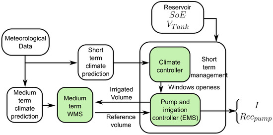
Figure 1.
EWMS diagram.
Moreover, in the short term, the controller needs to optimize energy use to maintain proper climate conditions (such as temperature and humidity ) to grow crops. In the greenhouse system used in this work, the controller requires electrical energy to operate the different actuators available, such as for the water pump used to refill the tank (binary variable—0 for closed and 1 for open); perform valve regulation to control the amount of water used for irrigation I (continuous variable—0 for no irrigation and 1 for irrigation for a full sample time); and control the openness of windows (binary variable—0 for closed and 1 for open). Here, all the energy necessary to operate this system comes from a photovoltaic system with a battery backup subsystem installed in the greenhouse. Thus, the short-term goal of the controller is to comply with the water use requirements at the medium-term scale while maintaining appropriate climate conditions and safe values of the state of energy to ensure an optimized battery lifespan.
Due to the stochastic behavior of the external climate conditions, the optimal management of future water use requires the proper characterization of the air temperature , solar irradiance , and external humidity . In this work, neural networks were used to provide information to the controller about future scenarios and climate conditions. Wind speed was also needed to implement this controller; however, due to the high uncertainty associated with the future values of this signal and the limited amount of data available for running models, a moving average for predictions in the short term was adopted. Then, the optimal management of water and energy use was realized by running two model predictive controls: one for the short-term objectives and another for the medium-term water management objectives. For both MPC blocks, the internal variables of the greenhouse were considered by using approximations of the relevant phenomenological models available in the literature, and the ground temperature was required in these models.
As shown in Figure 1, the prediction of the climate conditions at both the medium and short terms plays an essential role in supporting the management of available resources for the greenhouse. In the next section, the strategies used to predict the internal and external climate conditions are explained in detail.
Below, we summarize the controllers presented in Figure 1. Short-term climate prediction uses meteorological data from outside (, , , and ) and inside (, , and ) the greenhouse, as well as the window openness (), to generate meteorological data for the next two days every ten minutes. On the other hand, medium-term climate prediction uses this information to generate daily meteorological data for the next 28 days each day. Short-term climate prediction is used by the climate controller for short-term management to set future values of window openness for the next two days, while medium-term prediction is used by the medium-term WMS to determine daily irrigation volumes () for the next 28 days. Given the irrigation objective and estimates of future window openness based on meteorological data, the pump and irrigation controller (EMS) decides when and how much to irrigate (I) and when to activate the pump () for the next 48 h while considering the availability of water and energy . At the end of a day, the short-term management systems report back to the medium-term WMS the amount of water that was used for irrigation during the day.
4. Climate Predictions
As mentioned in Section 3, the control design proposed in this work considers short- and medium-term predictions. First, the short-term forecast of the weather conditions for the next 48 h is used to operate the EMS, with a sample time of 10 min. Then, the medium-term prediction spans the next 28 days, with a sample time of 1 day. These medium-term predictions are used to manage the WMS, which provides the water levels that are used later by the short-term manager for irrigation.
4.1. Short-Term Climate Prediction
From the short-term perspective, predicting future climate conditions is a crucial part of the EMS, because the internal weather in the greenhouse affects both the irrigation constraints and the control objective. Therefore, these variables can be classified into two categories: external and internal. The external variables associated with the weather outside the greenhouse are solar radiation, wind speed, external temperature, and external relative humidity. Additionally, the internal variables correspond to the greenhouse temperature, relative humidity, and subterranean temperature. In this work, different strategies were used to predict the internal and external variables, and they are explained below.
4.1.1. Prediction of External Climatic Variables
Neural network models were considered for predicting the future climate conditions outside the greenhouse. The training procedure for these models was implemented with meteorological data, such as historical measurements of ambient temperature , relative humidity , and solar irradiance . Then, for each of those climatic signals, a different neural network was trained so that the controller had an independent model available for each variable.
The networks were designed to use up to 144 regressors (equivalent to 1 day of information). Each network was designed with a total of two layers: one hidden and one output layer. In the case of the hidden layer, a minimum of 40 neurons and a maximum of 200 neurons were considered.
Based on the future values predicted for the external climate conditions with the neural networks, the proposed method could be applied to estimate the internal climatic variables for the greenhouse with the strategy explained in the next subsection.
4.1.2. Prediction of Internal Climatic Variables
Phenomenological equations and the predictions of the external variables provided by the neural networks were used to predict the internal climatic variables that affect short-term greenhouse behavior. This was carried out because the greenhouse did not contain instrumentation that could provide real climate data inside the greenhouse, so a phenomenological model was used to represent their behavior. The model was based on the gain and loss in heat and water vapor, similar to the models used in [19,20,21]. The model considered in this work was based on that used in [22,23], where the relationship between the temperature in the greenhouse , the underground temperature , and the absolute humidity was established considering heat and water vapor exchange. However, this equation could not be applied directly in the control system, because the controller proposed in this work required predictions with a large sampling time . The precision of the predictions would be low if the phenomenological model was applied with the same sampling step as the controller. Therefore, to avoid a loss in accuracy, the phenomenological model was used with the sampling time , such that . Therefore, the dynamics of each internal climatic condition were encompassed by the auxiliary variables , , and , which were used to obtain the values , , and required by the controller. The auxiliary variables represent estimated values of the greenhouse temperature, ground temperature, and greenhouse absolute humidity based on samples. Thus, the phenomenological model used in this work for the internal temperatures is defined as:
where is the index of the intermediate steps used to calculate the auxiliary variables available within a given sampling time. In Equation (6), the value is the heat exchanged, which is computed as:
where is the heat gained via radiation in W, defined as the sum of the solar radiation that enters the greenhouse and the thermic radiation from the greenhouse’s structure . is the heat exchange via conduction and convection, which is defined as:
with being the area of the external surface of the greenhouse structure, the convective heat transfer coefficient, the temperature inside the greenhouse, and the temperature measured outside.
Additionally, in Equation (8), is the heat exchange related to air renovation, which is represented by the following relationship between the temperature () and humidity () measured inside and outside the greenhouse:
where are constants determined by the air renovation rate and the characteristics of the greenhouse, following the equations described in [22]. is the heat exchange with the ground, which is described by:
where is the ground thermal conductivity, is the area of the ground surface in the greenhouse in m, and is the depth of temperature measurements in the soil. Finally, is the heat loss from evapotranspiration, represented by:
with being the latent heat of water, the potential evapotranspiration of crop c, and the corresponding crop’s area.
Additionally, in Equations (6) and (7), the constants and are the air and soil densities in kg/m, respectively; , , and denote the specific heat of dry air, water vapor, and the soil in J kgK, respectively; and, finally, is the air mass volume in the greenhouse.
The phenomenological model used for internal humidity estimation is defined as:
where is the total humidity variation. Additionally, in (14), corresponds to the absolute humidity variation via air exchange, which is computed as:
where is the air renovation rate. represents the absolute humidity variation via evapotranspiration, which is obtained using:
similar to the expression in Equation (12) for the heat loss case. Finally, is the absolute humidity variation via condensation, which is obtained based on:
where is a constant that was computed in [24] based on the area of the greenhouse, and is the temperature of the greenhouse cover.
At this point, the different models presented above could be used to obtain the climate predictions necessary for the short-term control of the greenhouse. However, some elements of the control strategy required medium-term predictions to obtain adequate references for water use in the greenhouse. In this case, it is not recommended to use the same kind of model because of the loss in precision when trying to obtain predictions far into the future. The process of medium-term prediction is described in the following subsection.
4.2. Medium-Term Climate Prediction
The main objective of medium-term climate prediction is to estimate the reference evapotranspiration daily for the next 28 days; this is required because these estimates play an important role in the WMS, as described in detail in the next section. Here, it was possible to reduce the needed information to the following variables: net radiation in the greenhouse , wind speed at height z , maximum greenhouse temperature , minimum greenhouse temperature , maximum greenhouse relative humidity , and minimum greenhouse relative humidity . For the first two days, it was possible to reuse the short-term prediction results; however, for subsequent days, other strategies are used.
To estimate , the following equations are used:
where and are the absorptivity and transmissivity coefficients for the greenhouse structure, respectively; is the absorptivity coefficient of the crops and soil and is proportional to the amount of ground cover; and is the average radiation inside the greenhouse on day k. The second term of (19) is a transformation factor that allows Wm to be transformed to MJ mday; this factor considers the number of seconds in a day and the conversion factor from units to Mega units. Additionally, and correspond to the area of the greenhouse floor and cover, respectively. In (20), the solar irradiance is the mean irradiance predicted for day k using a moving average.
A fixed value is used for future wind speed and, consequently, . This value is calculated as follows:
where is the average openness of windows during simulations, and is the average wind speed at a height of 2 m.
Finally, the estimated averages for the first two days predicted with the short-term models are used for the greenhouse temperature and the relative humidity. Thus, the values , , , and are fixed for all and equal to the average of values on the first and second days of the prediction horizon (e.g., for , is the average value between and ). This approach was used because the predictions provided by the model are less accurate in the medium term than in the short term due to the high stochasticity of the climatic variables and the limited availability of data for establishing long-term predictive models.
It was assumed that all of these variables could be regulated with greenhouse climate control. Therefore, their behavior should be the same across the prediction horizon under similar conditions.
With the predictive models for the short and medium terms, the greenhouse control could be established. In the following section, the details of climate control and the energy and water management systems are provided.
5. Model Predictive Control Strategies for the EWMS
The proposed greenhouse control system comprises three systems at two scales (short and medium). These three systems are the climate controller, a pump and irrigation controller (EMS), and a medium-term WMS. All of these systems are operated based on the solutions to optimization problems and the concepts of model predictive control. Below, the elements considered for implementing each predictive model controller are presented.
5.1. Short Term
Short-term management is separated into two controllers: the climate controller and the pump and irrigation controller (EMS). Every ten minutes, the climate controller minimizes its objective function (22) based on meteorological data, external climate predictions, and the phenomenological model of the greenhouse. Then, the climate controller sends a projection of the irradiance and greenhouse temperature to the EMS according to the optimal decision achieved for the openness of the windows. Based on this projection, as well as the values of resources available (the state of the battery charge and the volume of water available in the greenhouse tank) and the daily irrigation objective from medium-term management, the EMS controller minimizes the objective function (23). For both controllers, the objective functions (22) and (23) were solved in this work using particle swarm optimization (PSO). A summary of this interaction between the two short-term controllers is presented in Figure 2.
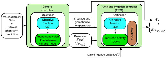
Figure 2.
Short-term management optimization flow chart, where PSO is used for both optimizations.
5.1.1. Climate Controller
With the predictive climate models presented in Section 4, it was possible to design a model predictive control strategy for greenhouse climate conditions. This strategy included a predictive controller with a 48 h horizon to determine the openness of windows in the future. This design had the advantages of being low-cost and able to appropriately regulate greenhouse climate conditions.
For the successful regulation of greenhouse conditions, future decisions regarding the openness of windows () were obtained by minimizing the following fuzzy objective function:
which was defined based on several fuzzy membership functions and the concept of fuzzy optimization [18,25]. In Equation (22), the objective function includes three main fuzzy membership functions , which are used to evaluate each of the control objectives defined. In particular, is the optimal range for the greenhouse temperature around a given reference value . The function represents the acceptable range for the differences between the greenhouse humidity and the reference value . The third membership function represents the penalization term for the number of changes in the window state. These three membership functions are used to simultaneously maintain temperature and humidity at desired values while opening or closing as few windows as possible.
The trapezoidal shapes of the membership functions for temperature and humidity can be observed in Figure 3; they were based on the definitions of temperature and humidity limits for tomatoes presented in [22,26]. These limits were defined for a security zone and a normal operation zone, and their values are reported in Table 1. To determine which membership function to use for temperature, the controller considers any instance with 100 Wm each day at an hourly scale, and 100 Wm is used as the reference condition at night. Moreover, the membership function for window openness is plotted as a simple sloped line, because linear penalization is sufficient in this case.
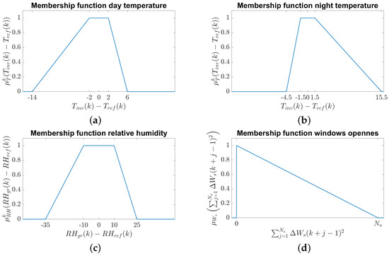
Figure 3.
Membership functions. (a) Daytime temperature; (b) night-time temperature; (c) relative humidity; (d) total window change.

Table 1.
Greenhouse climate limits.
5.1.2. Pump and Irrigation Controller (EMS)
Once the ideal climate conditions are achieved inside the greenhouse, it is necessary to manage the use of water and energy resources in the system. For this objective, the controller minimizes
to determine when the crop needs irrigation and how long that action has to be applied within the sample period (10 min). This decision regarding the volume of irrigation is represented by the variable . Additionally, from the minimization of (23), the model can determine when to use the pump to refill the water tank .
Three main components related to the conditions in the systems are included in the objective function (23). The first term is associated with the daily irrigation objective and is used to penalize the difference between the daily irrigation objective and the water used each day for irrigation. This difference is denoted as and varies each day. The values of for each possible day within a prediction horizon of 48 h are obtained with the following equations:
where is the volume of irrigation per second, and is the first of the prediction steps j for which an instant k coincides with a day change. Since H represents the number of prediction steps observed within 24 h, the predictions and are always associated with the first instant of a day. Additionally, Equations (24)–(26) show that the interactions among the objective functions vary each day because of the daily fluctuations in the irrigation objective . For example, in (24), on the first day, only the next prediction steps and the volume of water used on that day up to instant k are considered. Moreover, the third day in (26) is either not or partially considered, indicating that decision processes do not require information from the full third day. To compensate for this issue, the adjustment factor was added to decrease the weight of this decision. Additionally, in the first term of the objective function (23), the penalty parameters are defined as follows:
where and are the costs of excess and insufficient irrigation, respectively.
The second term in (23) is used to minimize the number of irrigation instances to avoid the excessive activation/deactivation of the actuators. In addition, the third term is used to minimize the power that the system uses to maintain operation. This third objective was included to ensure the proper functioning of the greenhouse system with optimal energy use.
At this point in the model predictive control design, monitoring the resource conditions, such as the volume of water in the water tank and the state of the battery charge, was important for achieving optimal system operation. The volume of water in the water tank and the state of the battery energy are expressed as:
where is the water volume that the pump recharges per second, and is the power that the battery provides (positive value) or receives (negative value) from the system at each instant k. The value is estimated with the following equations:
where and are the power required to operate the pump and the power provided by the solar panel at instant k, respectively. Additionally, in Equations (30) and (31), and are the charge and discharge efficiencies of the battery, respectively, which influence the relationship between and . Finally, is the efficiency value associated with the power inverter.
In addition to the objectives considered by the controller in the objective function (23), there were some additional conditions that the MPC had to meet. Specifically, there were some desired limits associated with the water tank level and the state of the battery energy, which were included as the following constraints in the optimization problem:
Additionally, a programmable constraint can be included for the activation of the irrigation valve, represented by the following inequality:
where can be set to 0 when the system needs to stop irrigation. For example, in this work, was 0 for any instant at which solar irradiance Wm or °C.
At this point, the control strategy design, which was focused on optimizing energy consumption in the greenhouse system, was complete. Now, the irrigation objective could be established to control the quantity of energy needed by the system. However, the reference values for irrigation are flexible and can be changed according to the medium-term requirements of a given greenhouse. A medium-term water management system was integrated into the previous controllers to address these requirements, as described below.
5.2. Medium-Term Water Management System
The water management system supports medium-term irrigation management. Medium-term climate prediction (explained in Section 4.2) is used to obtain predictions of future climate data inside and outside the greenhouse. Then, these predicted data are used to calculate the reference evapotranspiration from the Penman–Monteith equation [27]:
where G is the soil heat flux, which at a day-scale timestep can be approximated as 0; is the net radiation observed in the greenhouse; is the mean greenhouse temperature; is the wind speed at a height of 2 m; is the mean saturation vapor pressure; is the actual vapor pressure; is the slope of the saturation vapor pressure–temperature relationship; is the psychrometric constant; and and are ASCE constants that vary based on the time frame—for a time frame of 1 day, the corresponding values are 900 and 0.34, respectively.
With the reference value for evapotranspiration, the following elements can be calculated as:
where and are the potential evapotranspiration and actual evapotranspiration on day k, respectively; and are nondimensional crop-dependent coefficients; is a coefficient that represents the crop stress due to a lack of water; reflects the level of root zone depletion; and are the total and readily available volumes of water, respectively; and is the fraction of that the crop can extract without experiencing stress.
The root zone depletion and total available water values are computed using the following equations:
while complying with the condition
In (41)–(44), and are the field capacity and wilting point, respectively. The field capacity represents the amount of moisture in the soil after the excess water is drained, and the wilting point is the threshold for the amount of moisture at which any plant will wilt. is the average soil water content; is the root depth, estimated through a linear function depending on the crop type; and , , and are the total irrigation, deep percolation, and capillary rise on day k, respectively. Due to the enclosed nature of the greenhouse, rain and runoff were ignored. can be calculated using the irrigation volume on day k, the planted area A, the irrigation efficiency , and the soil porosity .
Based on the equations presented in this subsection for computing evapotranspiration, the system can be used for medium-term irrigation management, and the minimum amount of water necessary to maximize the relative yield of crops can be determined. To achieve this objective, the predictive controller must maximize
where is the yield response factor, which depends on the stage and crop. The objective function (46) consists of two factors: the relative yield and the relative water use . The relative yield is maximized when the relative evapotranspiration equals the potential evapotranspiration . The controller can achieve this equality by providing a sufficient volume of water, as expressed in Equations (36)–(41). The second factor is the average of the determined irrigation objectives divided by the maximum amount of water that the system can use for irrigation in one day . This maximum value can be determined based on water availability or the designed irrigation scheme. The yield factor is calculated as a geometric average to create a penalty for the lowest values, and the irrigation value is calculated as an arithmetic mean included to minimize total water use. Both values can reach a maximum of 1 and a minimum of 0, thus allowing them to be balanced with .
Next, the medium-term water management system described above with the proposed EWMS was applied in a case study, as discussed in detail in the following section.
6. Case Study
In this case study, the proposed energy–water management system was applied to a greenhouse in the Mapuche indigenous community Jose Painecura Hueñalihuen. This greenhouse had an area of 60 m, and its microclimate was regulated by opening and closing windows. These characteristics were established based on those of a previous greenhouse at the same location, with windows open during the day and closed at night. The greenhouse was divided into two sections: the first half was used to test the proposed management systems, and the second half was manually irrigated by a farmer. The farmer agreed that tomato cultivation would be implemented in the greenhouse for the testing experiment.
Before implementing the proposed EWMS and performing the on-site experiments, the EWMS was tested and calibrated in a simulation environment. However, only meteorological data measured every 10 minutes at a meteorological station in the time spans 14 June 2019–2 September 2019 and 23 October 2019–11 January 2020 were available.
Climate variables were used in the first round of calibration and testing with the EMS and WMS. For the EMS, the data were organized into tuples of 144 inputs (regressors) and 288 outputs (predictions). Then, the dataset was separated into training, validation, and testing sets with proportions of 60% of the data for training, 20% for validation, and 20% for testing. In the case of the WMS, the data were divided into two sets spanning 81 days, denoted as winter data (14 June 2019 to 2 September 2019) and summer data (23 October 2019 to 11 January 2020). Finally, to analyze the performance of the system, the RMSE and MAPE were calculated for the predictions in different parts of the prediction horizon (1, 144, and 288 steps for the short term and 1, 14, and 28 days for the medium term).
Two experiments were performed to test the short-term controller. In the first experiment, the performance of the climate control system was compared with that of a standard MPC and a manual control scheme in two scenarios. The first scenario involved winter data, and the second scenario involved summer data. In both scenarios, an initial crop age of 14 days and a total duration of 80 days were used. The references for temperature and relative humidity used for this experiment were
These reference values were determined by choosing the center of the normal zone of each variable (see Table 1). The MPC used for comparison was based on the following objective function:
where and . The manual control scheme worked by keeping the windows open during the day () and closed during the night . The results of this experiment were assessed based on the percentage of time for which both the temperature and humidity were in their security zones ( and , respectively) and normal zones ( and , respectively), as defined in Table 1. Another metric used was the number of times the window state changed .
The second experiment with the short-term controller was carried out to assess its performance based on a fixed reference. The simulated scenario included the winter data and an initial crop age of 14 days. During the simulation, the system was used to provide 250 L of irrigation each day, with a minimum tank volume of 200 L. The irrigation volume was set based on the upper limit of daily irrigation for a full-capacity greenhouse given the information provided by the farmer (the 500 L tank of the previous greenhouse was filled every two days). In addition, four metrics were used to evaluate system performance: reference deviation, the number of battery cycles [28], the number of times the pump was activated , and the average number of times the system performed irrigation per day. The following formula was used to calculate :
where is the total energy from the battery used during the simulation. The resulting value was compared with that in a case in which all pump activation occurred at night (and therefore no solar energy was used). Additionally, this simulation was compared with a manual irrigation scenario in which the 250 L objective was distributed between two irrigation instances (from 6:00 to 7:30 and from 9:00 to 10:30). In this scenario, the water tank was refilled whenever the water volume dropped below 200 L, and filling stopped when the tank began to overflow.
Finally, to test the complete EWMS, three simulations with summer data were performed. All scenarios were performed with the full summer dataset, starting with an initial crop age of 14 days. The first scenario was denoted as “manual irrigation”, and the same manual irrigation scheme described previously was used to irrigate half of the greenhouse, with the difference being that the daily irrigation objective was 150 L instead of 250 L. This scenario was designed as an approximation of real manual irrigation based on interviews with the farmer (estimated daily irrigation of 100 L to 200 L for a half-capacity greenhouse depending on observable factors). The second scenario was the “EWMS” scenario, and the proposed EWMS was used to irrigate half of the greenhouse. In this scenario, the minimum tank volume was set to 200 L. In both cases, the other half of the greenhouse consisted of crops of the same type and age but without stress. These conditions were only considered for the greenhouse climate simulation. The final scenario was the “combined scenario”, in which each half of the greenhouse was irrigated with one of the previous strategies. In this case, pump activation was managed by the EWMS, and the minimum tank water volume was 50 L because of the higher demand. To study the controller’s performance in each scenario, the average daily irrigation, total relative yield , and battery cycle were evaluated. For the third scenario, the irrigation and relative yield were only evaluated for the half of the greenhouse that was controlled by the EWMS.
7. Simulation Results
The experiments described in Section 6 were performed using the aforementioned climatic measurements from the greenhouse. The short- and medium-term predictions are shown below, and the results of the subsequent implementations of the short- and medium-term controllers are presented for the proposed EWMS.
7.1. Short-Term Climate Prediction
The model performance results for the testing dataset are presented in Table 2. The maximum values of the results obtained for each variable were used to calculate error values for comparison. Notably, maximum values were used instead of daily averages because each climatic variable was strongly affected by the hour of the day. Therefore, the daily average was less effective for error magnitude quantification than the 10 min trend of these climatic variables. In the case of the one-step prediction, a low error was observed when compared with the maximum values; additionally, at 144 and 288 steps, the error increased, which could be attributed to the intrinsic stochasticity of the variables.
Table 2.
Prediction performance based on the test data.
Figure 4 shows the prediction of the climatic variables one day ahead (for 144 prediction steps). In the case of the predictions made with neural networks (, , and ), all of the predicted signals displayed RMSEs below of the maximum value, but the MAPE values were higher; this was because of the nature of the MAPE, for which a predicted value was compared with the real value. The difference was especially pronounced for because of the night values that approached 0. Nevertheless, Figure 4 shows that both and displayed daily dynamics. Additionally, although the neural network model for displayed dynamic effects similar to those observed for other variables, periods of high error could be observed. Finally, high RMSE and MAPE values were observed for the wind speed outside the greenhouse , but the trend of the results generally matched the actual wind dynamics. This result was expected because of the high stochasticity of this variable.
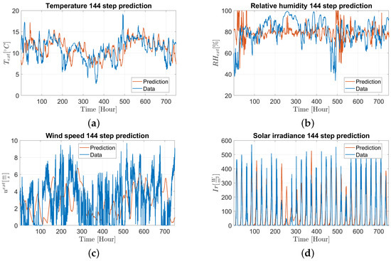
Figure 4.
One-day predictions of all the climate variables considered for short-term climate prediction in the greenhouse. In each graph, the blue line represents the real data measured at the greenhouse, and the red line shows the corresponding model output. (a) Temperature outside the greenhouse ; (b) relative humidity outside the greenhouse ; (c) wind speed outside the greenhouse ; (d) solar irradiance outside the greenhouse .
7.2. Medium-Term Climate Prediction
To test the performance of each of the proposed models, their predictions were compared with simulated data. This was because the real greenhouse climate data were not available at the time of this experiment. The simulated data were generated with the greenhouse climate model. The performance metrics of each model are presented in Table 3 and Table 4, where it can be observed that, in general, the proposed method displayed high prediction error. The high error was expected due to the complexity of climate prediction at this time scale (a sampling time of one day and a prediction horizon of 28 days), the high stochasticity of the involved variables, and the lack of data. This same problem can be observed in Figure 5 and Figure 6. Another detail that can be observed in the tables is that in some cases, a low RMSE was paired with a high MAPE because of the limited amount of data available, resulting in very different samples at the 1-, 14-, and 28-day steps.
Table 3.
Results for the winter data.
Table 4.
Results for the summer data.
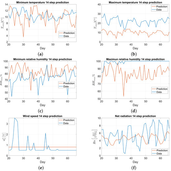
Figure 5.
Fourteen-day predictions of all the climate variables considered for medium-term climate prediction in the greenhouse. The data considered here correspond only to a simulation using the winter data. In each graph, the blue line represents the simulated data, and the red line shows the corresponding predictions. The predictions were output once per day. (a) Minimum greenhouse temperature ; (b) maximum greenhouse temperature ; (c) minimum greenhouse relative humidity ; (d) maximum greenhouse relative humidity ; (e) greenhouse wind speed ; (f) net radiation in the greenhouse .
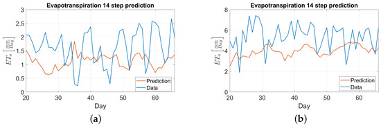
Figure 6.
Comparison between the simulated evapotranspiration data and the corresponding predictions for both winter and summer. The simulated data are represented here by the blue line, and the red line shows the evapotranspiration output of the model. (a) Winter data for evapotranspiration ; (b) summer data for evapotranspiration .
In both datasets, one of the best-performing variables was given the relatively low error, with results generally matching the real values, as shown in Figure 5a. In addition, exhibited one of the highest errors, which corresponded to underestimation, as shown in Figure 5b. A similar result was observed for ; however, the system tended to overestimate the values of this variable, as shown in Figure 5d. led to a similar type of error as that for , with the difference being that the error associated with the former was lower. For wind speed, the constant value was used; this value was obtained with the formula presented in Equation (21). As expected, the corresponding error was one of the highest observed. Figure 5e indicates that for the winter data, the real values approached the minimum wind speed value recommended by the FAO for long periods [27]. For , Figure 5f illustrates that the system effectively simulated the general trend of the actual values but failed to capture some dynamic variability. Finally, Figure 6a,b show that the predicted and real values of displayed similar trends. This result might indicate that enhanced predictions of could improve estimates of and therefore improve the overall performance of the model, as the main objective of this prediction was to obtain future values of . Thus, additional real data should be collected to improve the performance of the models. However, it is possible for the WMS to still function correctly given the corrective nature of the closed-loop MPC.
7.3. Short-Term Management: Window Controller for Climate Control
The proposed climate control scheme was tested in three scenarios using the winter and summer data. The results of the proposed fuzzy controller (MPCF) and the MPC are presented in Table 5 and Figure 7, Figure 8 and Figure 9. The metrics and represent the percentages of time for which the temperature and humidity were in their normal zones, respectively, and and represent the percentages of time for which the temperature and humidity were in their security zones. For both datasets, the system maintained the temperature in the security zone over of the time in contrast to the manual control, for which temperatures were in the security zone only of the time in winter. However, in all cases, the system exhibited problems controlling the humidity of the greenhouse, with the worst performance observed for the winter data. Based on and , the controller performed best when controlling the temperature in the winter case and the humidity in the summer case. Here, it is important to note that based on the local farmer’s experience, there were some cases when the climatic conditions effectively reached a dangerous range of values for temperature and humidity in the real greenhouse. Thus, the crops could survive in these extreme conditions only if they lasted for a short period of time. Additionally, the results reported in Figure 7 and Figure 8 were obtained from a greenhouse model that could not be validated with real data (because of the lack of proper instrumentation inside the greenhouse), so it was not possible to confirm the magnitude of the security zone violations observed. However, despite the problem of model validity, the simulations presented here still provide a guide for how resources could be allocated in these situations.
Table 5.
Climate control results.
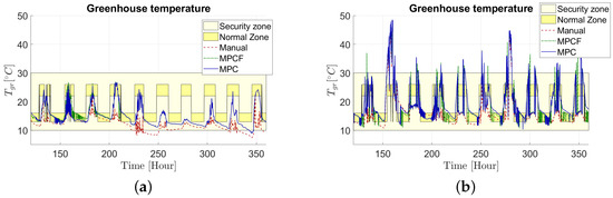
Figure 7.
Temperature obtained inside the greenhouse during the simulations. Both results were compared with the values in the corresponding normal and security zones defined for this climatic variable. These simulation results were obtained using climate data from the winter and summer seasons. (a) Temperature inside the greenhouse when using winter data; (b) temperature inside the greenhouse when using summer data.
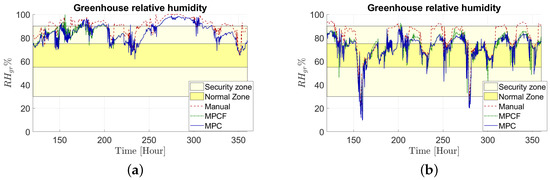
Figure 8.
Relative humidity obtained inside the greenhouse during the simulations. Both results were compared with the values in the corresponding normal and security zones defined for this climatic variable. These simulation results were obtained using climate data from the winter and summer seasons. (a) Relative humidity inside the greenhouse when using winter data; (b) relative humidity inside the greenhouse when using summer data.
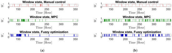
Figure 9.
State of the openness of windows obtained during the simulations. Both graphs correspond to the simulation results obtained when using climate data from the winter and summer seasons. (a) Window state when using winter data; (b) window state when using summer data.
Table 5 shows that both predictive controllers yielded significantly better performance than manual control in all cases, except for changes in window states and temperature in summer, which involved a significant reduction in humidity performance. It can also be observed that the predictive controllers yielded similar results for and in both cases, with the only significant differences observed in the summer. The MPCF performed better in terms of . Additionally, the MPC performed better for , and the MPCF was superior for . This behavior, in conjunction with the previous results, indicated that the MPC sacrificed humidity performance in favor of temperature regulation.
A final observation that can be made is that in both cases, the window state changed more during the summer than the winter, and the MPCF resulted in more window changes than the MPC. From these differences and the performance of the controllers in terms of temperature and humidity, it can be concluded that the system had some difficulties when trying to control humidity using the proposed strategy. Moreover, Figure 7a indicates that the current criteria used to determine day and night conditions might be faulty, and full days might be considered nights if the weather is very cloudy.
7.4. Short-Term Management: Pump and Irrigation Controller for Implementing the EMS
In the simulation, the proposed system could provide 60 L of water for irrigation every 10 min, and 745.699 W of energy was required to operate the pump. The performance of both the manual irrigation approach and the EMS during the simulation is presented in Table 6 and Figure 10 and Figure 11. As shown in Table 6 and Figure 11, both methods consistently provided the desired amount of water or a similar amount while not violating any constraints. The compliance with the programmable constraint is not shown in the results of the tests, because that condition could not be violated, since it was implemented as a correction of the control action for the EMS and is not relevant for manual irrigation. Furthermore, a daily average of five irrigation instances was required to reach the irrigation objective, which coincided with the minimum necessary application. Considering that the system could provide 60 L of irrigation water every 10 min, this result should not be compared to the 18 irrigation instances with manual irrigation, as this number was not related to the greenhouse behavior. Finally, the system required approximately 19.2 battery cycles, which was 0.9 battery cycles less than was used in the manual irrigation case or a hypothetical scenario in which no solar energy was used for pump activation.
Table 6.
EMS performance.
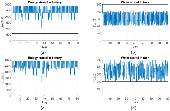
Figure 10.
Energy and water stored in the greenhouse components during the simulations. These resource availability results correspond to the values obtained using climate data from the winter season. Here, the storage limits are represented by black lines. (a) State of energy (SoE) of the battery in the manual irrigation scenario; (b) water volume stored in the tank in the manual irrigation scenario; (c) state of energy (SoE) of the battery in the EMS irrigation scenario; (d) water volume stored in the tank in the EMS irrigation scenario.
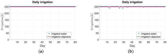
Figure 11.
Daily irrigation performed during the simulation. This daily irrigation volume, represented by the blue points, was compared with the values denoted by the red line, indicating the daily irrigation objective based on medium-term management. (a) Daily irrigation in the manual irrigation scenario; (b) daily irrigation in the EMS irrigation scenario.
7.5. Medium-Term Controller: Implementation of the EWMS
Implementing previous short-term controllers required the reference value of the water volume to be used for irrigation each day , as provided by the EWMS, which operated as a medium-term controller. As mentioned in Section 6, three scenarios for the medium term were studied. In one scenario, half of the greenhouse was irrigated manually, while in the second case, the irrigation was managed by the EWMS. The third scenario combined both previous cases by having each control scheme irrigate one half of the greenhouse but having only the EWMS control the pump.
The results of these simulations are presented in Table 7 and Figure 12 and Figure 13. In both simulations in which the EWMS was used, the system managed to consume less water than manual irrigation while maintaining a high relative yield (over 0.986). Additionally, the EWMS scenarios used significantly less energy than the manual scenario, with the combined scenario consuming slightly less energy than the sum of the two separate scenarios. However, in the case of EWMS irrigation, the system did not achieve all of the daily irrigation objectives. This drawback could have been due to the higher daily objectives compared to those used in the previous test; additionally, the EWMS irrigation case had a comparatively strict minimum tank volume constraint. Still, the system maintained a high relative yield, suggesting that it could adapt to adverse situations. A final observation was that the system did not provide irrigation on some days. This issue may lead to a lack of adoption in communities that usually irrigate daily.
Table 7.
EWMS performance.
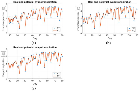
Figure 12.
Comparison between real and potential evapotranspiration and when considering different irrigation scenarios. The real evapotranspiration is indicated by blue points, and potential evapotranspiration is represented by red lines. (a) Real and potential evapotranspiration and in the EWMS case; (b) real and potential evapotranspiration and in the shared manual irrigation case; (c) real and potential evapotranspiration and in the combined irrigation case.
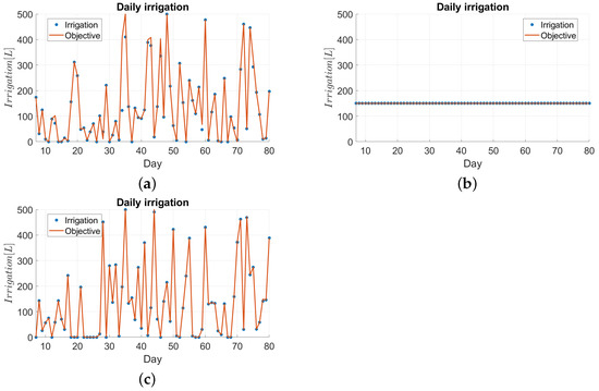
Figure 13.
Comparison between the daily irrigation and the corresponding objective for different irrigation scenarios. The actual irrigation is shown by the blue points, and the corresponding objective is represented by the red lines. (a) Daily irrigation and the corresponding objective for the EWMS irrigation case; (b) daily irrigation and the corresponding objective for the manual irrigation case; (c) daily irrigation and the corresponding objective for the combined irrigation case.
8. Conclusions
The proposed EWMS design presented in this work was based on an MPC for a greenhouse in a Mapuche indigenous community. The greenhouse design was based on previous information regarding greenhouses implemented in the community. The designed system aimed to maximize crop growth while minimizing water use. For this objective, the system was divided into a water management system (short term) and an energy management system (medium term).
The short-term climate prediction was based on the temperature, relative humidity outside the greenhouse, and irradiance dynamics. However, difficulties in predicting wind speed were observed due to the high stochasticity of this variable.
The medium-term climate prediction model, in general, displayed higher errors in its predictions than the short-term model. An important detail could be observed concerning the similarities between the dynamics of net radiation and reference evapotranspiration. This behavior might indicate that the net radiation is the most important factor in estimating evapotranspiration in this environment.
The climate system used only the opening/closing of windows to control the greenhouse microclimate, as it was based on fuzzy MPC. During the simulations, the system managed to maintain the temperature inside the greenhouse in the desired range of values over of the time. On the other hand, the humidity was maintained at the desired value of the time in the best scenario and in the worst case. Another observation was that compared with manual control, the MPCF provided significantly better temperature and humidity control, with a performance difference of over , the exception being the summer temperature, for which the manual control maintained values in the desired zone only more often. Given that this strategy has worked in previous greenhouses, the problem of not complying with the control objectives all the time was likely related to the model’s imprecision; this was further evidenced in the fact that the manual control simulation, which attempted to replicate the farmer’s strategy, displayed the same difficulties during the same periods. The results also indicated that humidity was more challenging to control than temperature when only window openness was controlled.
The simulation for the EMS showed that the proposed controller could successfully provide a daily irrigation volume of 250 L in a real implementation scenario. During this process, the average instances of irrigation in the simulation results were the same as the minimum values required. The system also used solar energy to save 0.9 battery cycles compared to the case in which the farmer’s irrigation pattern was simulated.
The final simulation results showed that the system successfully irrigated crops while reducing water use. In both scenarios that involved the EWMS, the system achieved a relative yield of over 0.986, reflecting good crop development. The proposed controller produced this result despite the low precision of the medium-term predictions and the fact that during one simulation, one of the systems did not achieve the daily irrigation objective because of the high demand for water and the high minimum volume of stored water. Another observation was that, contrary to the daily irrigation performed by the community, the system did not irrigate the greenhouse on certain days. The problem with this is that a system presenting days that lack irrigation could face difficulties in being adopted by the community.
However, before implementing the system, it is recommended to collect more data to improve the greenhouse micro-climate estimation with real data from the greenhouse. It is also recommended to strengthen the medium-term prediction with an emphasis on predicting net radiation, as this is the most important factor for evapotranspiration.
Future research can expand on this work to consider more types of crops in greenhouses. A different possibility is considering a case in which the system irrigates multiple greenhouses simultaneously. Alternatively, excess energy from the system could be sold to the power grid; however, this would sacrifice grid independence. Another possible future objective would be to adapt the system to scarcity situations, as the current system did not consider limitations regarding water extraction.
Author Contributions
Project administration, D.S.; conceptualization, A.E., D.S., S.P. and O.C.; data curation, A.E.; formal analysis, A.E., D.S., C.M. and O.C.; investigation, A.E., D.S., O.C. and J.I.H.; methodology, D.S., C.M. and O.C.; validation, A.E. and J.I.H.; visualization, A.E., D.S., C.M. and S.P.; writing—original draft, A.E., D.S., S.P. and O.C.; writing—review and editing, A.E., D.S., C.M. and J.I.H. All authors have read and agreed to the published version of the manuscript.
Funding
This research was funded by the Instituto Sistemas Complejos de Ingeniería (ISCI) ANID PIA/PUENTE AFB220003; the Solar Energy Research Center (SERC), Chile, ANID/FONDAP/15110019, ANID/FONDECYT 1220507, and ANID/FONDECYT Regular N°1220178; and Basal funding for the Scientific and Technological Center of Excellence, IMPACT, #FB210024. The work of Oscar Cartagena was supported by ANID-PFCHA/Doctorado Nacional/2020-21200709.
Institutional Review Board Statement
Not applicable.
Informed Consent Statement
Not applicable.
Data Availability Statement
The data presented in this study are available on request from the corresponding author.
Conflicts of Interest
The authors declare no conflict of interest.
Abbreviations
The following abbreviations are used in this manuscript:
| WMS | Water management system |
| EMS | Energy management system |
| EWMS | Energy–water management system |
| MPC | Model predictive control |
| MPCF | Model predictive control based on fuzzy optimization |
| TAW | Total available water |
| RAW | Readily available water |
| FAO | Food and Agriculture Organization of the United Nations |
| RMSE | Root mean square error |
| MAPE | Mean absolute percentage error |
Nomenclature
| Daily irrigation objective (m) | |
| Water volume in tank (m) | |
| Volume of irrigated water (m) | |
| Temperature inside the greenhouse (C) | |
| Relative humidity inside the greenhouse | |
| Pump activation decision | |
| Openness of windows | |
| SoE | State of energy (kJ) |
| Temperature outside the greenhouse (C) | |
| Relative humidity outside the greenhouse | |
| Ir | Solar irradiance |
| Wind speed outside the greenhouse | |
| Greenhouse ground temperature (C) | |
| Absolute humidity | |
| t | Sampling time (s) |
| Model sampling time (s) | |
| Heat gain via radiation (W) | |
| Heat via conduction and convection (W) | |
| Heat exchange via air renovation (W) | |
| Heat exchange with ground (W) | |
| Heat loss via evapotranspiration (W) | |
| Air density (kg m) | |
| Soil density (kg m) | |
| Specific heat of dry air (J kgK) | |
| Specific heat of water vapor (J kgK) | |
| Specific heat of the soil (J kgK) | |
| Greenhouse volume (m) | |
| Greenhouse ground area (m) | |
| Greenhouse cover area (m) | |
| Soil temperature measurement depth (m) | |
| Humidity exchange via air renovation (g sm) | |
| Humidity gain via evapotranspiration (g sm) | |
| Wind speed (m s) at height z (m) | |
| Membership function for value z | |
| Inverse membership function for value z | |
| Irrigation caudal (ms) | |
| Battery power required by the system (W) | |
| Power given/received by the battery (W) | |
| Power required by the pump (W) | |
| Power generated by the solar panel (W) | |
| Battery charge efficiency | |
| Battery discharge efficiency | |
| Inversor efficiency | |
| I | Irrigation decision |
| Custom irrigation restriction | |
| BC | Battery cycles |
| Rn | Net radiation in the greenhouse (MJ mDay) |
| A | Planted area (m) |
| Greenhouse absorptivity coefficient | |
| Greenhouse transmissivity coefficient | |
| Absorptivity coefficient of crops and soil | |
| Average wind speed in (m s) at 2 (m) | |
| Average openness | |
| Reference evapotranspiration (mm day) | |
| Potential evapotranspiration (mm day) | |
| Actual evapotranspiration (mm day) | |
| G | Soil heat flux (MJ mDay) |
| Mean saturation vapor pressure (kPa) | |
| Actual saturation vapor pressure (kPa) | |
| Psychrometric constant (kPa C) | |
| Root zone depletion (mm) | |
| TAW | Total available water (mm) |
| RAW | Readily available water (mm) |
| Field capacity | |
| Wilting point | |
| Average water content in soil | |
| Root depth (m) | |
| Total daily irrigation (mm) | |
| DP | Deep percolation (mm) |
| CR | Capillary rise (mm) |
| Irrigation efficiency | |
| Soil porosity | |
| Relative yield | |
| Yield response factor | |
| Mean total radiation in the greenhouse | |
| Saturation vapor pressure–temperature slope (kPa C) |
References
- Karan, E.; Asadi, S.; Mohtar, R.; Baawain, M. Towards the optimization of sustainable food-energy-water systems: A stochastic approach. J. Clean. Prod. 2018, 171, 662–674. [Google Scholar] [CrossRef]
- Chen, C.; Zeng, X.; Yu, L.; Huang, G.; Li, Y. Planning energy-water nexus systems based on a dual risk aversion optimization method under multiple uncertainties. J. Clean. Prod. 2020, 255, 120100. [Google Scholar] [CrossRef]
- Labadie, J.W. Optimal operation of multireservoir systems: State-of-the-art review. J. Water Resour. Plan. Manag. 2004, 130, 93–111. [Google Scholar] [CrossRef]
- Yeh, W.W.G. Reservoir management and operations models: A state-of-the-art review. Water Resour. Res. 1985, 21, 1797–1818. [Google Scholar] [CrossRef]
- Brdys, M.; Grochowski, M.; Gminski, T.; Konarczak, K.; Drewa, M. Hierarchical predictive control of integrated wastewater treatment systems. Control Eng. Pract. 2008, 16, 751–767. [Google Scholar] [CrossRef]
- García, A.M.; Gallagher, J.; McNabola, A.; Poyato, E.C.; Barrios, P.M.; Díaz, J.R. Comparing the environmental and economic impacts of on-or off-grid solar photovoltaics with traditional energy sources for rural irrigation systems. Renew. Energy 2019, 140, 895–904. [Google Scholar] [CrossRef]
- Zavala, V.; López-Luque, R.; Reca, J.; Martínez, J.; Lao, M. Optimal management of a multisector standalone direct pumping photovoltaic irrigation system. Appl. Energy 2020, 260, 114261. [Google Scholar] [CrossRef]
- Yahyaoui, I.; Tadeo, F.; Segatto, M.V. Energy and water management for drip-irrigation of tomatoes in a semi-arid district. Agric. Water Manag. 2017, 183, 4–15. [Google Scholar] [CrossRef]
- Naval, N.; Yusta, J.M. Water-Energy Management for Demand Charges and Energy Cost Optimization of a Pumping Stations System under a Renewable Virtual Power Plant Model. Energies 2020, 13, 2900. [Google Scholar] [CrossRef]
- Golmohamadi, H. Operational scheduling of responsive prosumer farms for day-ahead peak shaving by agricultural demand response aggregators. Int. J. Energy Res. 2021, 45, 938–960. [Google Scholar] [CrossRef]
- Monís, J.I.; López-Luque, R.; Reca, J.; Martínez, J. Multistage Bounded Evolutionary Algorithm to Optimize the Design of Sustainable Photovoltaic (PV) Pumping Irrigation Systems with Storage. Sustainability 2020, 12, 1026. [Google Scholar] [CrossRef]
- Campana, P.E.; Li, H.; Zhang, J.; Zhang, R.; Liu, J.; Yan, J. Economic optimization of photovoltaic water pumping systems for irrigation. Energy Convers. Manag. 2015, 95, 32–41. [Google Scholar] [CrossRef]
- Olcan, C. Multi-objective analytical model for optimal sizing of stand-alone photovoltaic water pumping systems. Energy Convers. Manag. 2015, 100, 358–369. [Google Scholar] [CrossRef]
- Roje, T.; Sáez, D.; Muñoz, C.; Daniele, L. Energy–Water Management System Based on Predictive Control Applied to the Water–Food–Energy Nexus in Rural Communities. Appl. Sci. 2020, 10, 7723. [Google Scholar] [CrossRef]
- Reca, J.; Trillo, C.; Sánchez, J.; Martínez, J.; Valera, D. Optimization model for on-farm irrigation management of Mediterranean greenhouse crops using desalinated and saline water from different sources. Agric. Syst. 2018, 166, 173–183. [Google Scholar] [CrossRef]
- Cartagena, O.; Parra, S.; Muñoz-Carpintero, D.; Marín, L.G.; Sáez, D. Review on Fuzzy and Neural Prediction Interval Modelling for Nonlinear Dynamical Systems. IEEE Access 2021, 9, 23357–23384. [Google Scholar] [CrossRef]
- Camacho, E.F.; Bordons, C. Model Predictive Controllers, 2nd ed.; Springer: London, UK, 2007; p. 405. [Google Scholar] [CrossRef]
- Flores, A.; Saez, D.; Araya, J.; Berenguel, M.; Cipriano, A. Fuzzy predictive control of a solar power plant. IEEE Trans. Fuzzy Syst. 2005, 13, 58–68. [Google Scholar] [CrossRef]
- Ito, K.; Tabei, T. Model Predictive Temperature and Humidity Control of Greenhouse with Ventilation. Procedia Comput. Sci. 2021, 192, 212–221. [Google Scholar] [CrossRef]
- Agmail, W.I.R.; Linker, R.; Arbel, A. Robust Control of Greenhouse Temperature and Humidity. IFAC Proc. Vol. 2009, 42, 138–143. [Google Scholar] [CrossRef]
- Liu, R.; Li, M.; Guzmán, J.; Rodríguez, F. A fast and practical one-dimensional transient model for greenhouse temperature and humidity. Comput. Electron. Agric. 2021, 186, 106186. [Google Scholar] [CrossRef]
- Martínez, D.L.V.; Molina, F.D.; Álvarez, A.J. Ahorro Y Eficiencia EnergéTica en Invernaderos; Instituto para la Diversificación y Ahorro de la Energía: Madrid, Spain, 2008. [Google Scholar]
- Raquel, S.; Mauricio Pérez, A.; Lopez-Cruz, I.; Rojano-Aguilar, A. A model of humidity within a semi-closed greenhouse. Rev. Chapingo Ser. Hortic. 2016, 22, 27–43. [Google Scholar] [CrossRef]
- Stanghellini, C.; de Jong, T. A model of humidity and its applications in a greenhouse. Agric. For. Meteorol. 1995, 76, 129–148. [Google Scholar] [CrossRef]
- Endo, A.; Cartagena, O.; Sáez, D.; Muñoz-Carpintero, D. Predictive Control based on Fuzzy Optimization for Multi-Room HVAC Systems. In Proceedings of the 2020 IEEE International Conference on Fuzzy Systems (FUZZ-IEEE), Glasgow, UK, 19–24 July 2020; pp. 1–8. [Google Scholar] [CrossRef]
- Schwarz, D.; Thompson, A.J.; Kläring, H.P. Guidelines to use tomato in experiments with a controlled environment. Front. Plant Sci. 2014, 5, 625. [Google Scholar] [CrossRef] [PubMed]
- Allen, R.G.; Pereira, L.S.; Raes, D.; Smith, M. Crop evapotranspiration-Guidelines for computing crop water requirements-FAO Irrigation and drainage paper 56. Fao Rome 1998, 300, D05109. [Google Scholar]
- Marín, L.G.; Sumner, M.; Muñoz-Carpintero, D.; Köbrich, D.; Pholboon, S.; Sáez, D.; Núñez, A. Hierarchical Energy Management System for Microgrid Operation Based on Robust Model Predictive Control. Energies 2019, 12, 4453. [Google Scholar] [CrossRef]


Disclaimer/Publisher’s Note: The statements, opinions and data contained in all publications are solely those of the individual author(s) and contributor(s) and not of MDPI and/or the editor(s). MDPI and/or the editor(s) disclaim responsibility for any injury to people or property resulting from any ideas, methods, instructions or products referred to in the content. |
© 2023 by the authors. Licensee MDPI, Basel, Switzerland. This article is an open access article distributed under the terms and conditions of the Creative Commons Attribution (CC BY) license (https://creativecommons.org/licenses/by/4.0/).