Predicting Reservoir Petrophysical Geobodies from Seismic Data Using Enhanced Extended Elastic Impedance Inversion

Abstract

The study aims to implement a high-resolution Extended Elastic Impedance (EEI) inversion to estimate the petrophysical properties (e.g., porosity, saturation and volume of shale) from seismic and well log data. The inversion resolves the pitfall of basic EEI inversion in inverting below-tuning seismic data. The resolution, dimensionality and absolute value of basic EEI inversion are improved by employing stochastic perturbation constrained by integrated energy spectra attribute in a Bayesian Markov Chain Monte Carlo framework. A general regression neural network (GRNN) is trained to learn and memorize the relationship between the stochastically perturbed EEI and the associated well petrophysical log data. The trained GRNN is then used to predict the petrophysical properties of any given stochastic processed EEI. The proposed inversion was successfully conducted to invert the volume of shale, porosity and water saturation of a 4.0 m thick gas sand reservoir in Sarawak Basin, Malaysia. The three petrophysical geobodies were successfully built using the discovery wells cut-off values, showing that the inverted petrophysical properties satisfactorily reconstruct the well petrophysical logs with sufficient resolution and an accurate absolute value at the well site and are laterally conformable with seismic data. Inversion provides reliable petrophysical properties prediction that potentially helps further reservoir development for the study field.

1. Introduction

One critical issue in petroleum industry economics is an estimation of hydrocarbon volume. The existence of hydrocarbons is determined by the petrophysical properties of the reservoir. Petrophysical data sets are key information during the production phase and are needed for determining the recovery factor after long-term production of a reservoir. Advanced reservoir study, e.g., reservoir simulation, used petrophysical data as a basis of study [1,2]. Such process and study need reliable petrophysical data from which the hydrocarbon reservoir will be characterized in detail. The reservoir distribution that includes the reservoir thickness, areal extent and spatial variability needs to be delineated, and the hydrocarbon volume has to be quantitatively estimated. It is important to accurately estimate the reservoir’s petrophysical properties to support the reservoir characterization.

The areal extent of the reservoir is determined from seismic data. A comprehensive reservoir description is achieved through the integration of the well petrophysical properties log and three-dimensional seismic data. Such integration is needed in order to understand, as much detail as possible, the deployment of the rock petrophysical parameters of the reservoir.

Seismic inversion is one method to integrate the well log and seismic data. Seismic inversion aims to transform seismic data into the rock and fluid properties of the earth. Acoustic impedance inversion is the most basic seismic inversion [3]. It calculates the acoustic impedance (product of compressional velocity and density) of the earth layer from which the geological properties of the earth can be predicted. With the proper use of acoustic impedance and/or integration with other methods, acoustic impedance inversion can be conducted for advanced reservoir characterization, such as reservoir properties distribution and discrimination between lithology, porosity and fluid effects. Recently, Anees et al. [4] used advanced constrained sparse spike inversion (CSSI) to identify the spatial sand ratio distribution of a tight sand gas reservoir. They successfully distinguished the tight sand from coal and mudstone facies by analyzing the acoustic impedance volume inverted by CSSI. Using further analysis, they also successfully interpreted the presence of the environment of depositional, i.e., thick fluvial braided channels and braided bars where the tight sandstone is accumulated and the inter-distributary channels where the mudstone facies are present. Ashraf et al. [5] integrated petrophysical, geostatistical analysis and rock physics with CSSI to characterize the heterogeneity of a clastic reservoir through the inverted acoustic impedance volume analysis. They showed that the integration was able to precisely characterize the reservoir parameter within the zone of interest shown by the well delineation of the lithofacies distribution and its heterogeneity. However, Ashraf et al. [5] suggested that to invert the acoustic impedance, density and Vp/Vs ratio using elastic impedance inversion, which is capable of extracting numerous petroelastic parameters that are evidently vital from stratigraphic and sedimentological perspectives.

Elastic impedance (EI) inversion aims to invert not only acoustic but also elastic characteristics of the earth layer. Different from acoustic impedance inversion, which uses single reflection (normal or zero angle incidence reflection), elastic impedance inversion uses either normal (zero angle incidence) or non-normal (non-zero angle incidence) reflection seismic data to characterize the earth layer geology. EI inversion showed that the zero angle incidences seismic signature respond the acoustic properties and the non-zero angle incidences signature respond the elastic properties from where the earth lithology and fluid information can be characterized. There are two ways to collect or gather the non-zero angle incidence seismic data from those that are common azimuth and variable azimuth. In common azimuth, the seismic data is gathered in a certain straight line (certain azimuth). The seismic data is stacked based on various offsets or angles of incidence, and the famous format is near, mid and far stacked seismic data. Differently, in variable azimuth, seismic data is stacked for a certain angle of incidence in various azimuthal directions and commonly labeled as 0°, …, 360°. Common azimuth data, well known as partial or pre-stack data, is widely used for reservoir lithological and fluid inversion, while variable azimuth data is used for characterizing the anisotropic behavior of the reservoir. When seismic data is rich in azimuths, it can be used by an anisotropic method to estimate the earth’s anisotropy parameters [6]. Anisotropy analysis, such as vertical and horizontal transverse isotropy (VTI/HTI), can be conducted with amplitude versus azimuth (AVAz) reflectivity and azimuthal inversion. Recently, Li et al. [7] successfully inverted quantitatively the fracture weakness parameter from a vertically fractured reservoir. They predicted the second Fourier coefficient and the azimuth of the symmetry axis of the inverted azimuthal EI datasets and combined them to estimate the fracture weaknesses. They found that the proposed inversion is stable and reliable when the azimuth of the symmetry axis deviates less than 30°. They explained that the proposed inversion is dependent on the correctness of the constructed anisotropic rock physical model; therefore, the reliability of the inversion remains questioned.

Elastic impedance inversion in the common azimuth data domain is also widely used in the industry. While the azimuthal inversion is conducted with AVAz (amplitude versus azimuth) reflectivity, the EI inversion in common azimuth is conducted with AVA (amplitude variation with angle) or AVO (amplitude versus offset) reflectivity. The elastic properties are commonly estimated by solving simultaneously the AVO equation for a given set of angle-stacked data. The main result of the inversion is commonly compressional impedance, shear impedance and density. Compressional velocity, shear velocity and Poisson’s ratio are usually inverted as an additional result. Recently, Adesanya et al. [8] used a simultaneous inversion from commercial software to delineate the hydrocarbon reservoir from a subtle seismic feature that failed to be conducted by traditional seismic inversion. Utilizing four wells and five stacked seismic data, they successfully delineated the reservoir well validated by a blind well test. They show the effectivity of the inversion from the volume of the inverted compressional-impedance, shear-impedance, density, near and far-far lambda-rho, mu-rho and Poisson’s-ratio that reveal vertical and lateral continuity of the reservoir.

Although the non-zero angle incidence seismic data is believed to bring various elastic properties information, in practice, the AVO equation limits the applicable range of the angle of incidence and when the angle of incidence is very large, it leads the reflectivity value to exceeds one which conflicts with real seismic data. Whitcombe et al. [9] proposed to rotate the AVO equation such that the square sinus of the incidence angle is equal to the tangent of the angle of rotation. The elastic reflectivity is, consequently, not only a function of the incidence angle but also the rotation angle and called extended elastic impedance (EEI) reflectivity. The angle of rotation changes between −90° and 90°, extending the elastic impedance for any given angle of incidence. The rotation angle that corresponds to the maximum cross correlation between the elastic (or any physical) parameter and EEI and is called the optimum of angle of rotation and can be used to predict the parameter from any given EI at a certain angle of incidence set. Sharifi et al. [10] conducted a feasibility study to see if EEI spectrum variation exhibits any sensitivity to hydrocarbon reservoir geomechanical parameters. They obtained the optimum rotation angle by cross correlating the static and dynamic moduli of the reservoir rock with the corresponding calculated EEI from different rotation angles and generated 3D reflectivity EEI for every obtained optimum angle of rotation. The geomechanical parameter cubes are generated by performing model-based inversion applied to the 3D EEI reflectivity. Sharifi et al. [10] claimed that their proposed inversion result was in comparable accuracy with those of simultaneous inversion, with validation from the blind-well test, and, therefore, it can bring significant progress in the future. To attain more accurate results, Sharifi et al. [10] recommended conducting a feasibility step to take into account the uncertainty of the empirical angle of rotation and the use of other seismic analysis along with EEI analysis.

Aleardi [11] demonstrated the use of EEI to directly estimate the petrophysical properties (i.e., porosity, water saturation and shaliness) from seismic data of a clastic gas reservoir. They determined the optimum angle of rotation for each petrophysical parameter through a petrophysical analysis. The volume of intercept and gradient impedance are derived from seismic data volume using simultaneous inversion and projected to the optimum angle of rotation corresponding to the petrophysical parameter as predicted petrophysical properties. They showed that the inverted petrophysical values revealed a proper match at the blind well location. In conclusion, EEI inversion is effective for lithology and fluid prediction in clastic reservoirs. The result of inversion can be beneficial for static reservoir model building, volumetric calculation and determination of new potential drilling locations. For the successful application of EEI in petrophysical prediction, Aleardi [11] reminded us that seismic processing should ensure that the reservoir amplitude versus angle (AVA) responses are preserved in the seismic data. It was also recommended to use a more sophisticated inversion strategy (based on tailored rock-physic models) to use the EEI for predicting petrophysical properties from the different geologic scenarios.

This paper proposes an enhancement of EEI inversion in order to make it able to invert petrophysical properties from subtle seismic data. Stochastic and neural network techniques will be used to improve the vertical resolution, unity and absolute value of the EEI inversion result. The stochastic process will build EEI reflectivity models by perturbing the basic inverted EEI reflectivity with constraints from the basic inverted EEI signature and petrophysical log data. The constraints take the role of guiding the perturbation to produce EEI models that obey both the EEI signature and well petrophysical log data. The neural network aims to learn and memorize the relationship between the perturbed EEI models and the well petrophysical logs, which are used for predicting the petrophysical properties away from well locations. The proposed method is implemented to predict porosity, the volume of shale and water saturation from a gas field composed of thin sand–shale sequences in the Sarawak Basin, Malaysia.

2. Data and Methods

2.1. Data

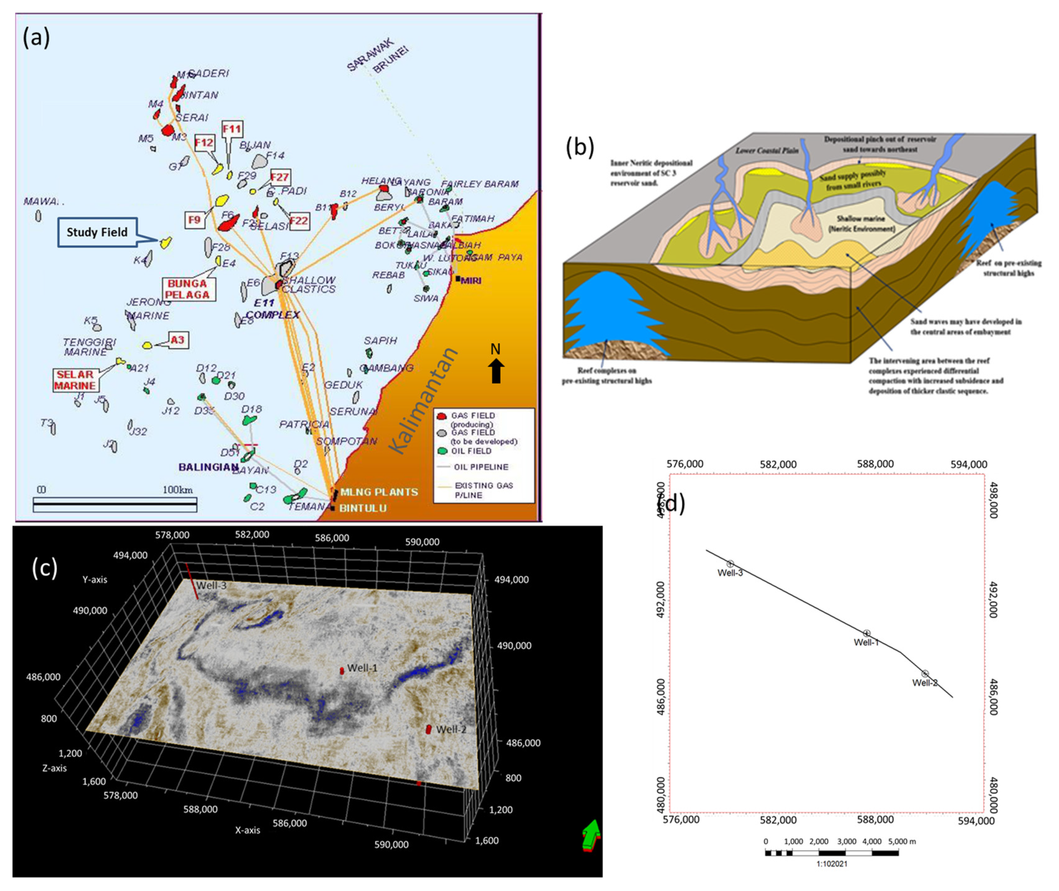
2.1.1. Study Field Geological Setting

The study field is located about 200 km from Bintulu, in a water depth of 79.0 m, offshore in the Sarawak Basin of Malaysia (Figure 1a). Complex interaction and compressional among the continental Philippine tectonic plate to the Northeast, the oceanic Indian continental Australian tectonic plate to the South and Southwest and the oceanic Pacific tectonic plate to the East during the Cenozoic Era shaped the present-day tectonic of the studied field [12].

Interpretation of seismic data indicates that a reservoir sand layer pinched out updip, and the effects of both structural and stratigraphic elements have contributed to the formation of a combination trap structure. The reservoir sand was deposited in the shallow marine inner neritic environment (Figure 1b). It is an intervened area between reef complexes that have experienced differential compaction due to increased subsidence and deposition of a thicker clastic sequence.

2.1.2. Study Field Petroleum System

Major hydrocarbon occurrence in the studied field is illustrated in a generalized stratigraphy in Figure 2a. According to Madon and Abolins [13], the main hydrocarbons at play in this area are Oligocene-Early Miocene Cycles 1 and 2 coastal plain sands, sealed by intra-formational shales and trapped in wrench related anticline. The identified plays are clastic reservoirs of the late Miocene to Early Pliocene age. The abundance of gas in the study field was suggested due to factors of humic and/or gas-prone marine source rocks in the Cycle 1 and 2 kitchen areas and the contrasting maturation and trap-timing histories. Sedimentation in Cycle 1 (or Cycle 2) to Cycle 8 is cut by the NE–SW strike faults that, for most of them, are not sealed and have very deep roots until sourced at the depth of Cycle 1 and Cycle 2 level. The faults act as major paths of hydrocarbon migration from the source rock to the main reservoir SC3 in the studied field (Figure 2b).

The hydrocarbon accumulation is identified by high amplitude anomalies in the maximum trough amplitude, as shown in the seismic section passing three available wells (Figure 2c). Abrupt changes and structural conformability of SC3 seismic anomalies directly indicate the hydrocarbon occurrence. The interval velocity at the SC3 level is about 2400 m/s, so the tuning thickness here is about 12 m. Since the average thickness of SC3 sand is around 18 m to 28 m, the top and bottom reflectors of the SC3 reservoir can be tracked based on full stacking seismic data. However, due to the strong AVO impacts, the spill point location and the fluid variation inside the reservoir cannot be defined accurately.

The three available wells encountered six reservoir layers above and below the SC3 pay with variable thicknesses. SC3A is one of the six encountered reservoirs. The 1140 sand is indicated as a non-hydrocarbon reservoir. SC3 reservoir sand has sufficient thickness, therefore, is distinct and shows good seismic amplitude anomaly (Figure 2c), whereas the SC3A sand and other discovered pays are thin. The structure is quite subtle in nature, with very small relief, which might have formed due to differential compaction. The above SC3 reservoir horizons are very character consistent and continuous over the field 3D survey. However, the below SC3 horizons are relatively weak and discontinuous.

2.1.3. Data for Inversion

This article uses partial (near and far) stacked seismic and three available well-log datasets from the studied field. Figure 3a,b consecutively show the near and far seismic section that passes through the three available wells, Well one, Well two and Well three, with Gamma Ray log from each well inserted. The acquired seismic dataset quality is considered good as the structural and stratigraphic features in this field of study can be seen clearly from the 3D seismic data. The seismic dataset over the gas reservoir demonstrates a very strong AVO anomaly (Figure 3a,b). The dominant frequency at the major reservoir zone from the full stacking volume is around 35 Hz to 40 Hz, but the seismic wavelet shows mixed phase characteristics.

Based on the internal report, the seismic data are tied well with the log data and allow for the identification of the key seismic events. Figure 3c illustrates the seismic-to-well tie process for Well one. The seismic wavelet was extracted along the well bore by using an autocorrelation algorithm and applied with the Ricker wavelet together to produce the synthetics. The synthetics’ ties to the seismic are generally good. The reliable match was obtained by manual adjustment of the synthetic to the seismic data using the check shots in Well one. The clear tie was obtained using the reflectivity series of the well and zero phase wavelet. The best synthetic tie was obtained by fixing the reflectivity series calculated from the sonic and density logs with the check shots and extracting the seismic wavelet from the seismic. The extracted wavelets showed that the phase of the wavelet was near zero phases, and no lag was needed to obtain the match in wells. The synthetics were generated from full stack migration seismic volume. Most of them have a good match with calculated borehole reflectivity impedance. The synthetic seismogram yields an understanding of the influence of variant reservoir properties, such as vertical reservoir distribution, porosity, lithology and fluid saturation on the seismic wavelet.

The three wells encountered about 20 m of total net hydrocarbon sand in the thick SC3 reservoir. The net thickness varies from 17.5 m to about 24.5 m, with porosity ranging from 24% to 30%. The net thickness of thin SC3A sand ranges from 4 m to 12 m, with porosity in the range of 18 to 23%. Porosities are mainly intergranular in nature. The SC3A sandstone reservoir is thin, with only 4.0 m of the total thickness.

Three petrophysical logs (porosity, water saturation and volume of shale) from three available wells (Figure 4) are involved in the inversion. Porosity, water saturation and volume of shale from Well one are used for calibration, whereas the rest (from Well two and Well –three) are used for a blind test.

2.2. Methodology

This article proposes a petrophysical properties prediction by enhancing the traditional EEI inversion with the stochastic process and neural network techniques. The workflow is figured in Figure 5.

EEI inversion is implemented for the first estimate of petrophysical properties. The result is then enhanced in terms of resolution and dimensionality using a stochastic process. The generalized regression neural network is trained to learn the relationship between the enhanced petrophysical EEI with the petrophysical log data. The trained GRNN is then used to predict the volumetric petrophysical properties, as the inversion final result, from where the Geobody of the reservoir is extracted and delineated.

2.2.1. Extended Elastic Impedance (EEI) Inversion

The EEI inversion is introduced by Whitcombe et al. [9], which is an extended concept of elastic impedance (EI) inversion introduced by Connolly [14]. The EEI is formulated as:

$$\mathrm{EEI}(\mathsf{\chi })=\mathrm{A}{\mathrm{I}}_0\left[{\frac{AI}{A{I}_0}}^{\cos \left(\chi \right)}{\frac{GI}{G{I}_0}}^{\sin \left(\chi \right)}\right],$$

(1)

where χ is the amplitude versus offset (AVO) rotation angle, AI is acoustic impedance, GI is gradient impedance and AI₀ and GI₀ are, consecutively, normalized AI and GI [9].

The EEI formulation Equation (1) suggests that the EEI values for different χ angles at any given partial seismic data can be inverted once the AI and GI values are obtained. In this paper, AI and GI are obtained by solving simultaneously the two-term AVO equation [15] for two (near and far) angles of stacks. The pre-stack seismic data simultaneous inversion approach [16] is used to calculate AI and GI.

The estimated petrophysical properties associated with EEI (EEI petrophysics) are obtained by correlating Equation (1) with the targeted petrophysical log for certain optimum χ angles. The optimum χ is obtained at the well site location by simulating Equation (1) for scanned χ angles from −90 to +90 degrees. The EEI with the highest correlation with the petrophysical log is chosen as the estimated petrophysical properties, and the associated χ angle is chosen as the optimum χ. The optimum χ then can be used to estimate the petrophysical properties for any other given calculated AI and GI entire seismic data volume.

2.2.2. Stochastic Process

This article proposes to enhance the resolution, as well as the petrophysical absolute value prediction, of the traditional EEI inversion by applying a stochastic process to the traditional EEI inversion result. The process assumes that the traditional EEI inversion result is still contained by seismic wavelet and therefore has an insufficient frequency band (low in resolution). The assumption implies that the EEI inversion result is assumed to be a convolution between EEI reflectivity and EEI wavelet. The stochastic process aims to modify the EEI reflectivity such that it has frequency as a petrophysical log frequency and, at the same time, when convolving with EEI wavelet, has a similar signature to the inverted traditional EEI. To achieve the goal, a Bayesian Monte Carlo simulation is employed to simulate the EEI reflectivity and select the best model as the inversion result. The simulation is conducted in the probability density function domain and formulated as:

$$\mathrm{P}\left(EE{I}_{\mathrm{pr}}|EEI\right)=\frac{\mathrm{P}\left(EEI|EE{I}_{\mathrm{pr}}\right)\times \mathrm{P}\left(EE{I}_{\mathrm{pr}}\right)}{\mathrm{P}\left(EEI\right)},$$

(2)

where $\mathrm{P}\left(EE{I}_{\mathrm{pr}}|EEI\right)$ is the posterior probability or the result of simulation which informs the best solution, $\mathrm{P}\left(EEI|EE{I}_{\mathrm{pr}}\right)$ is the likelihood between prior and observed EEI. $\mathrm{P}\left(EE{I}_{\mathrm{pr}}\right)$is the probability of the prior model $EE{I}_{\mathrm{pr}}$, and $\mathrm{P}\left(EEI\right)$ is the probability of the observed EEI.

The EEI prior model is populated or perturbed by randomly modifying the two consecutive reflectors space (bed thickness in the earth layer model) of the observed EEI. The perturbation is constrained by seismic thickness criteria, i.e., maximum amplitude [17], tuning frequency [18], maximum amplitude weighted integrated energy spectra [19] and low and high-frequency models derived from petrophysical log data. A random noise of up to 20% can be added to the EEI prior model. The populated EEI prior model is then iteratively selected to be the EEI posterior model (the result of inversion) following the Markov Chain rule.

2.2.3. Neural Network Modelling

This article uses the generalized regression neural network (GRNN) to learn and memorize the relationship between the EEI posterior model and the petrophysical properties log at the well location in order to enhance and ensure the accuracy of the petrophysical properties prediction given the seismic data volume where no well log data is available. GRNN is a radial basis neural network that consists of four layers, i.e., input, pattern, summation and output layers [20]. The GRNN is trained with the posterior model EEI_po as training input and the petrophysical log P_log as training target with the following scheme:

$$\overline{{\mathrm{P}}_{\log }}\left(EE{I}_{\mathrm{po}}\right)=\frac{{\sum }_{\mathrm{i}=1}^{\mathrm{n}}{\mathrm{P}}_{{\log }_{\mathrm{i}}}{ \mathrm{e}}^{\left(-\frac{{\mathrm{D}}_{\mathrm{i}}^2}{2{\mathsf{\sigma }}^2}\right)}}{{\sum }_{\mathrm{i}=1}^{\mathrm{n}}{\mathrm{e}}^{\left(-\frac{{\mathrm{D}}_{\mathrm{i}}^2}{2{\mathsf{\sigma }}^2}\right)}},$$

(3)

where $\overline{{\mathrm{P}}_{\log }}$ is the estimated petrophysical log for given posterior model EEI_po. i is sample index, n is number of samples, σ is sample smoothing factor or spread that is optimized by the trial-and-error process. ${\mathrm{e}}^{\left(-\frac{{\mathrm{D}}_{\mathrm{i}}^2}{2{\mathsf{\sigma }}^2}\right)}$ has a role of the GRNN activation function. ${\mathrm{D}}_{\mathrm{i}}^2$ is the squared distance between the samples and the point of prediction.

The training is conducted iteratively until the mean-squared error between estimated petrophysical, $\overline{{\mathrm{P}}_{\log }}$, and targeted petrophysical log, P_log, is minimum. The smoothing factor δ is the only adjustable factor to control the performance of the simulation. It has to be defined (trial and error) before training. A smoothing factor value that gives the highest correlation and smallest error between the actual and predicted value should be obtained to optimize the GRNN model. Theoretically, when the smoothing factor value is much bigger than zero, smooth interpolation values between the actual values will be produced. The smoothing factor can be allowed to be very small (approaches zero) in order to fit the actual data and allows for high-order curves [20].

GRNN modeling can be conducted in the MATLAB system using the newgrnn built-in function. Model training can be conducted with syntax [21]:

net = newgrnn(P,T,spread),

(4)

where ‘net’ is the GRNN model being built, ‘P’ is input vectors, ‘T’ is target vectors and ‘spread’ is the smoothing factor.

And model testing can be conducted using syntax:

T′ = net(P′),

(5)

where ‘T’ is the prediction vectors and ‘P’ is the new input vectors.

The smoothing factor ‘spread’, as well as the GRNN model ‘net’, can be optimized by manually simulating the value of ‘spread’. The optimized model is associated with the ‘spread’ value that gives the smallest error between the predicted vectors ‘T′’ and the target vectors ‘T’.

2.2.4. Petrophysical Prediction

The petrophysical properties prediction from any perturbed EEI away from the well is conducted using the trained GRNN model by substituting the perturbed EEI into the$EE{I}_{\mathrm{po}}$, with smoothing factor δ value that was optimized during the training process. In the MATLAB system, the training of GRNN for the petrophysical prediction can be conducted by substituting the well site perturbed EEI into ‘P’, the petrophysical log into ‘T’, and the δ into ‘spread’ in Equation (4). After the model is optimized, through various δ values simulation, petrophysical properties can be predicted using Equation (5) by substituting the new perturbed EEI into ‘P′’. The predicted petrophysical properties are represented by ‘T′’.

2.2.5. Geobody Generation

Seismic reservoir characterization is commonly conducted based on the integration of reservoir properties in a 3D geobody/geocellular model [22]. Geobody is a geological modeling terminology to describe the geological elements in a reservoir. As a result of the depositional environment, these elements are often distinctive, giving insight into the reservoir architecture. Geobody can be delineated or generated through facies modeling [23] and spectral decomposition volume attributes analysis [24]. Ashraf et al. [23] used an interactive approach of petrophysical, mineral composition, well-log facies and horizon attribute analyses, unsupervised vector quantifier artificial neural network and sequential indicator simulation to model the reservoir facies. They successfully generated a geobody that delineates a fluvial fan-delta sedimentary system. The reservoir sand depositional environment, sand distribution and thinly laminated beds of fine-grained black shale and lime muddy siltstones are identified very well. Whereas Olaniyi et.al [24] successfully identified channels and defined the reservoir architecture by analyzing the 3D volume of dominant frequencies from spectral decomposition attributes.

In this article, geobodies are generated using cutoff analysis. The geobody of reservoirs is delineated by three-dimensional mapping of the extracted petrophysical value that was selected using the discovery well cutoff value. Expectedly, the generated quantitative petrophysical geobody is able to not only spatially delineate the reservoir but also help the reservoir development, e.g., reservoir modeling and reservoir simulation.

3. Results

3.1. EEI Petrophysic Optimum χ Angle

The inversion for porosity, water saturation and the volume of shale in the field was conducted using the near and far seismic and Well one log data as input. The AI and GI at Well one sites are, firstly, calculated by solving a two term AVO equation [15] for the given Well one near and far seismic traces. The optimum χ angle for each porosity, water saturation and volume of shale are obtained using EEI formulation, Equation (1), for χ angle scanned from −90 to +90 degrees. The correlation coefficient between the logarithmic of EEI, which is the estimated petrophysical property, and the corresponding petrophysical log are calculated for every simulated χ angle value and cross-plotted. Figure 6 shows the correlation coefficient and χ angle cross plot for the three petrophysical parameters under investigation.

The cross-plot in Figure 6 shows a low correlation coefficient for all porosity, water saturation and the volume of shale. For a χ angle equal to −57°, the porosity and volume of shale show the strongest positive correlation with ln (EEI). Differently, the water saturation gives the highest correlation with ln (EEI) for the χ angle equal to −54°. Although small in value, the three-correlation coefficient and the χ angle cross plots show a maximum/minimum peak which implies that each volume of shale, porosity and water saturation from Well one has a unique relationship with the EEI of the study field. The χ angle −57° is a predictor for porosity and the volume of shale, whereas –54° is a predictor for water saturation in the study field. The low correlation coefficients may indicate that predicting porosity, water saturation and volume of shale using EEI is less reliable for the study field.

3.2. Stochastic Petrophysical EEI Model Enhancement

The traditionally inverted petrophysical is then enhanced by a stochastic process in order to improve the resolution and dimensionality, as illustrated in Figure 7; porosity prediction is taken, for example. The stochastic process aims to build an equiprobable EEI porosity reflectivity model that is as close as possible to porosity log reflectivity (Figure 7a) and EEI porosity signature as close as possible to the observed EEI porosity signature (Figure 7b).

Figure 7c shows the minimum and maximum attribute extracted from the EEI porosity signature (Figure 7b) that is used for the initial prior EEI porosity reflectivity model. Figure 7d shows the applied wavelet that is extracted statistically from the EEI porosity signature (Figure 7b).

Random perturbation is applied to the EEI porosity model (Figure 7c) to produce the equiprobable prior EEI porosity reflectivity model (Figure 7e). In this example, 50 prior models are generated. There is no limitation on how many models have to be generated. One clue is that the number of models should enable the simulation to achieve its global minima. The 50 equiprobable EEI porosity signatures (Figure 7f) are then generated by convolving every prior EEI porosity reflectivity model in Figure 7e with applied wavelet, Figure 7d.

From the 50 EEI porosity signature model, Bayesian simulation is then conducted to select one prior model that possesses the best match with the observed EEI porosity signature. The selected EEI porosity signature prior model is then defined as the EEI porosity posterior model, which is the solution of the simulation. The EEI porosity reflectivity prior model associated with the selected EEI porosity signature model is defined as the posterior EEI porosity reflectivity model, which when it is transformed into the impedance form, will be closer to the porosity log. In this example, the posterior EEI porosity signature and posterior EEI porosity reflectivity are overlaid, consecutively, on prior EEI porosity signature models (Figure 7f) and prior EEI porosity reflectivity models (Figure 7e) in thick blue curves.

3.3. GRNN Model

This article uses MATLAB’s built-in newgrnn function to build the GRNN model for porosity, water saturation and the volume of shale prediction for the study of seismic and well log datasets. The GRNN model is trained and optimized using Well one near and far seismic date traces as the training input and petrophysical log (porosity, water saturation and the volume of shale) as the training target. A total of 188 samples covering the zone of interest are selected to conduct the training. The GRNN smoothing factor (identified as spread in the newgrnn function syntax) is estimated by taking the absolute mean of the difference between the inverted EEI for each of the petrophysical data (porosity, water saturation and the volume of shale) and its mean. The smoothing factor of 4e-15, 6e-15 and 4e-15 is obtained, correspondingly, for porosity, water saturation and the volume of shale.

To validate the estimated smoothing factors, experimental simulation is conducted to take the R-squared (R²) value between the estimated petrophysical properties versus the targeted log for smoothing factors between zero and two, including the guest smoothing factors. Figure 8 shows the diagram of a newgrnn training that was conducted to determine one GRNN model for the petrophysical properties from one inverted EEI with one smoothing factor in the selected range. Figure 8 informs that there are four layers and 191 neurons, in total, involved during a sort of training.

Figure 9 shows a comparison between predicted petrophysical properties and their associated log target for various values of the smoothing factor (σ). The smoothing factor of low, middle and high is taken for simulation. Figure 9 shows how the accuracy R² varies with the changing of a smoothing factor value. Comparing the R² given by the three smoothing factors, it indicates that the porosity prediction has maximum R² at the middle smoothing factor value, while water saturation and the volume of shale predictions achieve their maximum R² at low and high smoothing factor values.

To obtain the optimum smoothing factor, a denser simulation is conducted for the smoothing factor values between zero and two, and the accuracy R² and smoothing factor is then cross plotted. Figure 10 shows the cross plot of R² for the estimated petrophysical properties (porosity, water saturation and the volume of shale) with the scanned smoothing factor between zero and two. As shown in Figure 10, the maximum R² for porosity, water saturation and the volume of shale is, respectively, about, 0.81 (achieved at smoothing factor 1.1), 0.9 and 0.8 (achieved at smoothing factor in 0 to 0.2 range). The given R²s indicate the governed GRNN models for the three petrophysical properties are well trained [25]. The R² curves, which are obtained by comparing the GRNN simulation output and the training target, show that the trainings converge within the range of the applied smoothing factor as the R² approaches one [20].

3.4. Porosity Prediction

3.4.1. Well-1 Site Porosity Prediction

Figure 11 illustrates the inversion of porosity at the Well one location. There are three anomalies in the well log, i.e., thick SC3 and thin SC3A gas sand and water sand, just below the SC3A. Those three anomalies are represented by three high values of porosity (Figure 11a). The far seismic trace (Figure 11c) shows a strong AVO anomaly compared to the near seismic trace (Figure 11b), especially for shallower thick reservoir SC3. Although small, the anomaly of the deeper thin reservoir SC3A is recognizable. Figure 11d shows the traditional inverted EEI porosity. It is shown that the traditional EEI porosity is negatively correlated with the porosity log, and the absolute value is not recovered yet. The three targeted porous sand are identified by the traditional inverted EEI porosity; however the resolution is poor.

Figure 11e shows the proposed inverted EEI porosity (blue curve), resulting from applying stochastic process and GRNN to the traditionally inverted EEI porosity (Figure 11d), overlaid by the targeted porosity log (red curve). As shown in Figure 11e, the porosity prediction is significantly improved. The match between inverted EEI porosity and targeted porosity log is improved. The deeper thin SC3A reservoir sand and the water sand are captured. The porosity of all porous sands is estimated closely to targeted log data. The mismatch between predicted and targeted porosity at around 1100–1200 ms is suggested due to strong seismic amplitude data that is not supported by sufficient porosity data measured at well logging, therefore, making the inversion overestimate the porosity value at that zone.

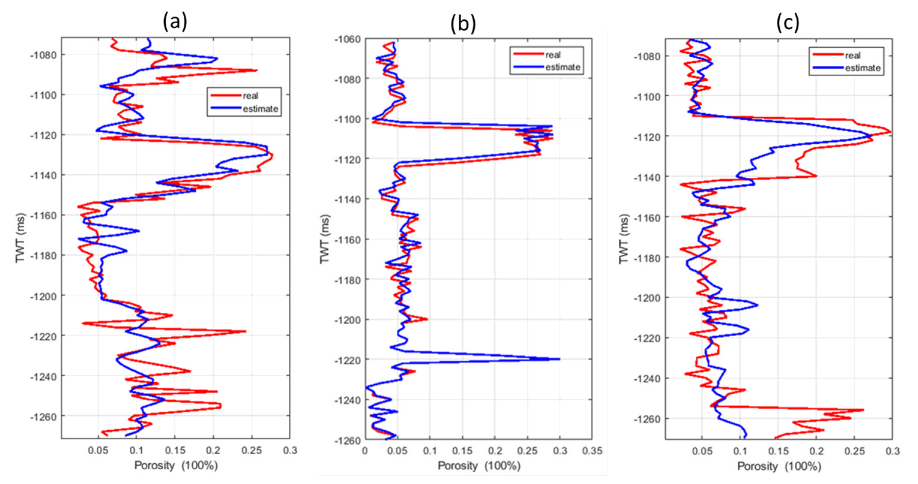
3.4.2. Inversion Result Validation

Figure 12 compares the proposed EEI porosity predictions (in blue) with the well’s porosity log curve (in red). Well three (Figure 12b) is used as a control or calibration; Well two (Figure 12c) and Well three (Figure 12a) are blind. Both predicted, and log porosity is plotted with a five point moving average smoothed filter. The quality of this prediction is acceptably good, with the predicted porosity curve lying closely with the well porosity log.

The cross plot of the estimated EEI porosity against the targeted porosity log for the three wells is shown in Figure 13. The cross plot for Well one (Figure 13b) gives an R-squared factor (R²) of 0.81, while both the cross plot for blind Well three (Figure 13a) and Well two (Figure 13c) give R² of, respectively, 0.67 and 0.72. The R² values inform that more than half of the predicted porosity in this inversion can explain the targeted or measured porosity [26]. The R² of 0.81, 0.72 and 0.67 indicate that the porosity estimation is performing well at both control and blind well location [25].

3.5. Water Saturation and Volume of Shale Prediction

Figure 14 and Figure 15 display, consecutively, the prediction of water saturation and the volume of shale at the Well one, Well two and Well three locations. The figures show that the predicted volume of shale and water saturation agreed with the measured log, as shown by their overlay plots. The R² factors, shown in cross plots, for both petrophysical properties, indicate a good prediction for either the control well (Well one) or blind wells (Well two and Well three).

4. Discussion

4.1. Spatial Geology Model

The spatial modeling of geology is important for reservoir characterization. The model parameters, such as porosity, water saturation and the volume of shale, are difficult, if not impossible, to directly measure spatially [27]. Knowing the spatial distribution of the reservoir model parameter measured at well logging is valuable; hence, constructing the quantitative model with a higher resolution than seismic data is essential. In this investigation the average thickness of oil and gas pay zones in the Malay Basin (the study field location) is 10 m or thinner, which challenges to resolve [28]. Evaluating the proposed EEI inversion in terms of mapping the spatial distribution of thin bed reservoirs is interesting.

Figure 16 shows an inline cross section, of the inverted porosity, that passes near Well-1, Wel-2, and Well-3 locations. The porosity section exhibits a good structural match with the seismic data. Figure 3a,b implies that no model overprint or over precise occurred in the inversion process. It means that the geology content is preserved in the inversion result. That is promising since the inversion used no lateral continuity constraint, such as variograms, usually required for a continuous variable, such as porosity and inversion [29]). The inter or extrapolation approaches, which can lead to some degree of calculation error and biasing of the result [30], are not required. The inversion only requires seismic and horizon data to predict the lateral distribution of petrophysical properties, which is very efficient. The applied EEI reflectivity perturbation, which is responsible for local updates, indicatively works very well. It provides a broader solution with less deterioration. The perturbation modifies the values of EEI reflectivity without losing their lateral continuity, resulting in a high signal-to-noise ratio EEI Porosity output for the entire seismic data volume. The cross section in Figure 16 shows that porosity anomalies found in Well one are extended in almost the entire field, which confirms the seismic interpretation. The anomalies extension is conformable with the two blind well tests (Figure 12a,c and Figure 13a,c). The blind well test results indicate that the proposed inversion method has good generalizability. It is inferred that prediction errors in conventional inversion, which come from seismic data limitation and modeling procedure uncertainty, are reduced by the proposed method.

The porosity section in Figure 16 shows many high porosity anomalies above and below the SC3 major reservoir. The anomalies were clearly delineated in the area between Well one and Well two. It potentially confirms the unconventional six thin reservoirs which were encountered by the three available wells. These reservoirs are subtle in structure and have relatively weak and discontinuous horizons, and are hence difficult to be inverted by the conventional inversion method. The inversion scheme proposed in this article is capable of resolving the petrophysical properties of unconventional thin bed reservoirs that, due to seismic data limitation and applied method uncertainty, are difficult to be inverted conventionally.

4.1.1. Geobody Extraction and Interpretation

Building spatial models, such as the geocellular/geobody, is challenging since the model parameters are difficult to directly measure unless there is very dense well spacing in the entire field, which is nearly impossible [27]. To look for the potential contribution of this work to seismic reservoir characterization, the inverted volume of porosity water saturation and the volume of shale are used to model the reservoir body by applying the cut off analysis to the three petrophysical properties volumes. Figure 17 shows three 3D geobodies representing the distribution of the volume of shale, porosity and water saturation in the study field. The geobody of the volume of shale is mapped with cut-off value <70%, porosity >12% and water saturation >70%. As shown in Figure 17, the geobodies clearly show the distribution of the reservoir in the three properties of entire the field, particularly the thick SC3 reservoir. Note that the SC3 is truncated at the three well locations in order to show the matching between the geobody and the well log and the emergent of reservoir spatial pattern. The continuity of the petrophysical properties is useful for the identification of the sedimentary features where the reservoir was built.

The petrophysical properties of the thin SC3A gas reservoir (that only can be seen in well log data), in the study field, are delineated well. The inverted petrophysical properties satisfactorily reconstruct the well log with sufficient frequency of bandwidth and provide acceptable petrophysical properties estimation for the whole 3D seismic volume with confidence. The study shows that the estimated volume of shale, porosity and water saturation is not only able to define the reservoir but also reliable to be used for quantitative reservoir characterization, e.g., volumetric analysis and reservoir simulation. This cut-off analysis also points toward a good performance of the inversion algorithm. The inversion recovered vertical variability very well that is conformable with the well log data, and lateral continuity that is conformable with seismic data. The inversion greatly controls the petrophysical properties of spatial continuity that structurally conform to seismic data. This implied that this inversion can be used as quality control and possibly to control or condition a wide range of facies models, which is needed by complex geologic structure modeling.

Figure 18 shows individually the geobody of the thin SC3A water saturation is mapped individually in Figure 18 with the seismic section as the background. Recall that water saturation has the poorest correlation compared to other properties and, therefore, has the lowest prediction accuracy; the map will further see the performance of the algorithm in inverting thin reservoirs with weak petrophysical seismic respond. It can be seen that the thin water saturation body coincides with the three available wells and seismic data. The distribution of thin reservoir water saturation is delineated very well to the entire field, implying the high resolution of the inversion result. The hydrocarbon distribution, represented by water saturation, was delineated well, was consistent with drilling, implying the stability of the inversion result. The thin, flaky and distributed hydrocarbon-saturated sand is delineated and mostly pinched out from southeast to northwest, which is helpful for future well drilling placement determination.

4.1.2. Potential Benefit

One emerging project that is now attracting attention is carbon capture utilization and storage (CCUS) [31]. It includes CO₂ storage, CO₂ stimulation, CO₂-enhanced oil recovery (EOR) and CO₂-enhanced gas recovery (EGR) that require detailed quantitative knowledge of geological subsurface reservoirs. Many CO₂ storage potential reservoirs are unconventional reservoirs. In the unconventional reservoirs, CO₂ eases to achieve miscibility with oil; hence, it is becoming an effective gas for oil extraction. At the same time, with their nano-porous structure, unconventional reservoirs are excellent potential CO₂ storage [31]. However, characterizing unconventional reservoirs is challenging. Promising the prediction extension of many reservoir properties measured at wells logging with sufficient resolution and accuracy, the proposed petrophysical inversion has thepotential to answer the challenge from CCUS.

5. Conclusions

This article demonstrates the application of an enhanced extended elastic (EEI) inversion to invert petrophysical properties, i.e., porosity, water saturation and the volume of shale from below-tuning seismic data. The workflow consists of the application of a stochastic process to the basic EEI inversion to improve the resolution, dimensionality and absolute value of the inversion result.

The main advantage of the proposed workflow is that it provides reliable volumes of petrophysical properties through an efficient integration of stochastic processes and a generalized regression neural network. These inverted petrophysical volumes can be used both in quantitative seismic interpretation and reservoir modeling as petrophysical properties estimated at well locations are consistent both from the geological and geophysical points of view.

The stochastic process and the neural network applied in the workflow are generally efficient and can be potentially applied to complex real-field applications. There is no prior lateral statistic model needed, instead it investigates trace by trace with the output provided constraints for high resolution reflectivity and/or impedance modeling. The trace-based (1D) data-driven approach greatly decreases the computational time and makes the inversion accommodative for local data variation.

The application for the field data shows good results both for thick and thin (below seismic resolution) bed clastic reservoirs. The inversion provides lateral stable and high signal-to-noise results that are conformable with blind-well tests. The inversion has powerfully defined the hydrocarbon present and geobody morphology. The applicability of the common discovery well cutoff value for the inverted petrophysical volume implies the accuracy of the proposed inversion.

Although it has not been covered in this article, the application of the proposed inversion for another unconventional reservoir in a different environment, e.g., shale, fractured basement and anisotropic, is promised by the versatility of the extended elastic impedance EEI and the enhancement approach proposed.

References

1. Saadu, Y.K.; Nwankwo, C.N. Petrophysical evaluation and volumetric estimation within Central swamp depobelt, Niger Delta, using 3-D seismic and well logs. Egypt. J. Pet. 2018, 27, 531–539. [Google Scholar] [CrossRef]
2. Fajana, O.P. 3-D static modelling of lateral heterogeneity using geostatistics and artificial neural network in reservoir characterisation of “P” field, Niger Delta. NRIAG J. Astron. Geophys. 2020, 9, 129–154. [Google Scholar] [CrossRef] [Green Version]
3. Roden, R. Seismic Inversion Overview; DHI Consortium: Houston, TX, USA, 2011. [Google Scholar]
4. Anees, A.; Zhang, H.; Ashraf, U.; Wang, R.; Thanh, H.V.; Radwan, A.E.; Ullah, J.; Abbasi, G.R.; Iqbal, I.; Ali, N.; et al. Sand-ratio distribution in an unconventional tight sandstone reservoir of Hangjinqi area, Ordos Basin: Acoustic impedance inversion-based reservoir quality prediction. Front. Earth Sci. 2022, 10, 1018105. [Google Scholar] [CrossRef]
5. Ashraf, U.; Zhang, H.; Anees, A.; Ali, M.; Zhang, X.; Abbasi, S.S.; Mangi, H.N. Controls on reservoir heterogeneity of a shallow-marine reservoir in Sawan Gas Field, SE Pakistan: Implications for reservoir quality prediction using acoustic impedance inversion. Water 2020, 12, 2972. [Google Scholar] [CrossRef]
6. Russel, B. Seismic Reservoir Characterization and Pre-stack Inversion in Resource Shale Plays. In Proceedings of the Geoscience Technology Workshop, Permian and Midland Basin New Technologies, Houston, TX, USA, 4–5 September 2014. [Google Scholar]
7. Li, L.; Zhang, J.J.; Pan, X.P.; Zhang, G.Z. Azimuthal elastic impedance-based Fourier coefficient variation with angle inversion for fracture weakness. Pet. Sci. 2020, 17, 86–104. [Google Scholar] [CrossRef] [Green Version]
8. Adesanya, O.Y.; Adeoti, L.; Oyedele, K.F.; Afinotan, I.P.; Oyeniran, T.; Alli, S. Hydrocarbon reservoir delineation using simultaneous and elastic impedance inversions in a Niger Delta field. J. Pet. Explor. Prod. Technol. 2021, 11, 2891–2904. [Google Scholar] [CrossRef]
9. Whitcombe, D.N.; Connolly, P.A.; Reagan, R.L.; Redshaw, T.C. Extended elastic impedance for fluid and lithology prediction. Geophysics 2002, 67, 63–67. [Google Scholar] [CrossRef]
10. Sharifi, J.; Moghaddas, N.H.; Lashkaripour, G.R.; Javaherian, A.; Mirzakhanian, M. Application of extended elastic impedance in seismic geomechanics. Geophysics 2019, 84, R429–R446. [Google Scholar] [CrossRef]
11. Aleardi, M. Estimating petrophysical reservoir properties through extended elastic impedance inversion: Applications to off-shore and on-shore reflection seismic data. J. Geophys. Eng. 2018, 15, 2079–2090. [Google Scholar] [CrossRef] [Green Version]
12. Sandal, S.T. The Geology and Hydrocarbon Resources of Negara Brunei Darussalam; Brunei Shell Petroleum Company: JalanUtara, Panaga, 1996; pp. 230–243. [Google Scholar]
13. Madon, M.; Abolins, P. Balingian Provinces: In the Petroleum Geology and Resources of Malaysia; PETRONAS: Kuala Lumpur, Malaysia, 1999; pp. 344–367. [Google Scholar]
14. Connolly, P.A. Elastic impedance. Lead. Edge 1999, 18, 438–452. [Google Scholar] [CrossRef] [Green Version]
15. Avseth, P.; Mukerji, T.; Mavko, G. Quantitative Seismic Interpretation: Applying Rock Physics Tools to Reduce Interpretation Risk; Cambridge University Press: Cambridge, UK, 2010. [Google Scholar]
16. Hampson, D.P.; Russell, B.H.; Bankhead, B. Simultaneous inversion of pre-stack seismic data. In SEG Technical Program Expanded Abstracts; Society of Exploration Geophysicists: Tulsa, OK, USA, 2005; Volume 2005, pp. 1633–1637. [Google Scholar]
17. Widess, M.B. How thin is a thin bed? Geophysics 1973, 38, 1176–1180. [Google Scholar] [CrossRef]
18. Kallweit, R.S.; Wood, L.C. The limits of resolution of zerophase. Geophysics 1982, 47, 1035–1046. [Google Scholar] [CrossRef]
19. Purnomo, E.W.; Ghosh, D. The maximum amplitude weighted integrated energy spectra: A new gauge in seismic thin-bed interpretation. J. Eng. Technol. Sci. 2015, 47, 20–35. [Google Scholar] [CrossRef]
20. Specht, D.F. A general regression neural network. IEEE Trans. Neural Netw. 1991, 2, 569–576. [Google Scholar] [CrossRef] [PubMed] [Green Version]
21. Beale, M.H.; Hagan, M.T.; Demuth, H.B. Deep Learning Toolbox™ User’s Guide. 2020. Available online: https://www.mathworks.com/help/deeplearning/ (accessed on 4 April 2023).
22. Roncarolo, F.; Grana, D. Improved reservoir characterization integrating seismic inversion, rock physics model, and petroelastic log facies classification: A real case application. In Proceedings of the SPE Annual Technical Conference and Exhibition, Florence, Italy, 19–22 September 2010. [Google Scholar]
23. Ashraf, U.; Zhang, H.; Anees, A.; Mangi, H.N.; Ali, M.; Zhang, X.; Imraz, M.; Abbasi, S.S.; Abbas, A.; Ullah, Z.; et al. A core logging, machine learning and geostatistical modeling interactive approach for subsurface imaging of lenticular geobodies in a clastic depositional system, SE Pakistan. Nat. Resour. Res. 2021, 30, 2807–2830. [Google Scholar] [CrossRef]
24. Olaniyi, A.; Miguel, M.G.I.; Anindya, D.; Kefe, A. Geobody interpretation and its application for field development. In Proceedings of the SPE Nigeria Annual International Conference and Exhibition, Lagos, Nigeria, 5–7 August 2019. [Google Scholar]
25. Maurya, S.P.; Singh, N.P. Estimating reservoir zone from seismic reflection data using maximum-likelihood sparse spike inversion technique: A case study from the Blackfoot field (Alberta, Canada). J. Pet. Explor. Prod. Technol. 2019, 9, 1907–1918. [Google Scholar] [CrossRef] [Green Version]
26. Fernando, J. R-Squared Formula, Regression, and Interpretation, Investopedia. Available online: https://www.investopedia.com/terms/r/r-squared.asp (accessed on 4 April 2023).
27. Connolly, P.A.; Hughes, M.J. The application of very large numbers of pseudo-wells for reservoir characterization. In Proceedings of the Abu Dhabi International Petroleum Exhibition and Conference, Abu Dhabi, United Arab Emirates, 12 November 2014. [Google Scholar] [CrossRef]
28. Ghosh, D.; Halim, M.F.A.; Brewer, M.; Viratno, B.; Darman, N. Geophysical issues and challenges in Malay and adjacent basins from an E & P perspective. Lead. Edge 2010, 29, 436–449. [Google Scholar]
29. Coleou, T.; Bornard, R.; Allo, F.; Hamman, J.G.; Caldwell, D.H. Seismic inversion for lithology and petrophysics. In Proceedings of the EAGE 68th Conference & Exhibition, Vienna, Austria, 12–15 June 2006. [Google Scholar]
30. Grant, S.R. The impact of low frequency models on reservoir property predictions. In Proceedings of the 75th Annual International Conference and Exhibition, EAGE, Extended Abstracts, Tokyo, Japan, 16–22 July 2022. [Google Scholar] [CrossRef]
31. Jia, B.; Chen, Z.; Xian, C. Investigations of CO2 storage capacity and flow behavior in shale formation. J. Pet. Sci. Eng. 2022, 208, 109659. [Google Scholar] [CrossRef]
Figure 1. Study Field, (a) Field location, (b) Schematic diagram showing the major SC3 reservoir depositional model in study area, (c) 3D seismic survey grid showing three well locations and seismic time slice at 1000 ms two-way time depth, (d) Seismic survey map view showing the position of three available wells.
Applsci 13 04755 g001
Figure 2. Petroleum system and seismic data interpretation. (a) Generalized stratigraphy of the studied province showing the major hydrocarbon occurrences (Madon and Abolins 1999), (b) Regional E–W seismic section showing gas generation occurred from source rock at depth (Cycle 1 and 2) and migrated to the Field’s sands (SC3) by deep rooted faults. (c) NW–SE seismic section and seismic horizons interpretation of studied zone. Overlaid log is well site seismic trace (Courtesy Petronas Carigali).
Applsci 13 04755 g002
Figure 3. Seismic data input and seismic-to-well tie. Near (a) and Far (b) Seismic section of the study field showing strong AVO anomaly. Black curves are Gamma Ray logs from (left to right) Well three, Well one and Well two. The markers show thick upper reservoir, SC3, and thin lower reservoir, SC3A at each wells site. (c) Well one seismic to well tie. Red curve is extracted wavelet; blue is a 45 Hz Ricker wavelet (Courtesy of Petronas Carigali).
Applsci 13 04755 g003
Figure 4. Petrophysical (porosity PHIE, water saturation SWE and volume of shale VSH) logs data from Well 1, Well 2 and Well 3 are used for inversion. Two yellow dashed-line rectangles locate two interested gas reservoirs.
Applsci 13 04755 g004
Figure 5. Workflow of inversion.
Applsci 13 04755 g005
Figure 6. The EEI inversion correlation coefficient versus χ angle cross-plot.
Applsci 13 04755 g006
Figure 7. Stochastic process of EEI porosity enhancement. (a) porosity log reflectivity; (b) EEI porosity signature at Well-1 location; (c) initial prior EEI reflectivity extracted from EEI signature; (d) applied wavelet statistically extracted from EEI signature; (e) 50 prior perturbed EEI reflectivity models (thin colorful curves) overlaid by its associated posterior (thick blue curve) and log porosity reflectivity (thick red curve); (f) 50 prior EEI signature models, associated with the 50 EEI prior reflectivity (e), overlaid by its associated posterior EEI signature (thick blue curve) and the observed EEI signature (thick red curve); (g) 50 EEI reflectivity posterior models collected from 50 independent Bayesian-MCMC simulations; (h) 50 EEI signature posterior models associated with the 50 EEI reflectivity prior models (f).
Applsci 13 04755 g007
Figure 8. The GRNN training diagram built using MATLAB built-in newgrnn function; (a) 1 neuron input layer; (b) 188 neurons radial basis layer; (c) 1 neuron summation layer; and (d) 1 neuron output layer.
Applsci 13 04755 g008
Figure 9. Effect of smoothing factor (σ) to the petrophysical prediction accuracy (R2), Porosity prediction (1st row), water saturation prediction (2nd row), and volume of shale (3rd row).
Applsci 13 04755 g009
Figure 10. Cross-plot between accuracy R2 (R-squared) and smoothing factor (sigma) of porosity, water saturation and volume of shale prediction for σ (sigma) value scanned between 0 and 2.
Applsci 13 04755 g010
Figure 11. Porosity inversions at Well 1 location. (a) porosity log, (b) near seismic trace, (c) Far seismic trace, (d) traditional inverted EEI porosity, (e) porosity log (red) overlaid by proposed inverted EEI porosity (blue). “SC3”, “SC3A”, consecutively, locate the anomalous thick and thin gas reservoir sand and “Water sand” locates the deeper water sand.
Applsci 13 04755 g011
Figure 12. Porosity estimation at well location, (a) Well 3 (blind), (b) Well 1 (control) and (c) Well 2 (blind).
Applsci 13 04755 g012
Figure 13. Cross-plots of estimate and real porosity log for (a) Well-3 (blind), (b) Well-1 (control), and (c) Well-2 (blind). Red lines are the best fit line between the real and estimated porosity.
Applsci 13 04755 g013
Figure 14. Overlay (upper row) and cross plots (lower row) of estimate and real water saturation at well locations. From left to right: (first column) Well 3 (blind), (second column) Well 1 (control), (third column) Well 2 (blind). Both the estimated and real data are smoothed. Red lines in the cross plot are the best line between the real and estimated water saturation.
Applsci 13 04755 g014
Figure 15. Overlay (upper row) and cross plots (lower row) of the estimated and real volume of shale at well locations. From left to right: (first column) Well 3 (blind), (second column) Well 1 (control), (third column) Well 2 (blind). Both estimated and real data are smoothed. Red lines in the cross plot are the best line between the real and estimated volume of shale.
Applsci 13 04755 g015
Figure 16. Inverted porosity inline cross section passing near Well 1, Well 2 and Well 3 location. Well 2 and Well 3 are blind wells.
Applsci 13 04755 g016
Figure 17. Petrophysical geobody constructed using discovery well cutoff value, Volume of shale <70% (top), porosity >12% (middle), water saturation <70% (bottom). SC3 and SC3A are, consecutively, thick and thin reservoir gas sand.
Applsci 13 04755 g017
Figure 18. Individual geobody of estimate water saturation of thin gas sand of SC3A pay showing structural confirmation with seismic data.
Applsci 13 04755 g018
Disclaimer/Publisher’s Note: The statements, opinions and data contained in all publications are solely those of the individual author(s) and contributor(s) and not of MDPI and/or the editor(s). MDPI and/or the editor(s) disclaim responsibility for any injury to people or property resulting from any ideas, methods, instructions or products referred to in the content.