
Rolling Tires on the Flat Road: Thermo-Investigation with Changing Conditions through Numerical Simulation


Abstract
:1. Introduction
2. Simulation Methodology
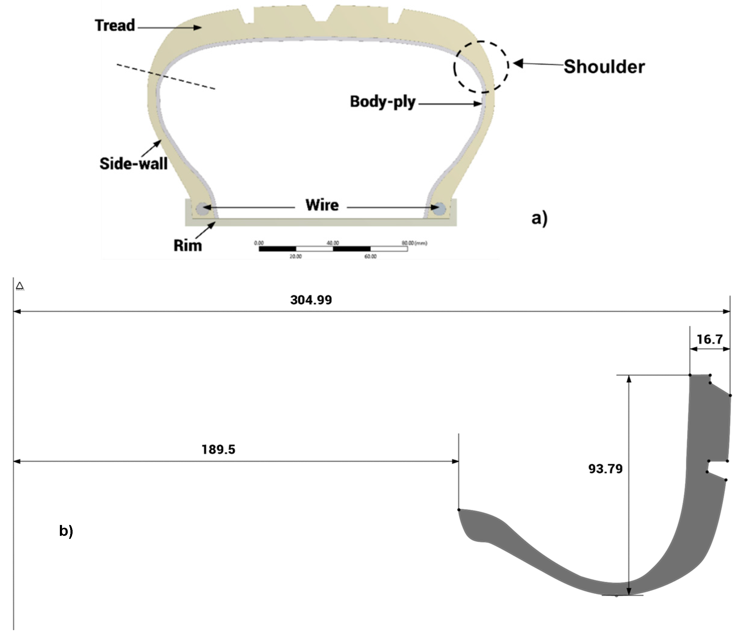
- It was supposed that the tire was made of steel bead wires, rubber, cord plies, and rim.
- The rubber was considered homogenous, isotropic, and hyperelastic over the whole temperature range.
- It was assumed that the steel bead wire, rim, and cord ply were homogenous, isotropic, and elastic materials.
- It was assumed that the road and the rim were rigid.
- It was assumed that the friction coefficient between the road and the tire was constant at 0.1, while neglecting the fluctuation in the amount of friction between the road and tire. Then, the friction coefficient was changed to investigate the effect of this variable on the distribution of temperature within the rubber.
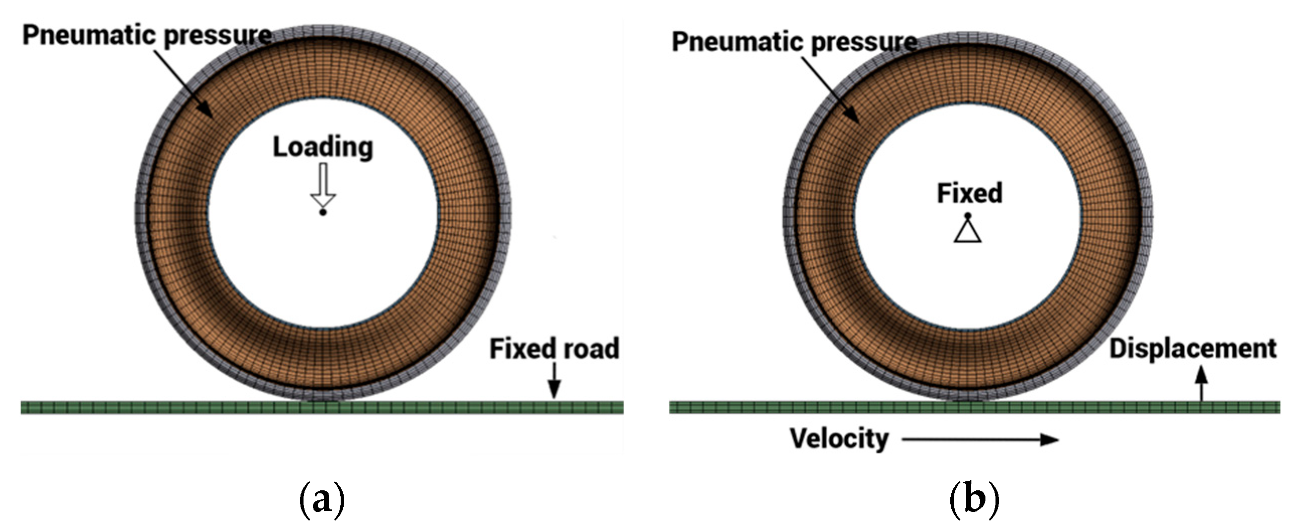
2.1. Dynamic Rolling Analysis
- Step 1:
- Loading Analysis
- Step 2:
- Rolling Analysis
2.2. Steady-State Thermal Analysis
3. Conceptual Modeling of Rubber Materials
3.1. Model for Hyperelastic Material by Mooney–Rivlin Function
3.2. Heat Generation Rate
4. Simulation and Thermo-Investigation of Rolling Tires on the Flat Road Affected by Some Factors
4.1. Mesh Sensitivity Study
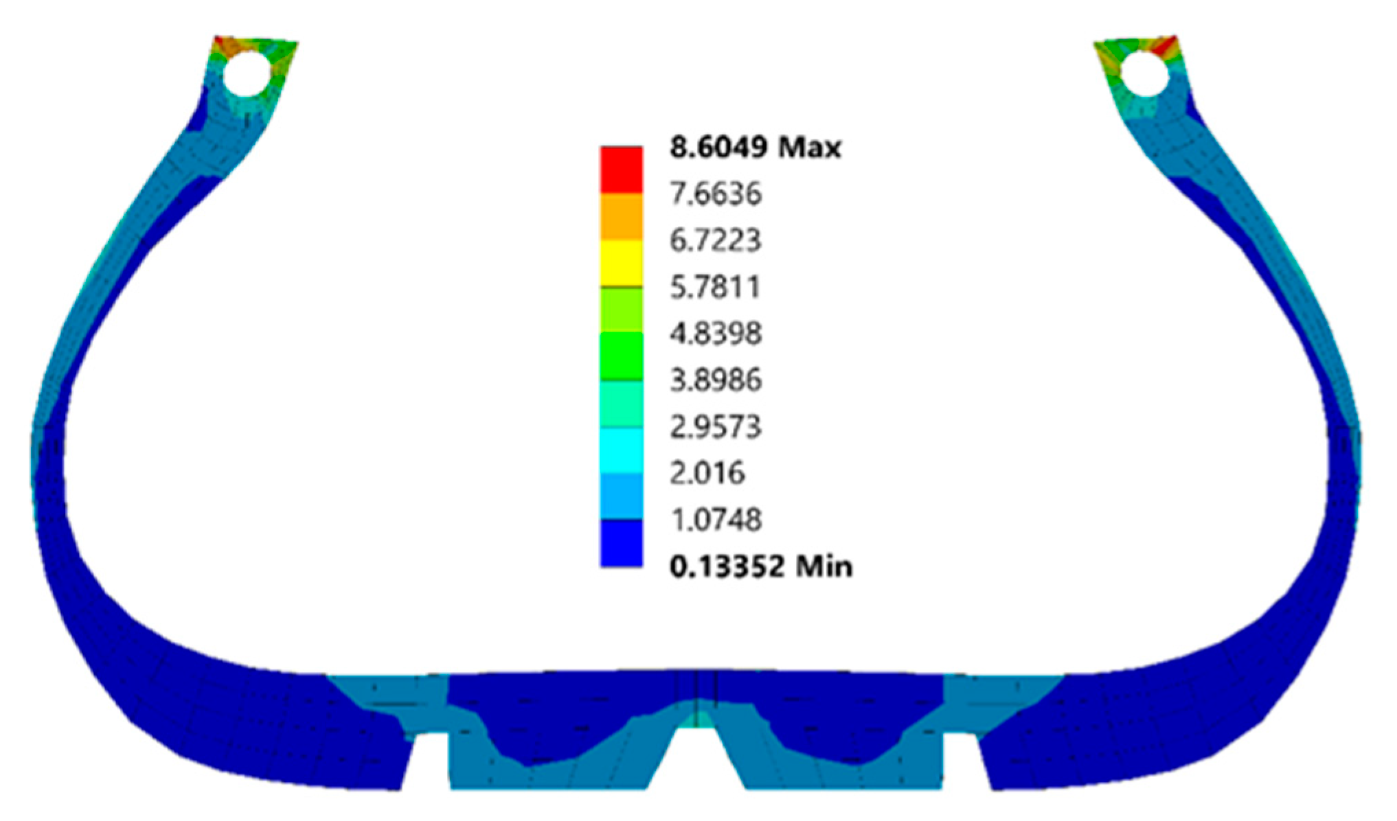
4.2. Loading and Rolling Analysis
4.3. Thermal Analysis
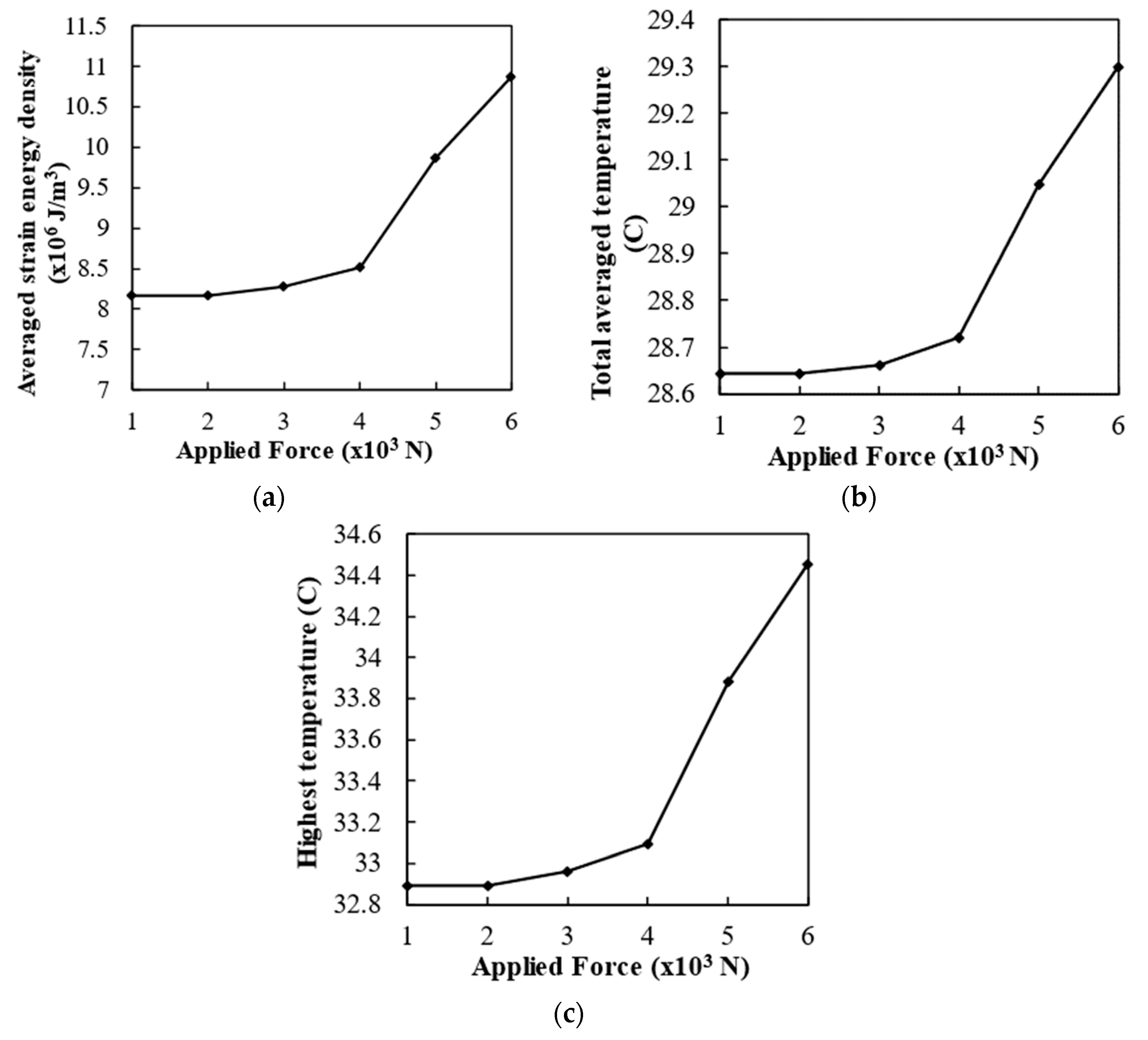
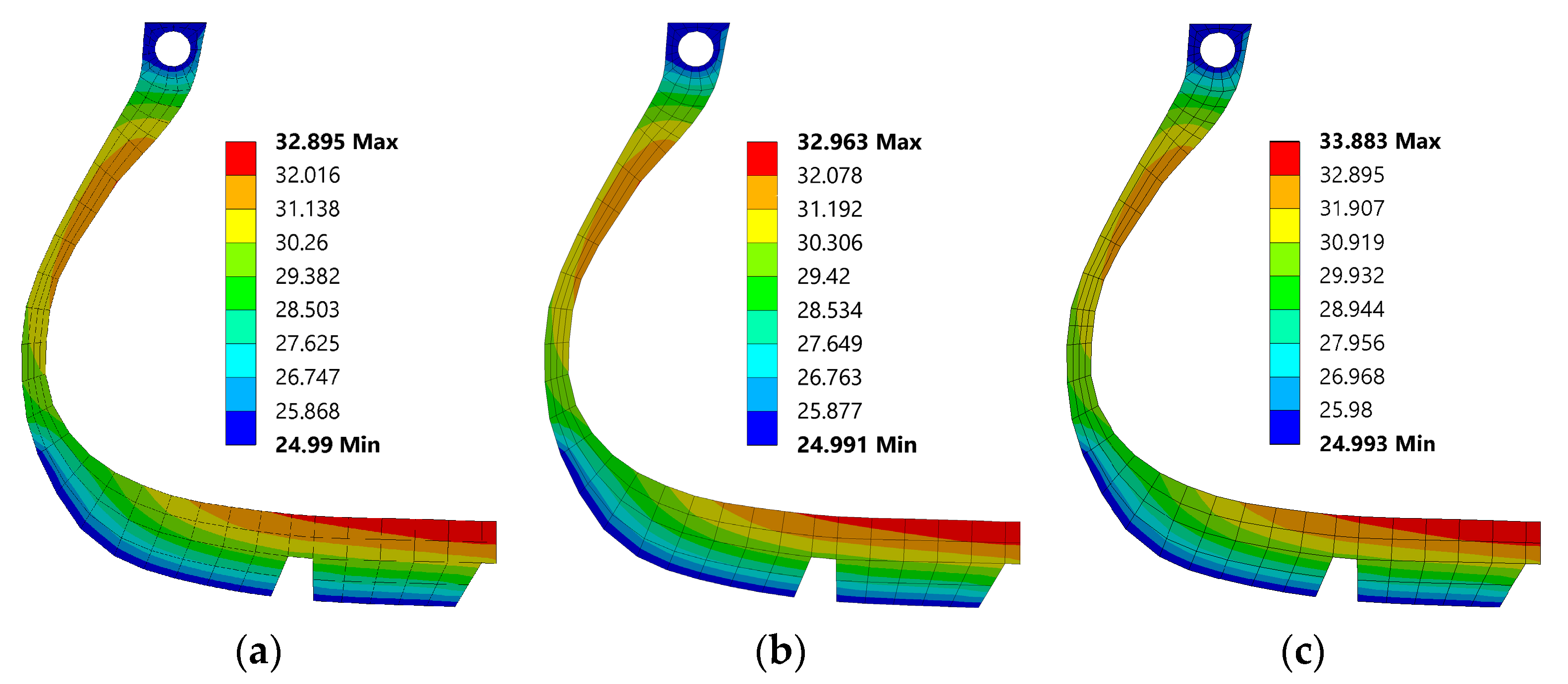
4.3.1. Change in Loading
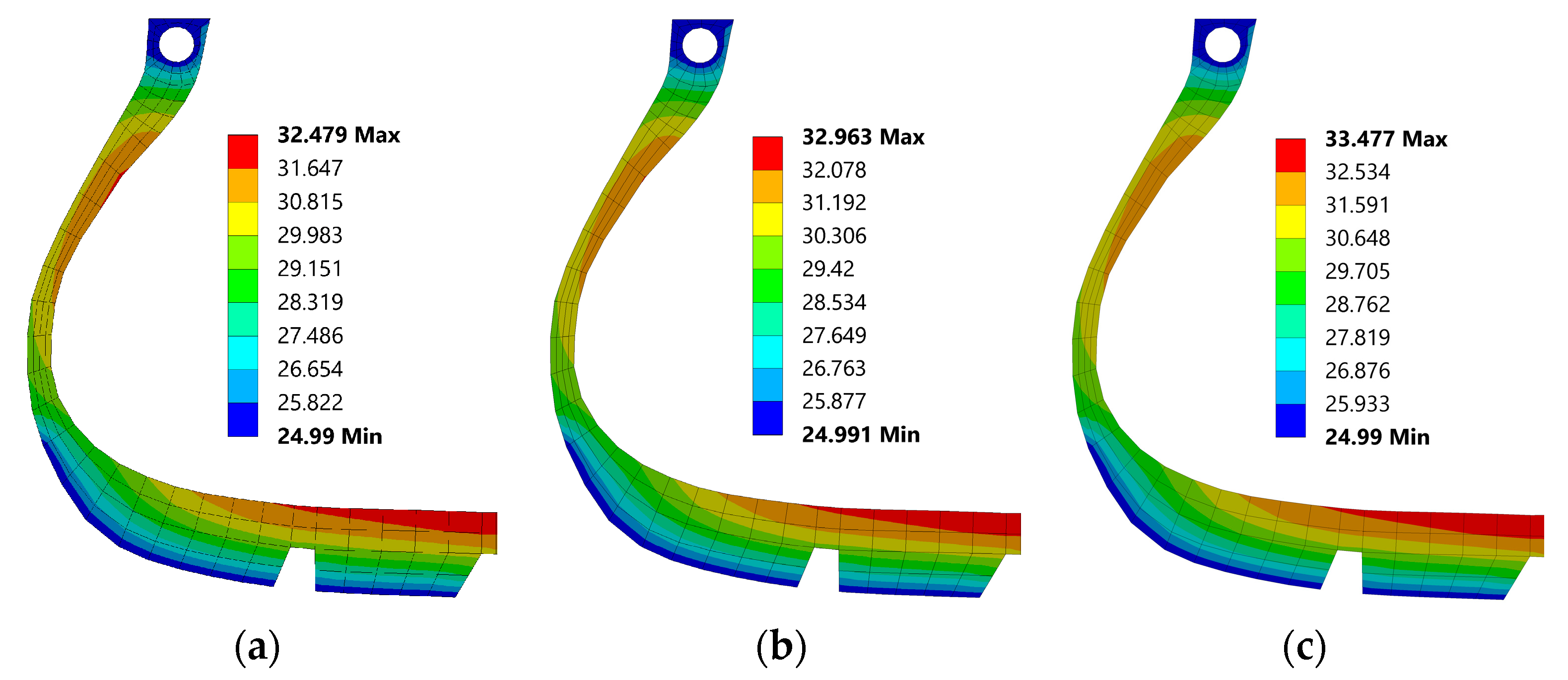
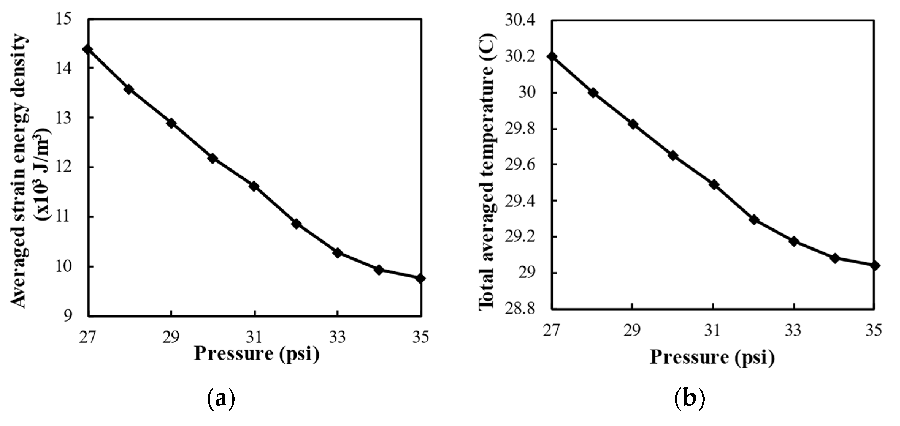
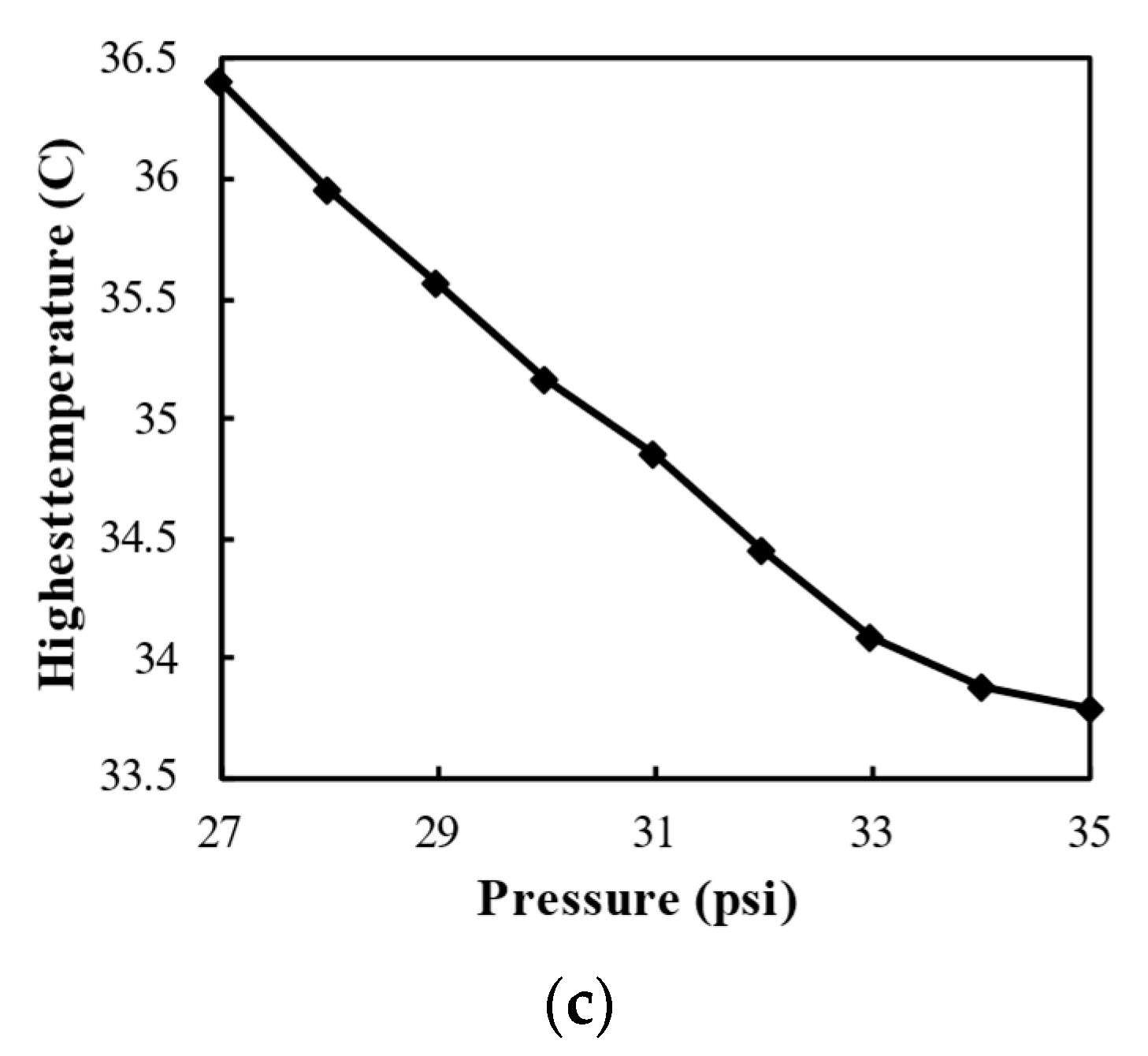
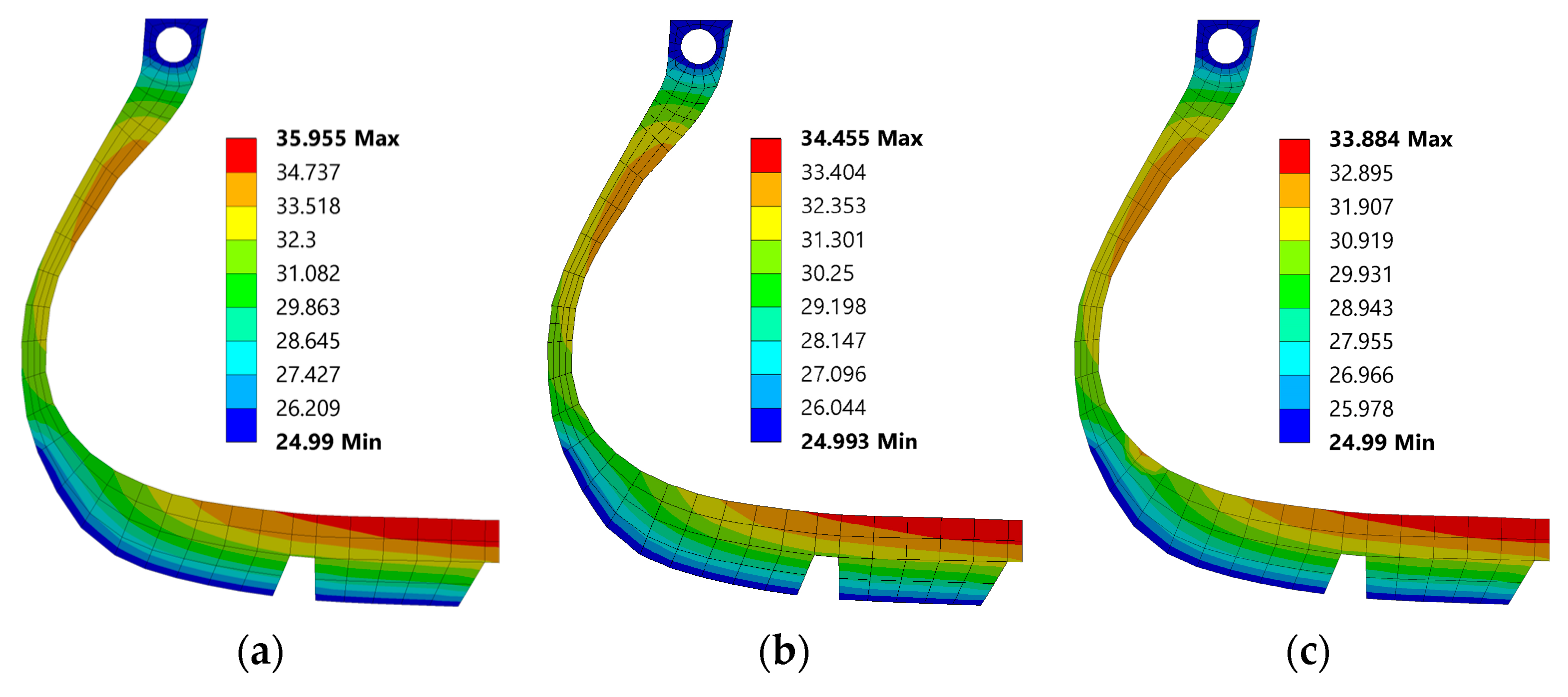
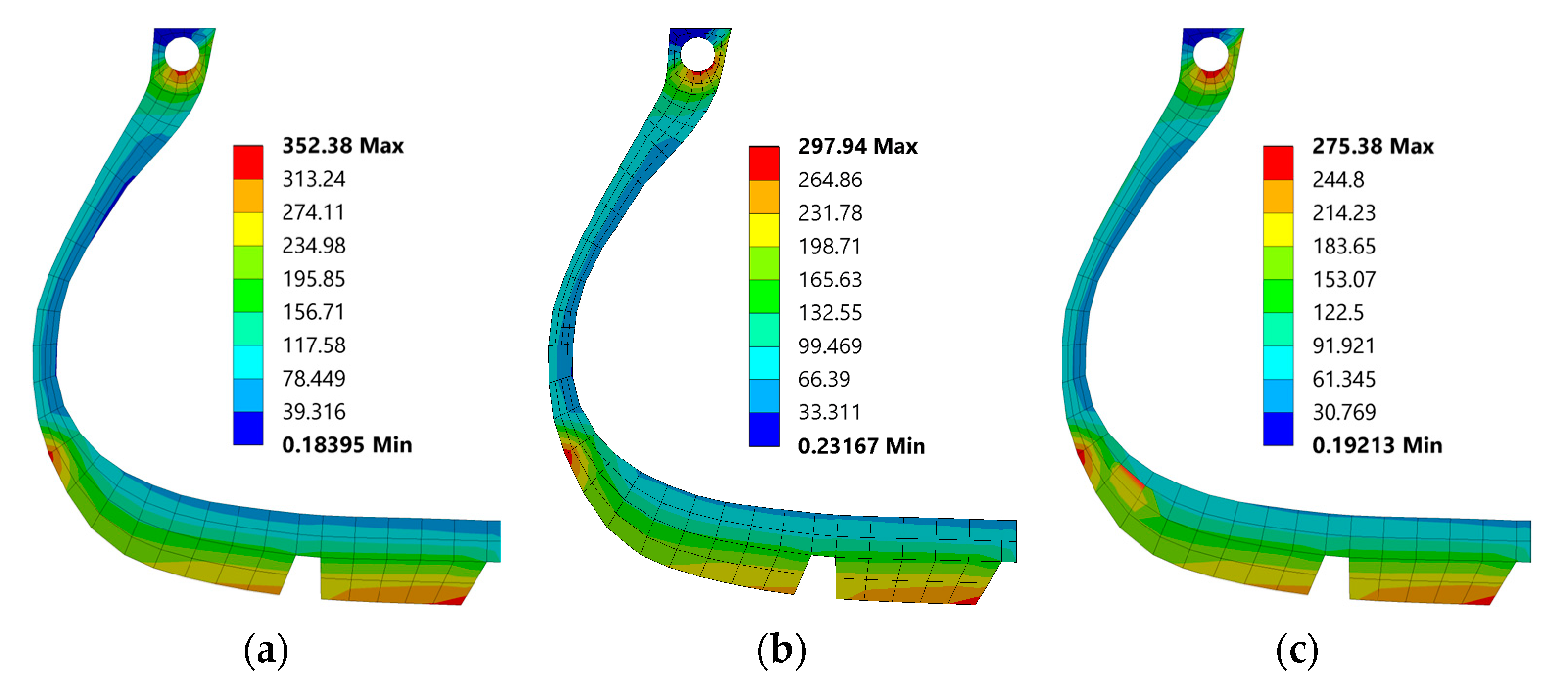
4.3.2. Change in Pressure
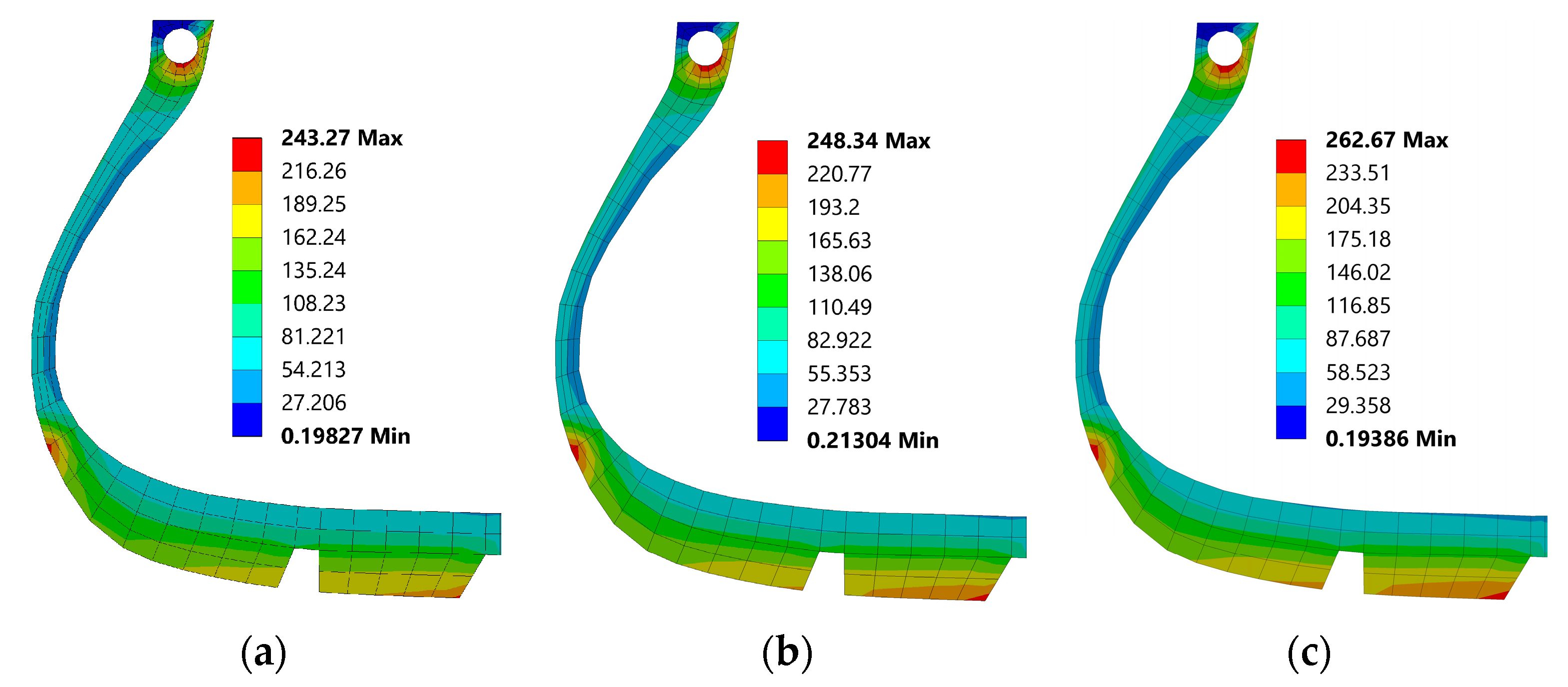
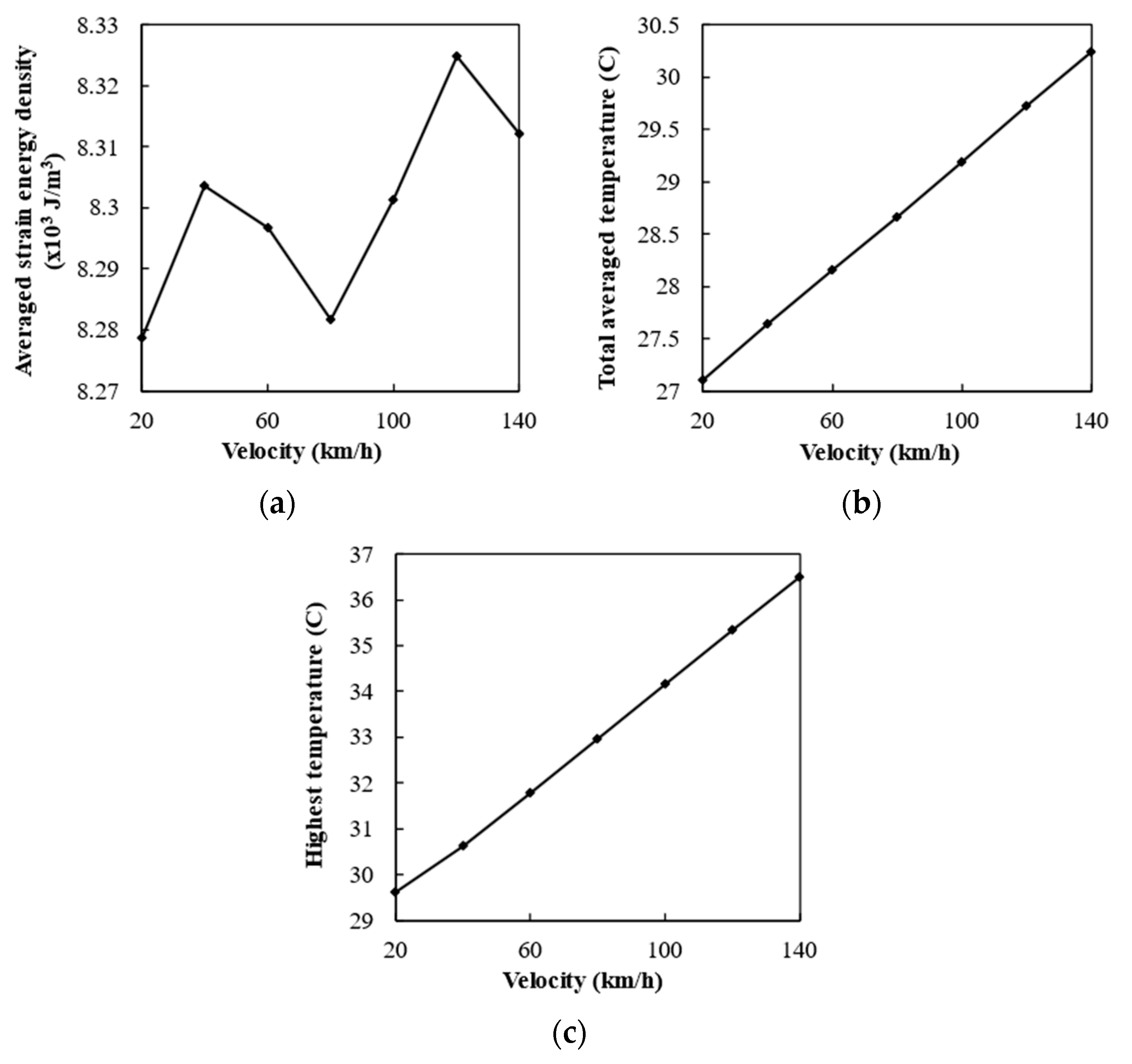
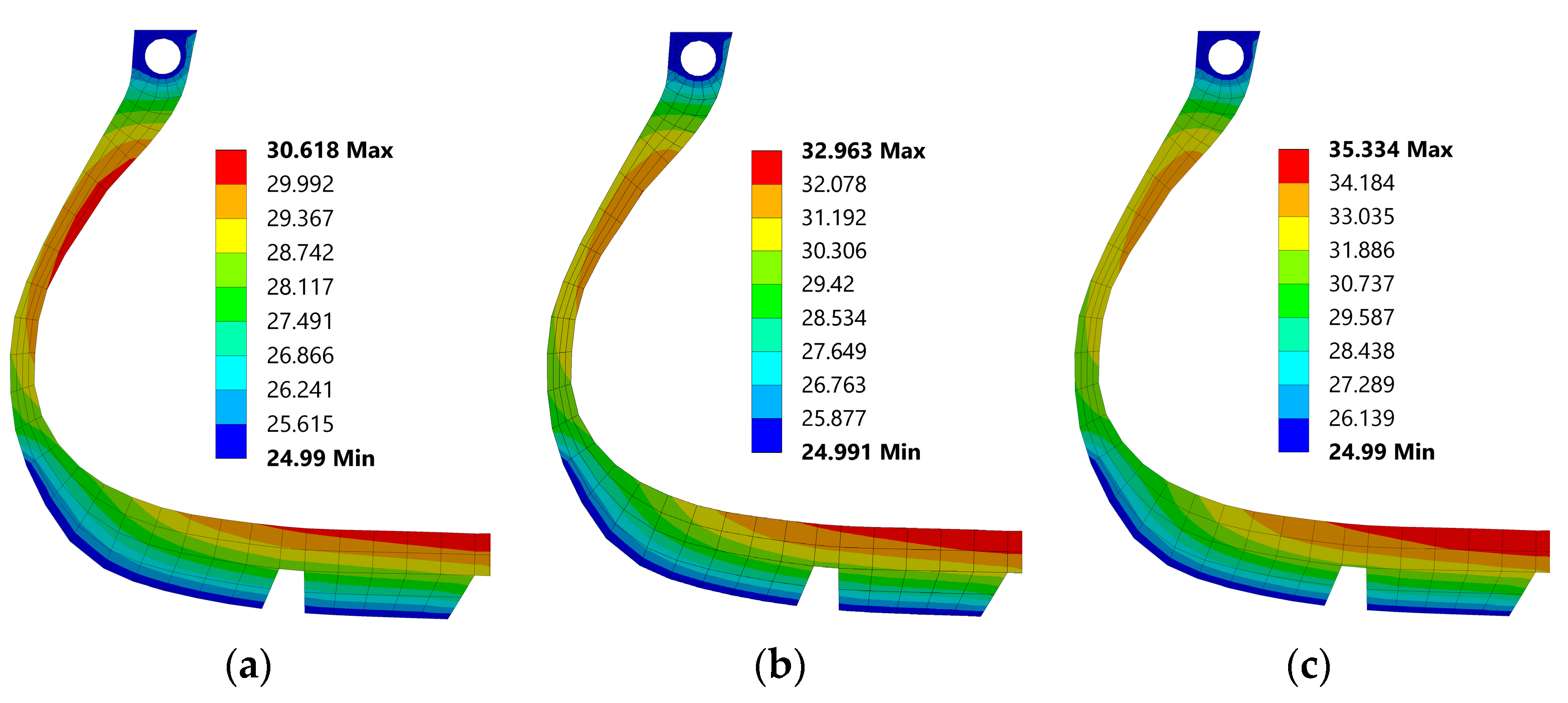
4.3.3. Change in Velocity
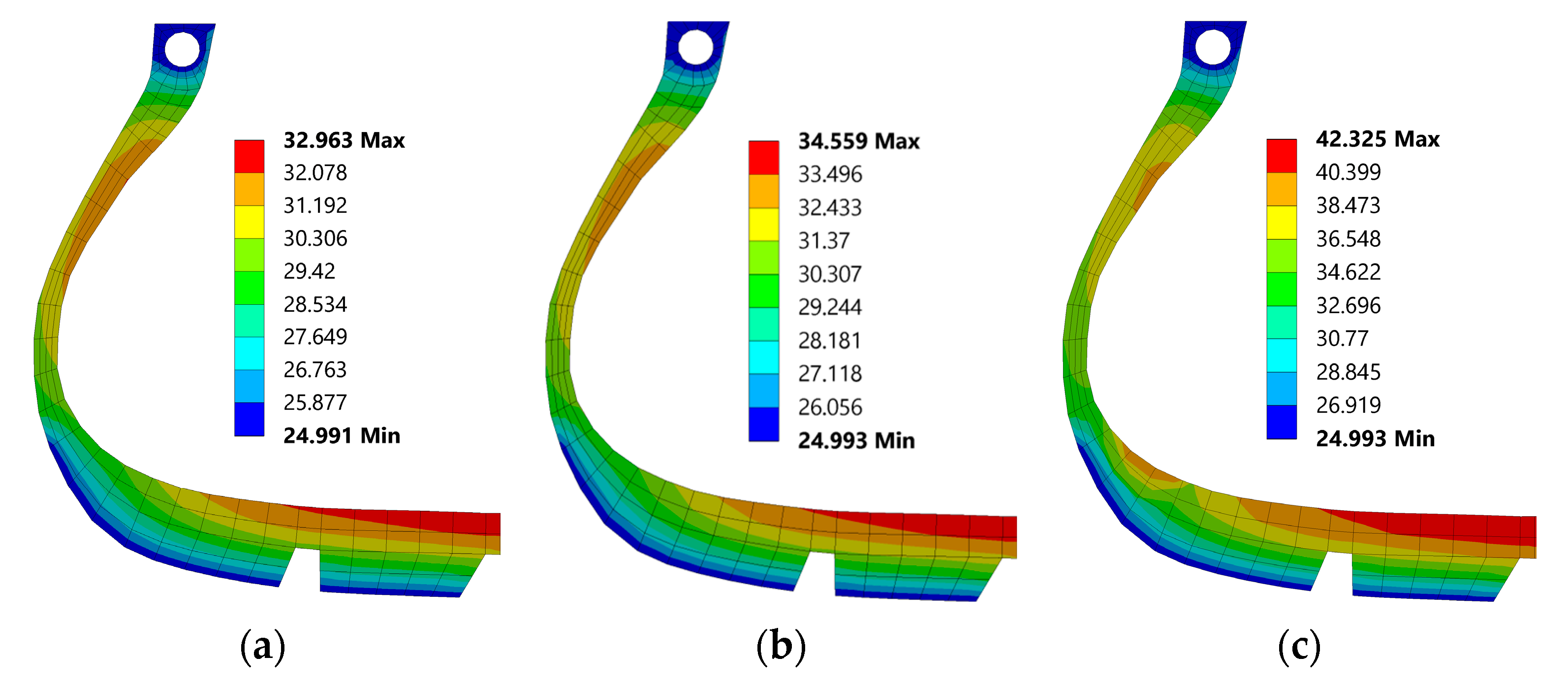
4.3.4. Change in Friction Coefficient between the Road and the Rubber
5. Conclusions
Author Contributions
Funding
Institutional Review Board Statement
Informed Consent Statement
Data Availability Statement
Acknowledgments
Conflicts of Interest
References
- Kainradl, P.; Kaufmann, G. Heat generation in pneumatic tires. Rubber Chem. Technol. 1976, 49, 823–861. [Google Scholar] [CrossRef]
- Conant, F.S. Tire Temperatures. Rubber Chem. Technol. 1971, 44, 397–439. [Google Scholar] [CrossRef]
- Schuring, D.J.; Futamura, S. Rolling loss of pneumatic highway tires in the eighties. Rubber Chem. Technol. 1990, 63, 315–367. [Google Scholar] [CrossRef]
- Fervers, C.W. Improved FEM simulation model for tire–soil interaction. J. Terramechanics 2004, 41, 87–100. [Google Scholar] [CrossRef]
- Hölscher, H.; Tewes, M.; Botkin, N.; Loehndorf, M.; Hoffmann, K.; Quandt, E. Modeling of Pneumatic Tires by a Finite Element Model for the Development a Tire Friction Remote Sensor. J. S. Afr. Inst. Mech. Eng. 2004, 35, 21–30. [Google Scholar]
- Reida, J.D.; Boesch, D.A.; Bielenberg, R.W. Detailed tire modeling for crash applications. Int. J. Crashworthiness 2007, 12, 521–529. [Google Scholar] [CrossRef]
- Yanjin, G.; Guoqun, Z.; Gang, C. Influence of belt cord angle on radial tire under different rolling states. J. Reinf. Plast. Compos. 2006, 25, 1059–1077. [Google Scholar] [CrossRef]
- Clark, S.K. Mechanics of Pneumatic Tires; US Government Printing Office: Washington, DC, USA, 1981.
- Sokolov, S.L. Analysis of the heat state of pneumatic tires by the finite element method. J. Mach. Manuf. Reliab. 2009, 38, 310–314. [Google Scholar] [CrossRef]
- Ebbott, T.G.; Hohman, R.L.; Jeusette, J.P.; Kerchman, V. Tire Temperature and Rolling Resistance Prediction with Finite Element Analysis. Tire Sci. Technol. 1999, 27, 2–21. [Google Scholar] [CrossRef]
- Nallusamy, S.; Rajaram Narayanan, M.; Suganthini Rekha, R. Design and performance analysis of vehicle tyre pattern material using finite element analysis and ANSYS R16.2. Key Eng. Mater. 2018, 777, 426–431. [Google Scholar] [CrossRef]
- Kar, K.K.; Bhowmick, A.K. Hysteresis loss in filled rubber vulcanizates and its relationship with heat generation. J. Appl. Polym. Sci. 1997, 64, 1541–1555. [Google Scholar] [CrossRef]
- Park, D.M.; Hong, W.H.; Kim, S.G.; Kim, H.J. Heat generation of filled rubber vulcanizates and its relationship with vulcanizate network structures. Eur. Polym. J. 2000, 36, 2429–2436. [Google Scholar] [CrossRef]
- Park, H.C.; Youn, S.K.; Song, T.S.; Kini, N.J. Analysis of Temperature Distribution in a Rolling Tire Due to Strain Energy Dissipation. Tire Sci. Technol. 1997, 25, 214–228. [Google Scholar] [CrossRef]
- Giurgiu, T.; Ciortan, F.; Pupaza, C. Static and Transient Analysis of Radial Tires Using ANSYS. Recent Advances in Industrial and Manufacturing Technologies. In Proceedings of the 1st International Conference on Industrial and Manufacturing Technologies (INMAT’13), Vouliagmeni, Athens, Greece, 14–16 May 2013; pp. 148–152. [Google Scholar]
- De Gregoriis, D.; Naets, F.; Kindt, P.; Desmet, W. Development and validation of a fully predictive high-fidelity simulation approach for predicting coarse road dynamic tire/road rolling contact forces. J. Sound Vib. 2019, 452, 147–168. [Google Scholar] [CrossRef]
- Johnson, A.R.; Chen, T. Coupled Thermo-Mechanical Analyses of Dynamically Loaded Rubber Cylinders. In Proceedings of the 2nd International SAMPE Technical Conference, Boston, MA, USA, 25–30 June 2001; Volume 32, pp. 360–371. [Google Scholar]
- Kan, Q.; Kang, G.; Yan, W.; Zhu, Y.; Jiang, H. A thermo-mechanically coupled cyclic plasticity model at large deformations considering inelastic heat generation. In Proceedings of the 13th International Conference on Fracture (ICF 2013), Beijing, China, 16–21 June 2013; Volume 5, pp. 854–3863. [Google Scholar]
- Martin, J.W.; Martin, T.J.; Bennett, T.P.; Martin, K.M. Surface Mining Equipment, 1st ed.; Martin Consultants, Inc.: Golden, CO, USA, 1982. [Google Scholar]
- Caterpillar. Caterpillar Performance Handbook, 46th ed.; Caterpillar Inc.: Peoria, IL, USA, 2016. [Google Scholar]
- Schuring, D.J. Rolling loss of pneumatic tires. Rubber Chem. Technol. 1980, 53, 600–727. [Google Scholar] [CrossRef]
- Tang, T.; Johnson, D.; Smith, R.E.; Felicelli, S.D. Numerical evaluation of the temperature field of steady-state rolling tires. Appl. Math. Model. 2014, 38, 1622–1637. [Google Scholar] [CrossRef]
- Zang, L.; Cai, Y.; Wang, B.; Yin, R.; Lin, F.; Hang, P. Optimization design of heat dissipation structure of inserts supporting run-flat tire. Proc. Inst. Mech. Eng. Part D J. Automob. Eng. 2019, 233, 3746–3757. [Google Scholar] [CrossRef]
- Hall, D.E.; Moreland, J.C. Fundamentals of Rolling Resistance. Rubber Chem. Technol. 2001, 74, 525–539. [Google Scholar] [CrossRef]
- De Beer, M.; Maina, J.W.; van Rensburg, Y.; Greben, J.M. Toward Using Tire-Road Contact Stresses in Pavement Design and Analysis. Tire Sci. Technol. 2012, 40, 246–271. [Google Scholar] [CrossRef]
- Wang, H.; Al-Qadi, I.L.; Stanciulescu, I. Simulation of tyre–pavement interaction for predicting contact stresses at static and various rolling conditions. Int. J. Pavement Eng. 2011, 13, 310–321. [Google Scholar] [CrossRef]
- Douglas, R.A.; Alabaster, D.; Charters, N. Measured tire/road contact stresses characterized by tire type, wheel load, and inflation pressure. In TAC/ATC 2008—2008 Annual Conference and Exhibition of the Transportation Association of Canada: Transportation—A Key to a Sustainable Future; Transportation Association of Canada (TAC): Ottawa, ON, Canada, 2008. [Google Scholar]
- ANSYS Workbench 19.1; ANSYS Inc.: Canonsburg, PA, USA, 2018.
- Lin, Y.J.; Hwang, S.J. Temperature prediction of rolling tires by computer simulation. Math. Comput. Simul. 2004, 67, 235–249. [Google Scholar] [CrossRef]
- Smith, R.E.; Tang, T.; Johnson, D.; Ledbury, E.; Goddette, T.; Felicelli, S.D. Simulation of Thermal Signature of Tires and Tracks; Mississippi State Univ Mississippi State Center for Advanced Vehicular Systems: Starkville, MS, USA, 2012. [Google Scholar]


| Material | Rubber | Body-Ply | Bead Wire |
|---|---|---|---|
| Density (kg/m3) | 1400 | 1200 | 6500 |
| Poisson’s ratio | - | 0.3 | 0.3 |
| Young’s modulus (Mpa) | - | 500 | 207 |
| Mooney–Rivlin constant (Mpa) | C10 = 8.061 | - | - |
| C01 = 1.805 | - | - | |
| Thermal conductivity (W/m·°C) | 0.293 | 0.293 | 60.5 |
| Hysteresis | 0.1 | - | - |
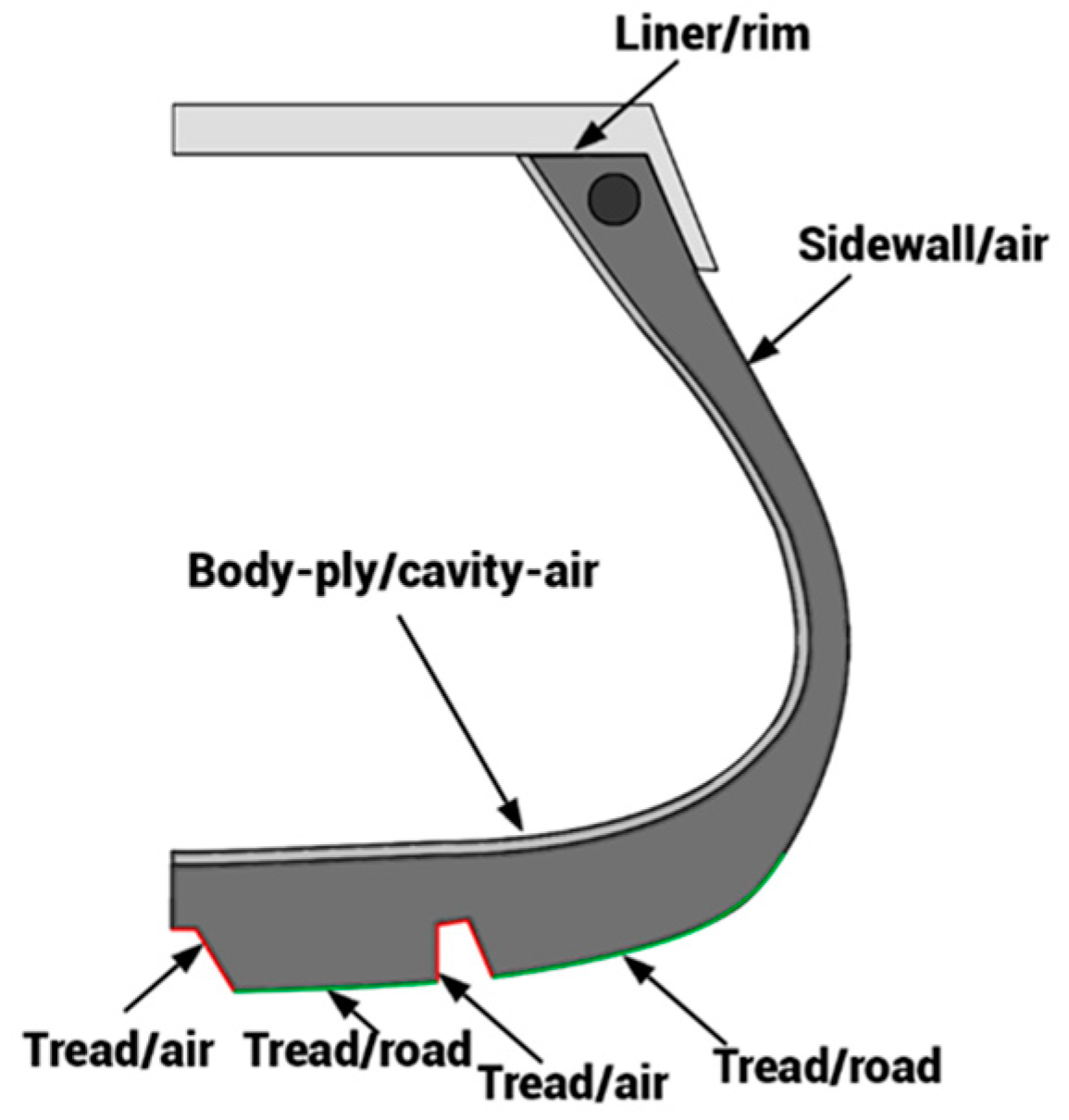
| Location | Heat Transfer Coefficient (W/m2·K) | Sink Temperature (°C) |
|---|---|---|
| Tread/road | 12,000 | 25 |
| Tread/air | 16.18 | 25 |
| Sidewall/air | 16.18 | 25 |
| Body-ply/cavity-air | 5.9 | 38 |
| Liner/rim | 88,000 | 25 |
| Mesh No. | No. Perimeter Divisions | Rubber | Body-Ply | Rim | Bead Wire | Total Elements | Tire Displacement (mm) |
|---|---|---|---|---|---|---|---|
| 1 | 92 | 18,321 | 3412 | 2893 | 1423 | 27,471 | 5.82 |
| 2 | 104 | 23,657 | 4562 | 3718 | 1885 | 35,705 | 6.96 |
| 3 | 120 | 30,624 | 5800 | 4872 | 2320 | 45,936 | 7.70 |
| 4 | 140 | 39,711 | 7740 | 6434 | 3056 | 59,997 | 7.78 |
| 5 | 160 | 51,955 | 9902 | 8334 | 3921 | 78,032 | 7.81 |
| Parameters | Ref. Value | Min | Max | Step |
|---|---|---|---|---|
| Weight (N) | 3000 | 1000 | 6000 | 1000 |
| Pressure (psi) | 32 | 27 | 35 | 1 |
| Velocity (km/h) | 80 | 20 | 140 | 20 |
Disclaimer/Publisher’s Note: The statements, opinions and data contained in all publications are solely those of the individual author(s) and contributor(s) and not of MDPI and/or the editor(s). MDPI and/or the editor(s) disclaim responsibility for any injury to people or property resulting from any ideas, methods, instructions or products referred to in the content. |
© 2023 by the authors. Licensee MDPI, Basel, Switzerland. This article is an open access article distributed under the terms and conditions of the Creative Commons Attribution (CC BY) license (https://creativecommons.org/licenses/by/4.0/).
Share and Cite
Nguyen, T.-C.; Cong, K.-D.D.; Dinh, C.-T. Rolling Tires on the Flat Road: Thermo-Investigation with Changing Conditions through Numerical Simulation. Appl. Sci. 2023, 13, 4834. https://doi.org/10.3390/app13084834
Nguyen T-C, Cong K-DD, Dinh C-T. Rolling Tires on the Flat Road: Thermo-Investigation with Changing Conditions through Numerical Simulation. Applied Sciences. 2023; 13(8):4834. https://doi.org/10.3390/app13084834
Chicago/Turabian StyleNguyen, Thanh-Cong, Khanh-Duy Do Cong, and Cong-Truong Dinh. 2023. "Rolling Tires on the Flat Road: Thermo-Investigation with Changing Conditions through Numerical Simulation" Applied Sciences 13, no. 8: 4834. https://doi.org/10.3390/app13084834
APA StyleNguyen, T.-C., Cong, K.-D. D., & Dinh, C.-T. (2023). Rolling Tires on the Flat Road: Thermo-Investigation with Changing Conditions through Numerical Simulation. Applied Sciences, 13(8), 4834. https://doi.org/10.3390/app13084834