Two-Dimensional Space Turntable Pitch Axis Trajectory Prediction Method Based on Sun Vector and CNN-LSTM Model

Abstract

A two-dimensional space turntable system has been used to ensure that the Solar X-ray and Extreme Ultraviolet Imager (X-EUVI) can track the Sun stably, and the prediction of the two-dimensional turntable trajectory is an important part of payload health management. Different from the dynamic model using traditional trajectory prediction, we propose a new method for predicting the pitch axis trajectory of the turntable based on the sun vector and a deep learning CNN-LSTM model. First, the ideal solar position of the pitch axis was calculated using the sun vector. Then, the ideal solar position was combined with the running turntable pitch axis motor speed, current, and solar position error signal as the CNN-LSTM model input data. The model parameters were trained and adjusted through test data simulation using Fengyun-3E satellite orbit data. Finally, the next position of the pitch axis was predicted. The test results showed that in the sun vector and CNN-LSTM model, the RMSE value was 0.623 and the MSE value was 0.388. It was better than the LSTM model or CNN model alone and could accurately predict the pitch axis position.

1. Introduction

The Solar X-ray and Extreme Ultraviolet Imager (X-EUVI) is a payload of the Sun synchronous orbit (twilight) FY-3E satellite, which has an orbital altitude of 836 km and an orbital period of 102 min. This is the first space-based solar X-ray and extreme ultraviolet (EUV) imager for space weather and space physics in China [1]. FY-3E is a three-axis stabilized spacecraft with respect to the Earth and changes in the position of the Sun the X-EUVI coordinate system in real time. Therefore, the two-dimensional turntable system was developed to track the Sun [1]. It is shown in Figure 1.

When X-EUVI works in orbit, the two-dimensional turntable system first roughly points to the Sun according to the sun vector from the satellite. Then, X-EUVI precisely points to the Sun using a turntable lock-in control system based on Trace Guide Telescope (TGT) solar position data [1].

The two-dimensional turntable includes the pitch axis and the azimuth axis. The control system of the two-dimensional turntable realizes the accurate direction of the target by controlling the position, speed, and torque of the two brushless motors, namely the position axis and the pitch axis [2]. This paper takes the pitch axis trajectory as the research object. The two-dimensional turntable controls the trajectory depending on the sun vector data and the solar position data combined with the satellite attitude and other factors.

When the turntable controls the optical axis to point to the sun, the image obtained by the XEUV is in the center of the field of view as shown in Figure 2.

The main factors affecting the normal running of the turntable include the turntable motor current, motor voltage, target solar position, and solar position error signal. The prediction of the two-dimensional turntable trajectory can show the operation status of the turntable. It is not only important to understand the operation of the turntable itself but also that it has an important impact on the evaluation of the operation status of the satellite platform. The same applies to the trajectory prediction of the spaceborne integrated platform or intelligent load.

The existing models of trajectory prediction involve different algorithms in different fields, but research on trajectory predictions of a two-dimensional turntable in space is still lacking. By establishing the traditional motion model, the running track of the turntable can be predicted. However, due to many unknown and variable factors in the model, the error is difficult to measure, so the accuracy of the motion model is difficult to guarantee [3]. There are many different methods for trajectory prediction. They include the hidden Markov model (HMM), based on mathematical statistical methods [4], the Kalman filter [5], or neural networks and deep learning in machine learning methods [6,7,8,9,10]. The advantage of the hidden Markov model is that it has a relatively good prediction effect for tracks with variable states, and the disadvantage is that because of its memoryless nature, it cannot use the preorder information of track sequence. The hidden Markov model is often used for long-sequence prediction [11]. It is often used for pedestrian trajectory prediction. A Kalman filter relies on the information of the previous sequence point and the current position information to predict the next moment. The advantage is that the state estimation process is very stable, and because its calculation process is a continuous prediction and correction process, it is suitable for trajectory-prediction scenarios requiring strong real-time performance. However, the Kalman filter is extremely dependent on forecasting the next time based on the information of the last sequence point and the current position information.

Neural networks and deep learning have strong nonlinear mapping, self-learning, and adaptive abilities. The disadvantage is that they are very sensitive to the initial network’s weight, and there is a local minimization problem. When the initial network weight is not uniform, the training results may be different, so this method is applicable to most trajectory prediction scenarios. Since there is no uniform standard for the structure of a neural network, the appropriate network structure should be selected according to the specific situation in practical application [12].

We proposed to use a sun vector and a one-dimensional convolutional neural network combined with a long short-term memory network (CNN-LSTM) hybrid neural network model as a method for predicting the trajectory of the pitch axis of the space turntable. First, according to the sun position calculation model, we calculated the ideal solar position value from the sun vector data and then used the ideal solar position value of the pitch axis, pitch axis motor speed, current, and position error signal data as the input data of the model. We then selected a specific step of the time sliding window and predicted the position of the pitch axis at the next time. It was built on a model of CNN-LSTM, the prediction sequence was set with an adaptive Adam optimizer, and the simulating telemetry data of a two-dimensional turntable was used for training. We used RMSE and MSE as performance evaluation indicators.

2. Materials and Methods

The pitch axis pointing model established a two-dimensional turntable to roughly point to the Sun from the sun vector broadcasted by the satellite platform.

2.1. Sun Vector Calculat Model

The sun vector in the orbital instant root broadcast was the unit vector in the orbital coordinate system. The sun vector was defined using the J2000 coordinate system [13,14]. After a series of coordinate transformations from the orbit coordinate system to the unit vector of the optical axis of the guide mirror, the transformation matrix of the satellite attitude had to be considered as shown in Figure 1. Many error factors were difficult to determine, setting all the installation errors was ignored, and the satellite attitude was ignored so the ideal value of the turntable motion could be calculated.

The ideal position value of the pitch axis can be calculated through the sun vector. It is shown in Equations (1) and (2):

Sun vector:

$$S_0={\left[Xs\left(t\right)Ys\left(t\right)Zs\left(t\right)\right]}^T$$

(1)

We calculated the ideal value of the pitch axis of the turntable as:

$${\theta }_{pitcht}=\mathrm{atan}\left[\frac{Zs\left(t\right)}{Ys\left(t\right)}\right]\times D_{pitcht}$$

(2)

where S₀ is the sun vector, ${\theta }_{pitcht}$ is the pitch axis angle, and $D_{pitcht}$ is the error matrix, which is currently set as the unit matrix. According to the above formula, the initial position of the pitch angle of the turntable could be calculated in advance through the sun vector data broadcasted by the satellite platform. In the actual operation of the turntable, the platform attitude factor and the position error should also be considered. In addition, it was also affected by the operating speed and control current of the turntable itself.

2.2. One-Dimensional Convolution Neural Network (1D-CNN) Model

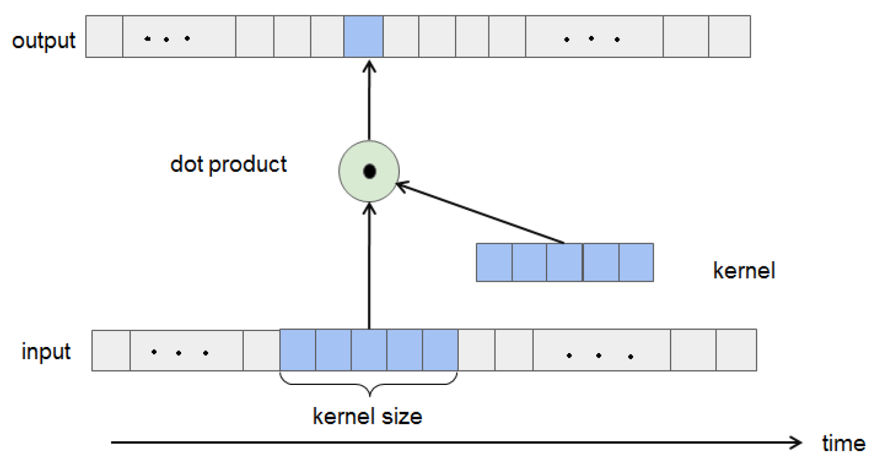
CNN is a successful deep learning framework first proposed by LeCun et al. [15]. In the study of deep learning, in 1D-CNN (also known as time-domain convolution), the convolution kernel is a vector with a length of N, which is used for neighborhood filtering of one-dimensional input signals and extracting local features. The kernel slides along a one-dimensional time axis. It is often used to process NLP and time series data. It is shown in Figure 3.

In the convolution layer, the input data information needs to undergo convolution operation and activation function calculation before flowing to the next layer. The operation is shown in Equation (3):

$$h_t={\sigma }_{cnn}\left(W_{cnn}\ast X_t+b_{cnn}\right)$$

(3)

where $W_{cnn}$ represents the weight coefficient of the filter, namely the convolution kernel; $X_t$ represents the data information of the time, while the input sample * represents the discrete convolution operation between $X_t$ and $W_{cnn}$; $b_{cnn}$ is a bias parameter, which will be obtained by learning when training the model; σ Cnn stands for the activation function; and $h_t$ represents the output data after the convolution operation.

2.3. Long Short-Term Memory (LSTM) Network Model

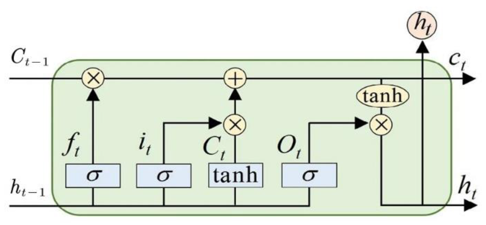
A long short-term memory network (LSTM) is an improved cyclic neural network used to solve the problem that RNN networks cannot deal with long-distance dependence. Hochreiter proposed the LSTM algorithm [16], which can store data information in a longer time step. Regarding the problem of time series prediction and analysis, LSTM can predict future data characteristics through the data characteristics of the past period time. LSTM networks enable nodes to “remember” or “forget” data through a “gate” structure, which mainly includes three “gates”: the forgetting gate, the information adding a gate, and the information output gate. Through these three “gates”, the input of each cell state contains the output of the previous moment, and the input of the current moment also contains some information stored by the node itself. Therefore, LSTM has a better performance on longer sequences. It is shown in Figure 4.

The LSTM updates for time steps given inputs x_t, h_t−1, and C_t−1, The operation is shown in Equations (4)–(9):

$$f_t=\sigma \left(W_f\cdot \left[C_{t-1},h_{t-1},x_t\right]+b_f\right)$$

(4)

$$i_t=\sigma \left(W_i\cdot \left[C_{t-1},h_{t-1},x_t\right]+b_i\right)$$

(5)

$${\tilde{C}}_t=\tanh \left(W_C\cdot \left[h_{t-1},x_t\right]+b_C\right)$$

(6)

$$C_t=f_t\ast C_{t-1}+i_t\ast {\tilde{C}}_t$$

(7)

$$o_t=\sigma \left(W_o\left[h_{t-1},x_t\right]+b_o\right)$$

(8)

$$h_t=o_t\ast \tanh \left(C_t\right)$$

(9)

where σ and tanh represent the sigmoid activation function and hyperbolic tangent activation function, respectively; W and b represent the weight matrix and bias parameters, respectively; x_t represents the input of the LSTM unit at time t; h_t represents the output of the unit corresponding to at time t; and C_t represents the state unit of the LSTM at time t. The whole LSTM unit includes three thresholds, namely forgetting gate f_t, input gate i_t, and output gate o_t.

2.4. CNN-LSTM Model

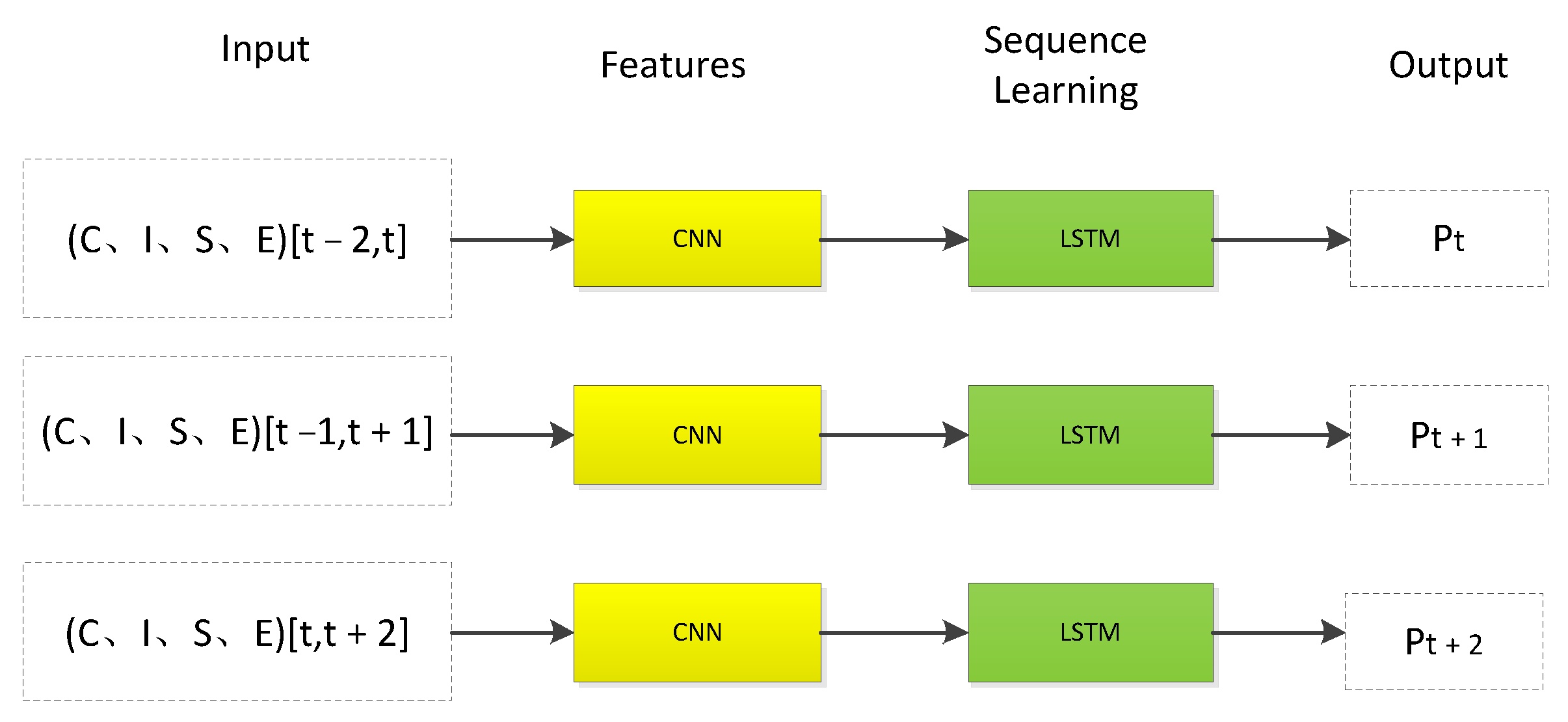
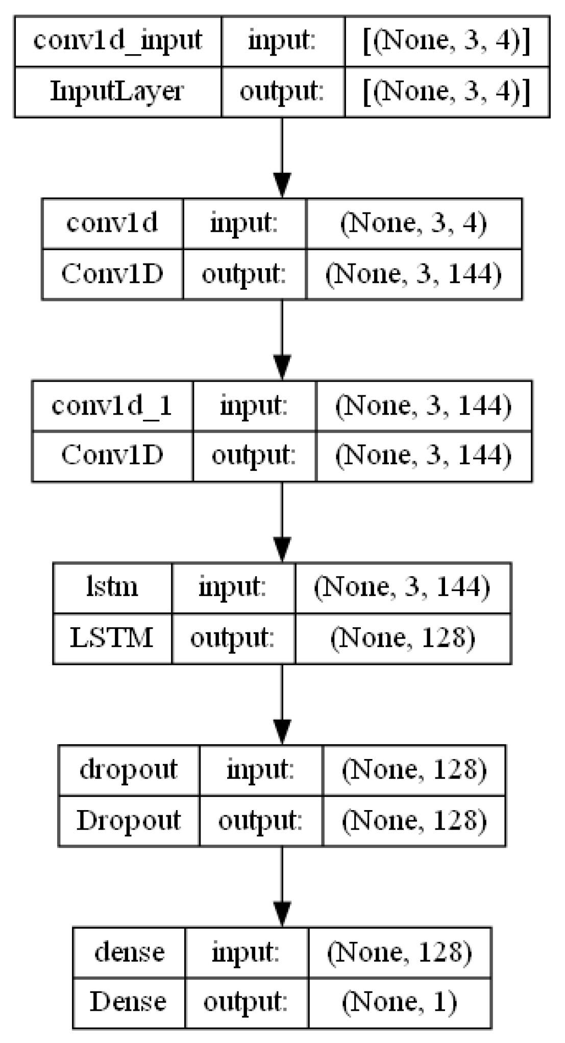
The CNN-LSTM model is a hybrid model of two neural network models. We first used CNN to extract data features and LSTM to further extract temporal features. The specific structure was as follows: the CNN model used a Conv1D layer and multiple input data as the time series; the kernel moved in one dimension along the time axis, then we input the data into LSTM layer and used the LSTM layer to obtain the long-term characteristics of the pitch axis data. Finally, it output the predicted value. It is shown in Figure 3 and Figure 4.

According to the above, the main factors affecting the pitch axis position include the ideal position calculated from the sun vector, the pitch axis operation error, the motor current, and the motor speed. The pitch axis motor current (C; unit: A), initial position (I; unit: °), pitch axis motor speed (S; unit: °/s), and pitch axis operation error (E; unit: mV) were set as input data. The expected position of the pitch axis (Pt, unit: °) was output through two CNN network layers and one LSTM layer. The initial position value was equal to the ideal position value calculated using Formulas (1) and (2) as shown in Figure 5 and Figure 6.

In Figure 6, C represents the pitch axis motor current, I represents the ideal sun position, S represents the pitch axis motor speed, E represents the pointing error, and P_t is the predicted position value of the output.

In the CNN network, we set the data input feature to 4. We conducted performance tests using input time sliding of 3, 5, or 10. Taking into account performance factors, the best performance was found for a time sliding of 3. The time sliding window was set at 3, the stride was set at 1, the kernel size was set at 1, and the activation function used RELU. The activation function of the LSTM layer was RELU. We used a grid search for hyperparameter optimization. We tested the performance of the SGD, Adagrad, and Adam optimizers [17] in this application. Finally, the optimizer selected Adam, the loss function selected MSE, and the drop layer was set to 0.35. The following network architecture design was sampled. It is shown in Figure 7 and

Table 1. Model parameter table.

Layer (Type)	Parameter 1
conv1d (Conv1D)	720
conv1d_1 (Conv1D)	20,880
lstm (LSTM)	139,776
dropout (Dropout)	0
dense (Dense)	129

¹ Total params: 161,505; trainable params: 161,505; non-trainable params: 0.

.

3. Results

We constructed a data set based on orbit data simulated using Fengyun-3E satellite orbit data and the operation data of the two-dimensional turntable of the Solar X-ray and Extreme Ultraviolet Imager (X-EUVI).

The main steps to build the CNN-LSTM model were as follows:

(1)

We set the time window size K and transformed the data set according to the time window size to transform the time series into a supervised sequence; that is, we used the past K values to predict the value of the next time and the original value of the next time as the supervised value.

(2)

We divided the data set used into the training set and test set and converted the data format into the format required in the CNN-LSTM model, namely (samples, time steps, features).

(3)

The parameters used in the model, including the number of iterations, the amount of data for each iteration, and the number of neurons, were determined through continuous attempts.

(4)

We established a CNN-LSTM model. After the model for predicting the data in the data flow was built, the data could be predicted.

The specific process is shown in Figure 8.

3.1. Data Feature Extraction and Data Set Establishment

The data sampling period was 32 s. A total of 34,559 sets of data were set up and sorted by time. The first 29,562 sets of data were used as training sets, and the last 4997 groups were used as test sets. The outliers in the data set were removed and normalized. The results are shown in Figure 9 and Figure 10.

3.2. Experiment Environment and Tools

The experimental environment of this research was an AMD FX (tm)—4100 Quad-Core Processor, 16 GB of memory, the Windows 10 operating system, and Python 3.9, and PyCharm as development tools. In PyCharm, we used the data packets keras and sklearn.

3.3. Experiment Result

We set epoch = 50 and batch_Size = 70. The change in the loss value with EPOCH is shown in Figure 11. The training set fluctuated in the early stage. With the increase in EPOCH, the loss value gradually converged. The predicted value and actual value are shown in Figure 12 below. It can be seen that the data prediction at some inflection points had more errors. It also can be seen that when using the CNN-LSTM model, the loss function of the training set converged better (see Figure 11 and Figure 12).

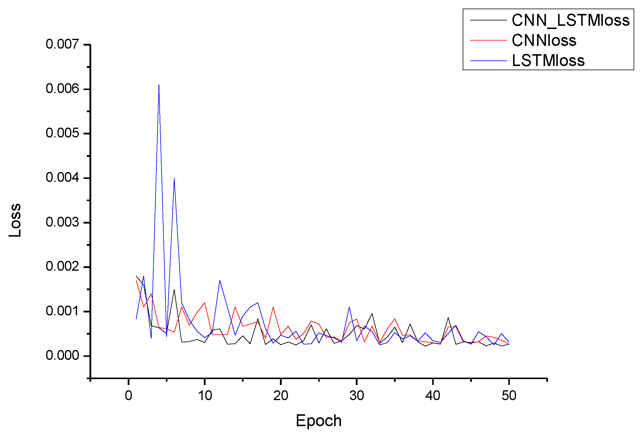
Since we achieved good results using the CNN-LSTM model, we used the idea of ablation to evaluate the impact of each module on performance. In the CNN-LSTM model, we removed the CNN layers or LSTM layers, both of which had a large impact on the performance of the system (the number of CNN layers changes also affected the final result). We selected the CNN model and the LSTM model for the model comparison. The CNN model was set with three layers of 1D-CNN (Filter = 64), the LSTM model was set with two layers of LSTM, and the time sliding window was 3. The optimizer was consistent with the CNN-LSTM model, and the Adam optimizer was selected. The loss function was MSE. When EPOCH was set to 50, CNN-LMST had the lowest loss and the best effect. This is shown in Figure 13 for specific values and in

Table 2. Performance in test data sets for each model.

Model	RMSE	MSE
LSTM	0.678	0.459
CNN	0.632	0.399
CNN-LSTM	0.623	0.388

. This model can be used for trajectory prediction of other motion units.

4. Discussion

In this paper, we proposed using a sun vector to calculate the ideal turntable position value. Then we took the ideal position value and turntable speed, current, and solar position error signal as date features and used the CNN-LSTM model to realize predicting the trajectory of the pitch axis. The model could adjust parameters adaptively on the training set and had a better performance on the test set.

The premise of the conventional feedback method is the need to calibrate the optical axis in relation to the instrument body coordinate system and the satellite coordinate system. The position of the pitch axis is then derived by determining the coefficients of the controller. The disadvantage is that certain parameters may need to be adjusted after a long period of system operation. The advantage is the high reliability due to the rigorous model derivation. The advantage of the deep learning method for calculating the pitch axis position is that it can be used without coordinate system calibration, allowing adaptive adjustment of the parameters. However, due to its black-box nature, this research is still at a preliminary stage for on-orbit applications.

Compared with the trajectory prediction method mentioned above, the pitch axis trajectory prediction of a two-dimensional turntable is a typical time series prediction problem [18,19]. It is not only related to the previous running state of the turntable but also is affected by the running state of a period of the time window. From this point of view, HMM and an extended Kalman filter only predict the next state through the last state, and the results will affect the accuracy of the prediction [20]. We did not use the equation of motion either, thereby avoiding uncertainty error analysis. We used a deep learning model to predict the trajectory by extracting and learning data features. We used a sliding time window instead of just the last state, and our findings were in accordance with recent studies indicating that a prediction model based on deep learning can achieve satisfactory results [21,22,23,24,25,26]. The prediction model based on the LSTM model could effectively avoid gradient disappearance or gradient explosion. In the process of debugging parameters, we also found that the initial value of parameters affected the final performance of the model. The size of the dataset also limited our choice of models. This model had a better performance on a small data set. For the comparison of the performance indicators of the LSTM model and CNN model alone, we could see that the sun vector combined with CNN-LSTM model had a better performance.

The major limitation of the present study was that the model contained part of the black box, so the model lacked interpretability. At the present stage, we mainly used the calculated results to compare with the real values and then used the comparison results to reverse-extrapolate to achieve the purpose of optimizing the performance of the model. The generalization ability of the CNN-LSTM model has yet to be verified. In addition, when the sliding time window becomes larger, the calculation time of the model will become longer. It will affect the execution time of the model.

Despite its limitations, the model of CNN-LSTM had a significant short-term prediction effect on turntable trajectory prediction.

Future applications in orbit will be different from the ground simulation. For the hardware environment, we must choose the processor to meet the onboard radiation—a hardened and tolerant processor generally using an ARM and field-programmable gate array (FPGA) fabric for real-time processing [27]. Software algorithms will be transplanted and optimized accordingly, and the trained network structure needs to be arranged on the onboard platform to work.

5. Conclusions

With the introduction of intelligent load and spaceborne integration, increasing attention has been paid to the problems related to two-dimensional turntable motion [28].

In this paper, different from the motion model and equation using traditional trajectory prediction, we used the sun vector and the CNN-LSTM model to predict the pitch axis position of the two-dimensional turntable. It had the advantages of adaptive adjustment of parameters and easier establishment of models. We calculated the ideal sun position through the sun vector model and input it into the model as a feature to participate in the prediction. Through comparison of performance indicators, the CNN-LSTM model combined with a solar vector model was superior to the LSTM model or the CNN model. The test results showed that the RMSE value was 0.623 and the MSE value was 0.388. The CNN-LSTM model could accurately predict the two-dimensional turntable operation.

This can be applied not only to track prediction of a turntable but also extended to other track predictions; for example, vehicle trajectory prediction, navigation trajectory prediction, etc. It also has broad prospects in other applications such as fault detection by predicting the state [29,30,31,32].

References

1. Chen, B.; Zhang, X.-X.; He, L.-P.; Song, K.-F.; Liu, S.-J.; Ding, G.-X.; Dun, J.-P.; Li, J.-W.; Li, Z.-H.; Guo, Q.-F.; et al. Solar X-ray and EUV imager on board the FY-3E satellite. Light. Sci. Appl. 2022, 11, 329. [Google Scholar] [CrossRef] [PubMed]
2. Wang, Z.; Huang, M.; Qian, L.; Zhao, B. Near-earth space two-dimension opto-electronic turntable design. Optik 2020, 200, 163387. [Google Scholar] [CrossRef]
3. Crassidis, J.L.; Alonso, R.; Junkins, J.L. Optimal Attitude and Position Determination from Line-of-Sight Measurements. J. Astronaut. Sci. 2000, 48, 391–408. [Google Scholar] [CrossRef]
4. Qiao, S.; Shen, D.; Wang, X.; Han, N.; Zhu, W. A Self-Adaptive Parameter Selection Trajectory Prediction Approach via Hidden Markov Models. IEEE Trans. Intell. Transp. Syst. 2014, 16, 284–296. [Google Scholar] [CrossRef]
5. Li, Q.; Li, R.; Ji, K.; Dai, W. Kalman filter and its application. In Proceedings of the 8th International Conference on Intelligent Networks and Intelligent Systems (ICINIS), Tianjin, China, 1–3 November 2015; IEEE: Piscataway, NJ, USA, 2015. [Google Scholar]
6. Zhou, Z.; Chen, J.; Shen, B.; Xiong, Z.; Shen, H.; Guo, F. A trajectory prediction method based on aircraft motion model and grey theory. In Proceedings of the 2016 IEEE Advanced Information Management, Communicates, Electronic and Automation Control Conference (IMCEC), Xi’an, China, 3–5 October 2016; IEEE: Piscataway, NJ, USA, 2016. [Google Scholar]
7. Wang, M.; Fu, W.; He, X.; Hao, S.; Wu, X. A survey on large-scale machine learning. IEEE Trans. Knowl. Data Eng. 2020, 34, 2574–2594. [Google Scholar] [CrossRef]
8. Zhou, H.; Chen, Y.; Zhang, S. Ship Trajectory Prediction Based on BP Neural Network. J. Artif. Intell. 2019, 1, 29–36. [Google Scholar] [CrossRef]
9. Zhou, H.; Zhang, S.; Peng, J.; Zhang, S.; Li, J.; Xiong, H.; Zhang, W. Informer: Beyond Efficient Transformer for Long Sequence Time-Series Forecasting. In Proceedings of the AAAI Conference on Artificial Intelligence, No. 23, Online, 2–9 February 2021; Volume 35. [Google Scholar]
10. Kuang, D.; Xu, B. Predicting kinetic triplets using a 1d convolutional neural network. Thermochim. Acta 2018, 669, 8–15. [Google Scholar] [CrossRef]
11. Yusoff, M.I.M.; Mohamed, I.; Bakar, M.R.A. Hidden Markov models: An insight. In Proceedings of the 6th International Conference on Information Technology and Multimedia, Putrajaya, Malaysia, 18–20 November 2014; IEEE: Piscataway, NJ, USA, 2014. [Google Scholar]
12. Qiao, S.J.; Wu, L.C.; Han, N.; Huang, F.L.; Mao, R.; Yuan, C.A.; Gutierrez, L.A. Multiple-motion-pattern Trajectory Prediction of Moving Objects with Context Awareness: A Survey. J. Softw. 2021, 34, 312–333. [Google Scholar]
13. Yu, F.X.; Zheng, Y.M.; Xie, C.X.; Jin, J.J.; Jin, Z.H. Error analysis of pico-satellite attitude angle measurement based on magnetometer. Jilin Daxue Xuebao 2007, 37, 1460. [Google Scholar]
14. Wertz, J.R. Spacecraft Attitude Determination and Control; Springer Science & Business Media: Berlin/Heidelberg, Germany, 2012; Volume 73. [Google Scholar]
15. Lecun, Y.; Bottou, L.; Bengio, Y.; Haffner, P. Gradient-based learning applied to document recognition. Proc. IEEE 1998, 86, 2278–2324. [Google Scholar] [CrossRef] [Green Version]
16. Sepp, H.; Schmidhuber, J. Long short-term memory. Neural Comput. 1997, 9, 1735–1780. [Google Scholar]
17. Kingma, D.P.; Ba, J. Adam: A method for stochastic optimization. arXiv 2014, arXiv:1412.6980. [Google Scholar]
18. Montgomery, D.C.; Jennings, C.L.; Kulahci, M. Introduction to Time series Analysis and Forecasting; John Wiley & Sons: Hoboken, NJ, USA, 2015. [Google Scholar]
19. Horvatic, D.; Stanley, H.E.; Podobnik, B. Detrended cross-correlation analysis for non-stationary time series with periodic trends. Europhys. Lett. 2011, 94, 18007. [Google Scholar] [CrossRef] [Green Version]
20. He, W.; Williard, N.; Chen, C.; Pecht, M. State of charge estimation for electric vehicle batteries using unscented kalman filtering. Microelectron. Reliab. 2013, 53, 840–847. [Google Scholar] [CrossRef]
21. Chemali, E.; Kollmeyer, P.J.; Preindl, M.; Emadi, A. State-of-charge estimation of Li-ion batteries using deep neural networks: A machine learning approach. J. Power Sources 2018, 400, 242–255. [Google Scholar] [CrossRef]
22. Lee, J.-Y.; Jo, B.-U.; Moon, G.-H.; Tahk, M.-J.; Ahn, J. Intercept Point Prediction of Ballistic Missile Defense Using Neural Network Learning. Int. J. Aeronaut. Space Sci. 2020, 21, 1092–1104. [Google Scholar] [CrossRef]
23. Baccouche, M.; Mamalet, F.; Wolf, C.; Garcia, C.; Baskurt, A. Sequential deep learning for human action recognition. In Human Behavior Understanding, Proceedings of the Second International Workshop, HBU 2011, Amsterdam, The Netherlands, 16 November 2011; Proceedings 2; Springer: Berlin/Heidelberg, Germany, 2011. [Google Scholar]
24. Sutskever; Ilya; Vinyals, O.; Le, Q.V. Sequence to sequence learning with neural networks. In Proceedings of the Advances in Neural Information Processing Systems 27: Annual Conference on Neural Information Processing Systems 2014, Montreal, QC, Canada, 8–13 December 2014; Volume 27. [Google Scholar]
25. Guo, L.; Lei, Y.; Xing, S.; Yan, T.; Li, N. Deep Convolutional Transfer Learning Network: A New Method for Intelligent Fault Diagnosis of Machines with Unlabeled Data. IEEE Trans. Ind. Electron. 2019, 66, 7316–7325. [Google Scholar] [CrossRef]
26. Tang, Y.; Dou, L.; Zhang, R.; Zhang, X.; Liu, W. Deep Transfer Learning-based Fault Diagnosis of Spacecraft Attitude System. In Proceedings of the 39th Chinese Control Conference (CCC), Shenyang, China, 27–29 July 2020. [Google Scholar]
27. Mandl, D.J. Real-Time Data Products and the Intelligent Payload Module. In Proceedings of the HyspIRI and Surface Biology and Geology Science and Applications Workshop, Washington, DC, USA, 15–17 August 2018. No. GSFC-E-DAA-TN60324. [Google Scholar]
28. You, Z.; Wang, C.; Xing, F.; Sun, T. Key technologies of smart optical payload in space remote sensing. Spacecr. Recovery Remote Sens. 2013, 34, 35–43. [Google Scholar]
29. Liu, B.; Yan, S.; Li, J.; Qu, G.; Li, Y.; Lang, J.; Gu, R. A Sequence-to-Sequence Air Quality Predictor Based on the n-Step Recurrent Prediction. IEEE Access 2019, 7, 43331–43345. [Google Scholar] [CrossRef]
30. Zhou, Y.; Dong, M.; Wu, J. Hyperparameter Optimization for SOC Estimation by LSTM with Internal Resistance. In Proceedings of the 2021 International Conference on Computer Network, Electronic and Automation (ICCNEA), Xi’an, China, 24–26 September 2021; IEEE: Piscataway, NJ, USA, 2021. [Google Scholar]
31. Zhou, X.; Shi, J.; Gong, K.; Zhu, C.; Hua, J.; Xu, J. A Novel Quench Detection Method Based on CNN-LSTM Model. IEEE Trans. Appl. Supercond. 2021, 31, 4702105. [Google Scholar] [CrossRef]
32. Fu, J.; Sun, C.; Yu, Z.; Liu, L. A hybrid CNN-LSTM model based actuator fault diagnosis for six-rotor UAVs. In Proceedings of the 2019 Chinese Control and Decision Conference (CCDC), Nanchang, China, 3–5 June 2019; pp. 410–414. [Google Scholar] [CrossRef]
Figure 1. Schematic diagram of the position of the sun, satellite, and turntable. (a) Schematic diagram of satellite orbit, and sun is in −Y direction. (b) Turntable optical axis coordinate system.
Applsci 13 04939 g001
Figure 2. Solar images obtained by X-EUVI when the optical axis points to the sun (from the National Meteorological Satellite Center of China).
Applsci 13 04939 g002
Figure 3. The 1D-CNN model structure, the blue color parts represents processing dot product with input slide window part and kernel.
Applsci 13 04939 g003
Figure 4. LSTM model structure.
Applsci 13 04939 g004
Figure 5. Proposed CNN-LSTM model architecture with input sequence, two CNNs layer, an LSTM layer, a dropout layer, dense layer, and an output.
Applsci 13 04939 g005
Figure 6. CNN-LSTM model operation diagram, the yellow parts represent the layer of CNN, and the green parts represent the layer of LSTM.
Applsci 13 04939 g006
Figure 7. Proposed CNN-LSTM, model architecture parameter.
Applsci 13 04939 g007
Figure 8. Prediction processing.
Applsci 13 04939 g008
Figure 9. Data feature curves of pitch axis.
Applsci 13 04939 g009
Figure 10. True position curve of pitch axis from data set.
Applsci 13 04939 g010
Figure 11. Loss curve for training set and test set.
Applsci 13 04939 g011
Figure 12. Forecast location map for test set.
Applsci 13 04939 g012
Figure 13. Loss diagram of each model for the test set.
Applsci 13 04939 g013