1. Introduction
At present, rare earth elements, energy resources, and novel materials hold considerable value around the world. Graphite products, as well as a broad spectrum of downstream extensively processed commodities, are attracting growing attention and have become an essential, irreplaceable component in crucial sectors, such as national security, space exploration, and novel materials. However, conventional methods for identifying the grade of carbon content of graphite ore through chemical or physical tests lead to resource wastage and low efficiency during the ore blending process. With the steady advancement and stability of computer hardware, the use of equipment, such as Graphics Processing Units (GPUs), has become widespread [
1], and deep learning has made significant progress in target recognition and image classification [
2]. Moshayedi et al. [
3] employed deep learning techniques and drones placed at low altitudes to detect real-time vehicle speeds in the city, thus ensuring security for future unmanned smart cities. Sun X et al. [
4] improved the Faster Region Convolutional Neural Network (Faster R-CNN) with feature splicing, hard negative mining, and multi-scale training, achieving notable results in face detection. Furthermore, Albahli S et al. [
5] introduced DenseNet-41 to the Faster R-CNN model, calculating deep features that yielded better application outcomes in handwritten digit recognition.
Furlán and colleagues (2019) employed convolutional neural networks, a sophisticated class of deep learning algorithms, to discern rock types bearing resemblance to those indigenous to the red planet, Mars. This research endeavor was further supported by the effective deployment of a comprehensive and diverse dataset comprised of multiple Martian-like images [
6].
Meanwhile, Zhao et al. (2020) utilized the improved YOLOv3 algorithm to enhance target detection accuracy [
7].
In a scholarly investigation conducted by Xu et al. (2020), a comparative analysis was undertaken between the utilization of YOLOv4 and Faster R-CNN models for the purpose of rock category detection. The outcome of the investigation revealed that the latter model exhibited greater accuracy in its detection performance. Furthermore, in a distinct research study [
8], the aforementioned models were evaluated and contrasted based on their respective capabilities to discern objects within images, with results indicating that the Faster R-CNN model yielded more precise outcomes.
Zhang et al. (2018) [
9] have implemented the Mask R-CNN [
10] architecture for the swift identification of vehicular damage in the aftermath of traffic accidents. A comprehensive investigation into the current state-of-the-art methods of object detection reveals the pervasive deployment of deep learning frameworks, albeit with varying feature extraction network processes. The foundational Faster R-CNN network model [
11] has been subject to numerous modifications in its quest for more efficient performance, ranging from the utilization of lightweight models, such as MobileNet [
12], to more compact ones, such as VGGNet [
13] and ResNet [
14]. Such adaptations incorporate the residual module, which plays a crucial role in generating feature maps with a single layer that possesses relatively lower resolution.
To address the missed targets and the false detection of small targets and details after segmentation, this paper employs a multi-scale fusion approach to improve accuracy. Deep learning has gained significant attention from researchers across various fields for its ability to mimic human visual attention and its popularity in computer vision applications.
Prior notable algorithms include Squeeze-and-Excitation Networks (SE-Net) [
15], Selective Kernel Networks (SK-Net) [
16], and Convolutional Block Attention Module (CBAM) [
17]; of these, SE-Net is a channel-based network, SK-Net is a branch type network, and CBAM is a kind of hybrid method based on channel and spatial attention. However, in this paper, another network, the Relation-Aware Global Attention Network (RGA-Net) [
18], is based on relationship perception and pays more attention to global feature information. Compared to CBAM as the method that integrates channel and spatial attention, RGA has higher discrimination between foreground and background and can extract more effective information. In order to improve the model training effect and speed up the model training, most deep learning models currently use the Batch Normalization Layer (BN layer). However, in the training process, the BN layer depends on the batch size because it needs to calculate the intermediate statistics based on the batch, which can easily lead to inconsistency between training and testing results. So, in this paper, the BN layer changes into a Filter Response Normalization (FRN) layer [
19].
The main contributions of this paper are listed below:
- (1)
We proposed a novel model based on deep learning to identify the graphite ore grade quickly and conveniently.
- (2)
We proposed the image-cutting algorithm to build and enhance the datasets in the image database.
- (3)
Utilized image cutting to expand the dataset and combined it using the Feature Pyramid Networks (FPN) method to extract features.
- (4)
Proposed the Relation-Aware Global Attention (RGA) attention mechanism for the model pair that focuses more on the Region of Interest (ROI).
- (5)
Proposed the Filter Response Normalization (FRN) layer to fit with a small image batch size.
This article is divided into five different sections, each providing support for a comprehensive understanding of the model method we proposed. The Introduction section lays the foundation for subsequent sections by providing an overview of the topic under discussion.
Section 2 describes the detailed feature extraction process of the Faster R-CNN model.
Section 3 provides a detailed introduction to our approach and steps for improving the Faster R-CNN model.
Section 4 critically reviews the experiments and results of relevant research, comprehensively outlining the experimental design and methods used to validate the effectiveness of the model. Finally,
Section 5 provides a concise and persuasive conclusion that summarizes the main findings of the article and provides a glimpse into future research avenues.
2. Materials and Methods
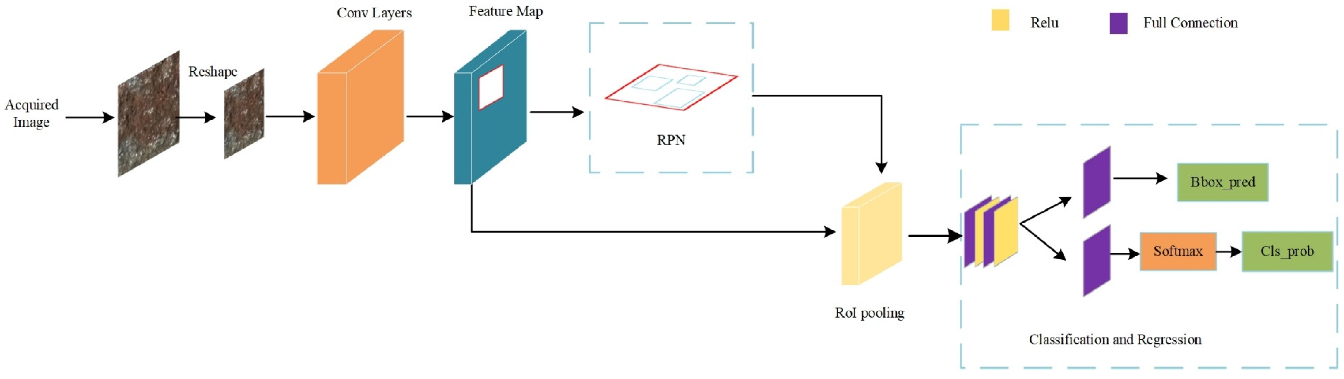
This section elaborates on the detailed feature extraction process of the Faster R-CNN (FR-CNN) model. The model description includes the deep learning model architecture, image dataset, convolution layer, RPN structure and mechanism, ROI pooling, and classification and regression operations. The deep learning model architecture refers to the multi-layer neural network used to identify complex patterns from input images. The image dataset is a collection of images for training and evaluation purposes, while the convolution layer extracts features from the input image. The RPN generates candidate regions, the ROI pooling aggregates features from these regions, and the classification and regression operations estimate object class and refine bounding box coordinates. Finally, the proposal boxes are obtained, and the classification and regression operations identify and localize objects of interest.
2.1. Deep Learning Model Architecture
The FR-CNN is a two-stage object detection network model proposed by Shaoqing Ren et al. [
11] in 2015. This model also can work as a single, end-to-end deep convolutional neural network for object detection and evolved from Region CNN (R-CNN) [
20] and Fast Region CNN (Fast R-CNN) [
21] network models. However, R-CNN relies on the Selective Search algorithm to generate a region proposal network, which takes a lot of time and cost; Fast R-CNN has made a series of improvements to the R-CNN model, the most important of which is to propose the Region of Interest (ROI) Pooling layer. It can extract feature vectors of equal length from all regions of interest (i.e., ROI) in the same image, which can effectively avoid the need for R-CNN to segment and deform the image to meet the input size of the image before performing the convolution operation. Concerning the feature loss, FR-CNN retains the advantages of the previous two methods (R-CNN, Fast R-CNN) and introduces the region proposal generation network Region Proposal Network (RPN) based on Fast R-CNN. In addition, it should be noted that R-CNN and Fast R-CNN models rely on selective search algorithms to generate proposal regions. While Region Proposal Network (RPN) in Faster R-CNN can use the same convolutional layers to process images, Faster R-CNN does not need to spend extra time generating proposals. Then, FR-CNN detection time is greatly shortened, and the accuracy rate is also improved to a certain extent. The structure of the FR-CNN model is shown in
Figure 1.
The initial step in the processing pipeline involves reshaping the raw graphite ore image to conform to the input size specifications of the backbone extraction network residing in the Convolutional Layers. The backbone extraction network, subsequently, engages in the extraction of essential features from the reshaped image through a series of computational operations. Once the feature map has been generated, it is then directed to the Regional Proposal Generation Network (RPN), which is responsible for generating a proposal frame that encapsulates the target object within the image. Subsequently, the proposal frame and the feature map are transmitted to RoI Pooling, which performs a pooling operation on the feature map to crop out the proposal frame, thus generating a fixed-size rectangular box. Finally, the feature map within the rectangular box undergoes classification and regression predictions through full connection to yield the desired output.
2.2. Image Dataset
The section dedicated to the dataset is contingent upon the acquisition of bona fide imagery and meticulous annotation techniques, which are elucidated in detail in the ensuing exposition.
2.2.1. Images Acquisition
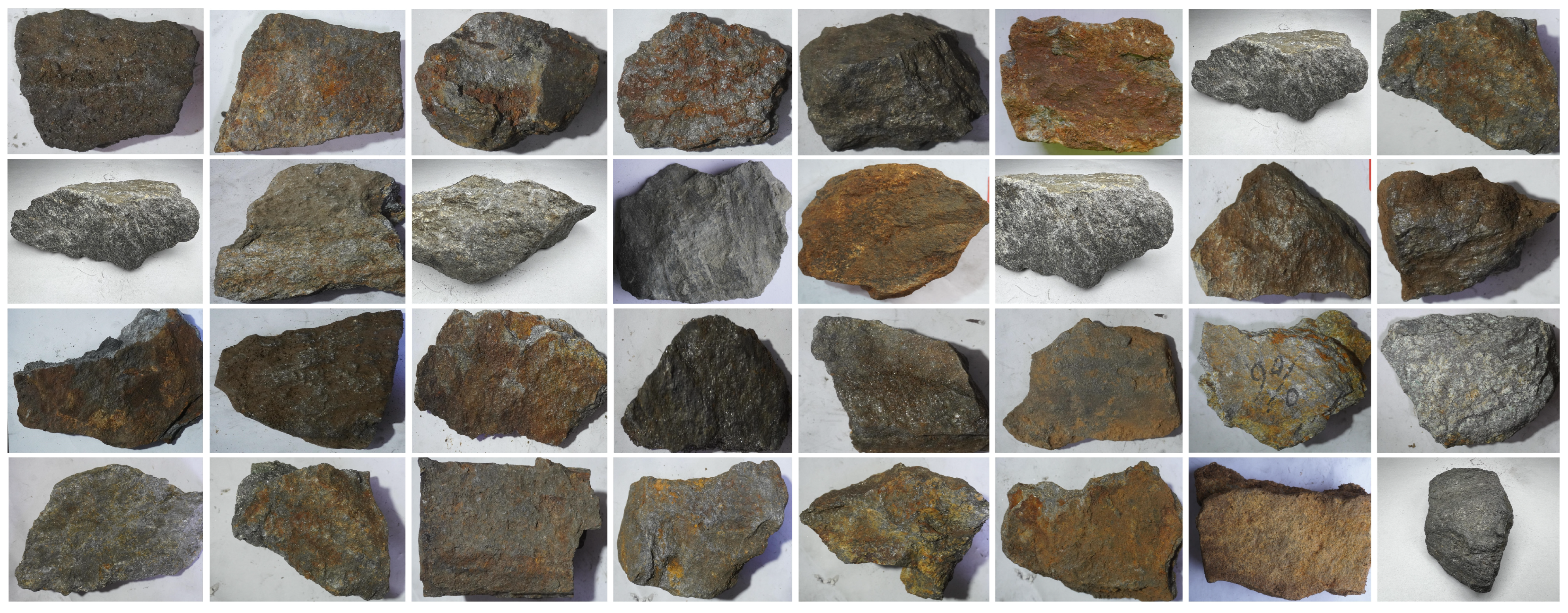
The present study employed an image dataset that was sourced from the graphite mine field laboratory. The entire corpus of photographic samples was captured using a Canon EOS 5D Mark II camera. The authentic stone specimens utilized in this research were obtained from the mines situated in the Heilongjiang Province of China. Based on the expert evaluation, it can be stated that the carbon content of graphite ore is typically not more than 20%. The primary image data, obtained from the experiment, have been depicted in
Figure 2.
As illustrated in
Figure 2, with respect to the upper limit of ore concentration in the samples, namely 20%, the samples are classified into four distinct categories ranging from 0 to 5%, 5 to 10%, 10 to 15%, and 15 to 20%. This classification serves the purpose of indicating the carbon content, as presented in
Table 1. However, due to the scarcity of image datasets and significant variations in the number and proportion of carbon content images across different stages, effectively training the model has become a challenging task, leading to unsatisfactory outcomes. In light of these constraints, this research puts forth a novel approach, involving an image-cutting algorithm, to augment the available data. The proposed algorithm divides each image into multiple images of equal dimensions in accordance with specific aspect ratios.
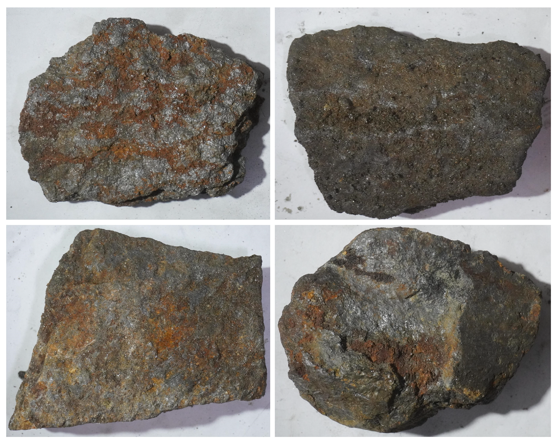
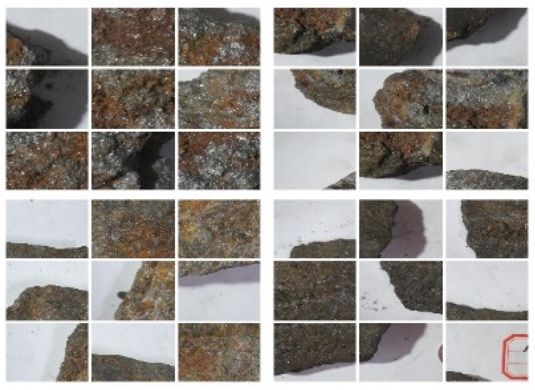
This study employs a rigorous approach to image processing by employing high-resolution images with a resolution of 1024 × 1024 pixels for all the training, validation, and testing datasets. Notably, the initial number of segments for each image data differs, and, consequently, the specific ratio of segments varies depending on the number of images in each segment, as graphically illustrated in
Figure 3 and
Figure 4.
Figure 3 and
Figure 4 show the original graphite ore image and the schematic diagram after cutting.
2.2.2. Images Annotation
To utilize the dataset for the purpose of model training, the subsequent course of action entails the utilization of the image labeling tool, Labelme [
22], for the purpose of demarcating the sliced graphite ore images. Subsequently, the dataset is partitioned into three distinct components, namely, the training set, the validation set, and the test set, with a distribution ratio of 6:2:2, respectively. The resulting distribution of the image dataset is depicted in
Table 1.
Table 1 illustrates that the partitioned image dataset quantities for each of the groups (G1 through G4) exhibit variation. The sample sizes of Group 1 to Group 4 are approximately equal. A segmentation algorithm is used to further divide each group into smaller samples of equal size, and then according to a predetermined ratio, evenly partitioned into experimental dataset, training dataset, validation dataset, and testing dataset.
2.2.3. Image Reshape
To follow the input size requirement of the CNN feature extraction network, the reshape operation needs to be performed before the original image enters the feature extraction stage.
2.3. Convolution Layer
The convolution layer section consists of image feature extraction and trunk extraction network principle and introduction. The following describes a detailed image extraction method step-by-step in order to extract useful information.
2.3.1. Image Feature Extraction
This section consists of the most basic unit structure of the feature extraction network and the complete structure of the entire network, and the main aim of this section is to introduce the working mechanism of the feature extraction network from simple to complex.
2.3.2. Trunk Extraction Network Principle and Introduction
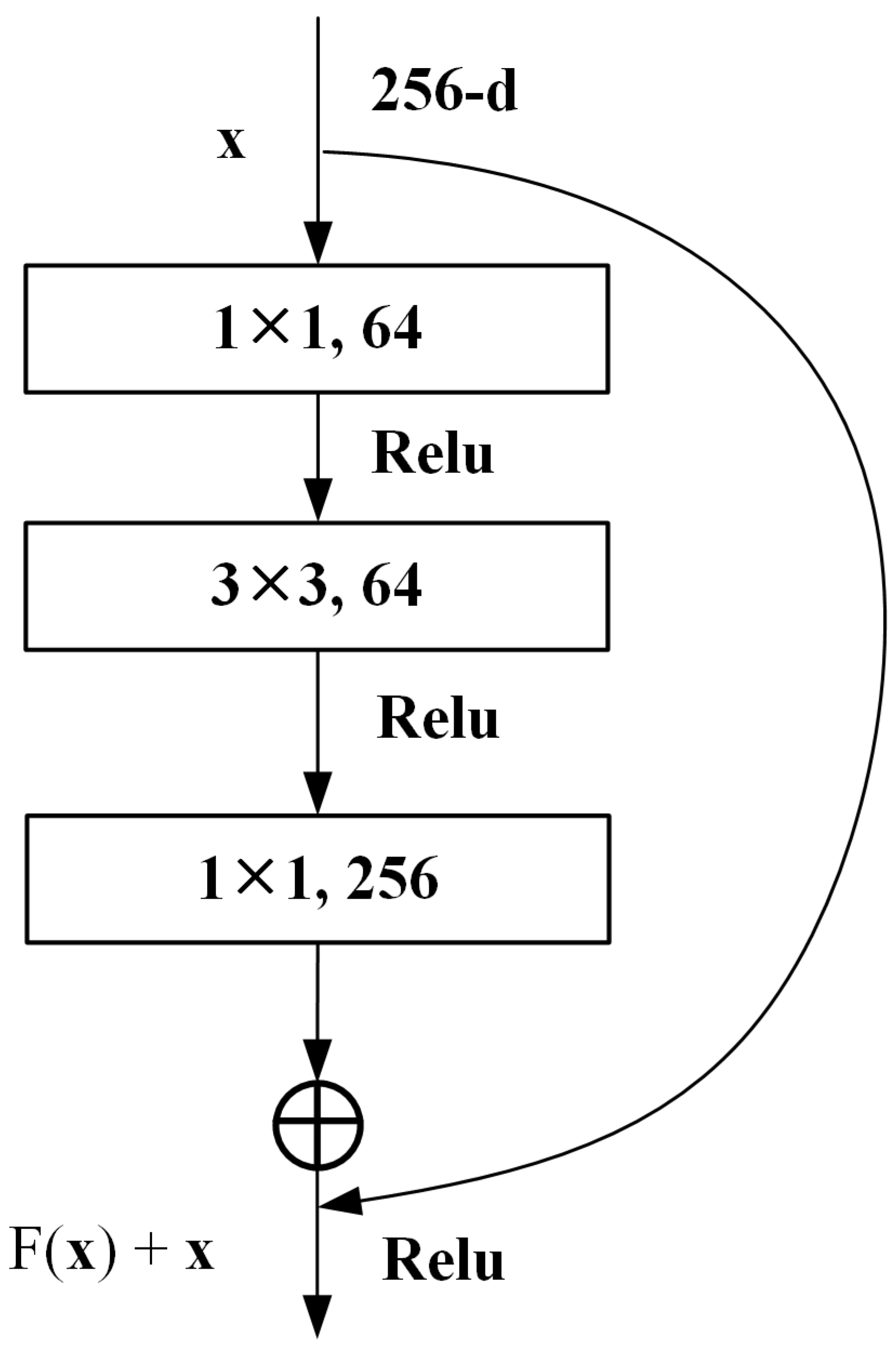
In this research, the backbone extraction network selected is ResNet50, a residual network constructed by several blocks. The basic residual block is shown in
Figure 5.
The basic residual network (
Figure 5) shows that the structure can be split into the main area and the side area. First, the preprocessed graphite ore images is input as a feature matrix into the residual structure for feature extraction, it is designated as 256-d. With the next convolution layer, with the dimension of 1 × 1 × 64, the number of channels becomes 64; after the activation function ReLu, a 3 × 3 × 64 convolution layer is passed, and the number of channels remains unchanged at this time; in a 1 × 1 × 256 convolutional layer, at this time, the number of input channels becomes 256, and then adding the outputs of the main branch and sub-branch leads to obtain the output of the residual block. This can reduce the number of parameters, reduce the amount of calculation, and effectively improve the network’s depth. The final output of this residual block is shown in Equation (1).
In Equation (1),
represents the input of the basic residual block.
represents the network map before summation. The exact structure of ResNet50, composed of basic residual blocks, is shown in
Table 2.
As shown in
Table 2, the primary step entails acquiring the input image via the 7 × 7 × 64 convolutional layers, Conv1, followed by the application of the 3 × 3 max pool and a sequence of convolutional blocks from Conv2_x to Conv5_x. Subsequently, the final output is obtained through a 1 × 1 Average pool, FC, and Softmax [
23]. In comparison with other networks, ResNet50 evades the gradient disappearance and gradient explosion issues that arise during the deep learning process and resolves the network degradation problem prevalent in deep learning training processes. For this experiment, the 50-layer network architecture of the ResNet series was selected to yield superior results.
2.4. Region Proposal Network (RPN)
The significance of the existence of the RPN network is to extract the pre-selected box as part of the R-CNN [
20] that uses the selective search algorithm for Region Proposal. In RCNN and Fast-RCNN [
21], there is a bottleneck process in extracting pre-selected boxes. Because RPN introduces a convolutional network, which makes the pre-selected feature extraction form to generate the position of the box, thereby it causes the reduction of the impact of selective search algorithms and the computational time overhead. Therefore, RPN can significantly improve performance. The proposal box sections extraction consists of the RPN structure and mechanism. The RPN processing and loss calculation function is described as follows.
2.4.1. RPN Structure and Mechanism
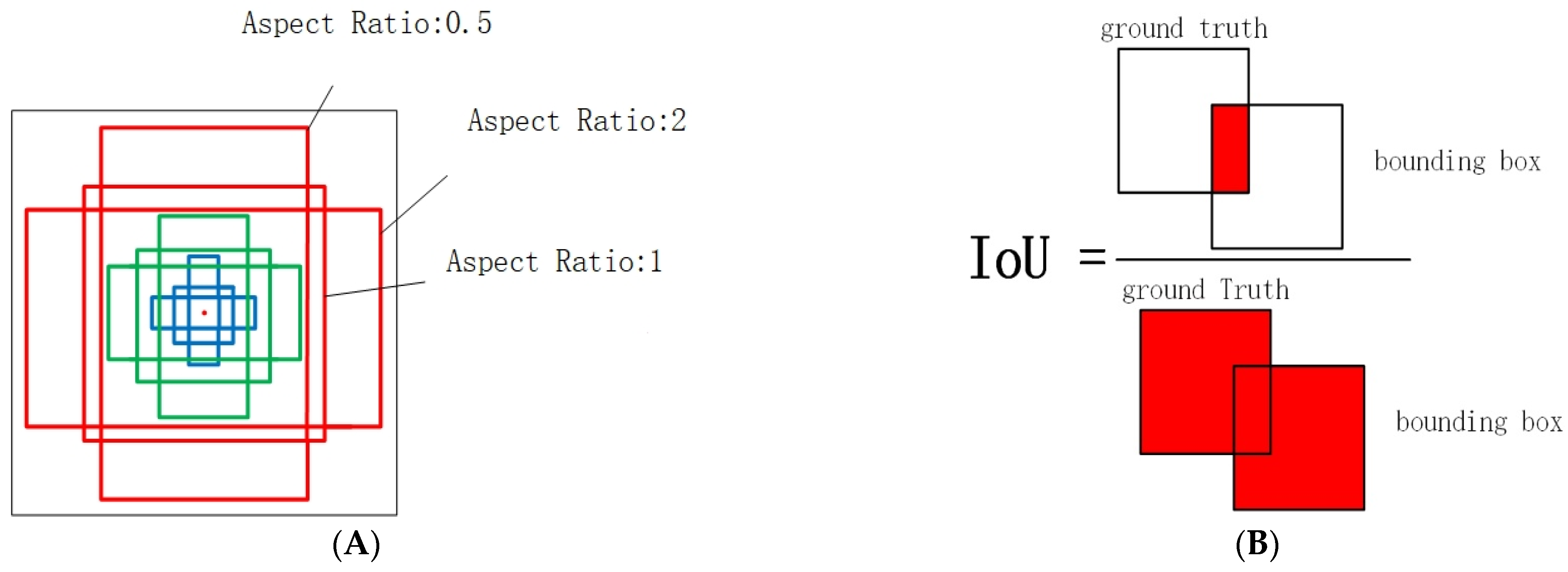
The input of the RPN is the feature map generated by the feature extraction layer, and 9 anchors are defined on each pixel of the feature map, corresponding to 3 scales (128, 256, 512) and aspect ratio (0.5, 1, 2). The schematic diagram of 9 different anchors is shown in
Figure 6.
As it is shown in
Figure 6A, at each pixel (C, H, W) of the feature map, (H/16) × (W/16) × 9 anchors are generated, and there are about 20,000 anchors. It will be very time-consuming to generate more than 20,000 anchors to participate in the calculation, and there are too many negative samples, and the final effect is not ideal. Therefore, under the action of the anchor target generator, according to the IoU of the anchor and the real box, 256 anchors are selected as the total samples during training. The calculation method of IoU represents the true red box and the predicted red box represents the ratio of intersection and union, as shown in
Figure 6B. Taking the current pixel as the centre, according to 9 anchors of predefined size and aspect ratio. It represents ymin, xmin, ymax, and xmax multiplied by the corresponding ratio to calculate the position of each pixel on the output feature map corresponding to the original image (
Figure 7).
2.4.2. RPN Processing
As
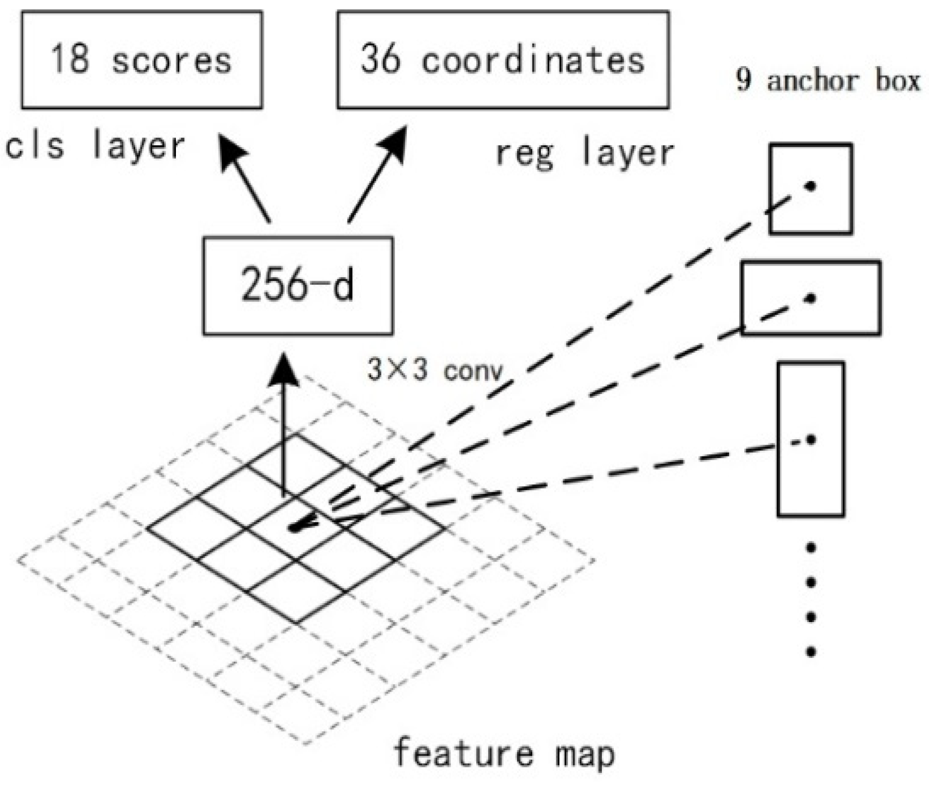
Figure 7 shows, the feature map performs a 256 × 3 × 3 convolution operation with each pixel as the centre to extract candidate regions, and the dimension of the input feature map is changed to 256. Next, two 1 × 1 convolution operations are performed, and finally, the classification result and the frame regression result are obtained. The principle of RPN is shown in
Figure 8. There are 9 anchor boxes in this paper. Therefore, RPN performs 3 × 3 at a certain window position. After the 1×1 convolution operation, the convolution outputs dimensions of 2 × 9 (18) and 4 × 9 (36) will be obtained, respectively. The output 18-dimensional branch will classify the foreground and background; the 36-dimensional branch is the bounding box regression coordinate, and the anchor points are adjusted to fit the predicted target better.
2.4.3. Loss Calculation Function
The loss function of RPN consists of two parts: the classification loss and the regression loss, and the summation of them is considered as the loss value of the RPN, as shown in Equation (2).
Based on Equation (2), the first term represents the classification loss part, which is used to decide whether it is a positive sample. Additionally, since it does not need a positive sample-dependent category classification, it uses the cross-entropy loss function for binary classification. In Equation (2),
and are the normalization; is constant with the default value of 10.
The loss function classification formula (first term) is shown in Equation (3).
In Equation (3), indicated the probability and shows the predicted label of the ith positive anchor sample; based on this formula, if is a positive sample, it is equal to one, (), otherwise, it has zero value ().
As the second term in Equation (2),
is used to keep the losses balanced between the two parts. In the case that there is no foreground and background within the detection anchor, the value is set to 0
; and in other cases, it is the reciprocal of the sum of foreground and background. The term
in the classification prediction also appears in the regression loss part, which ensures that non-positive samples generate regression loss. This paper calculated the regression loss using Smooth L1 Loss [
21], represented by a piecewise function form combining linear and quadratic functions [
24]. Using the quadratic function with the bases between (−1, 1) causes the image function to become smoothly near the zero point. However, it should be mentioned that the divergence is not easy for large forecast biases. In the next Equation, the calculation of the regression loss function is shown in Equations (4) and (5).
In Equation (4), represents the predicted position of the anchor, and represents the location of the real sample. For , as the input of the function, there are two cases. When the range of is (−1, 1), is the first in Equation (5); in other cases, the expression for is the second in Equation (5).
2.5. Region of Interest Pooling (RoI Pooling)
In conventional convolutional neural networks (CNNs), such as Visual Geometry Group (VGG) or AlexNet [
25], the input size is fixed during training [
26]. Any deviation from the fixed input size renders the network unsuitable for feature extraction. To overcome this issue, two methods have been employed by traditional networks, image cropping and image resizing. However, both methods result in a loss of original image information. To address this problem, RoI Pooling was introduced. This method avoids feature extraction for each proposal and instead extracts the RoI feature area from the original feature map through mapping. The input to RoI Pooling comprises of proposal box outputs generated by the RPN, namely ROIs, and feature maps of the entire image. Based on the input image, the RoI is mapped to the corresponding feature map position, the mapped area is then partitioned into regions of equal size, and a max pooling operation is subsequently performed on each region.
2.6. Classification and Regression
Feature maps will enter the Classification and Regression section after being processed by the RoI Pooling layer. In this part, proposal feature maps will obtain the position offset of each proposal, here we define them as Bbox_pred, through Full Connection; proposal feature maps will obtain the specific category Cls_prob of each proposal through Full Connection and Softmax at the same time.
3. Proposed Novel FRCNN-PGR Model
The FRCNN-PGR model is improved based on the FR-CNN model and innovatively integrates Feature Pyramid Networks, Relation-Aware Global Attention, and Filter Response Normalization, so this research is named FRCNN-PGR and described in the following subsections.
3.1. Models That Fuse Multi-Scale Features
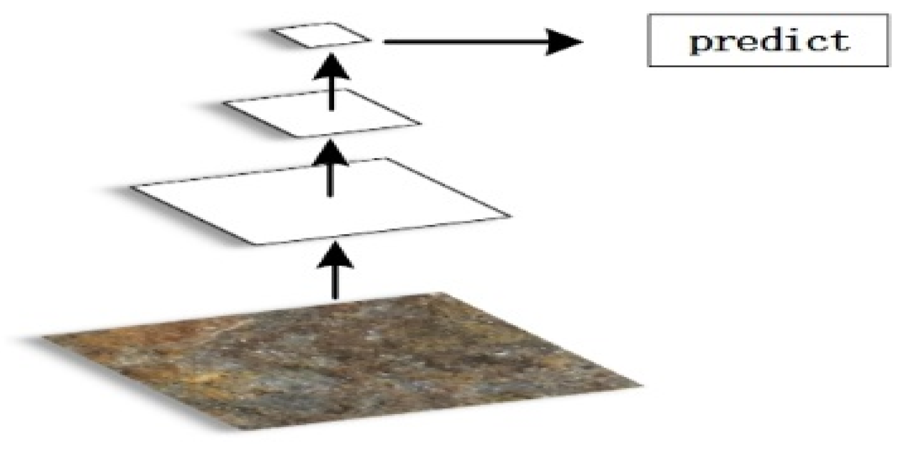
In this paper, the graphite ore images are cut multiple times, and there are large differences in the size of the positive samples in the images. Some ore images have a large quantity (Area), while others have a very small proportion of ore. The FR-CNN algorithm model continuously extracts image features under the deep convolutional neural network. After layering by layer convolution, the image will gradually lose some detailed information, which will cause the model to predict small objects and details inaccurately. Single feature extraction is shown in
Figure 8.
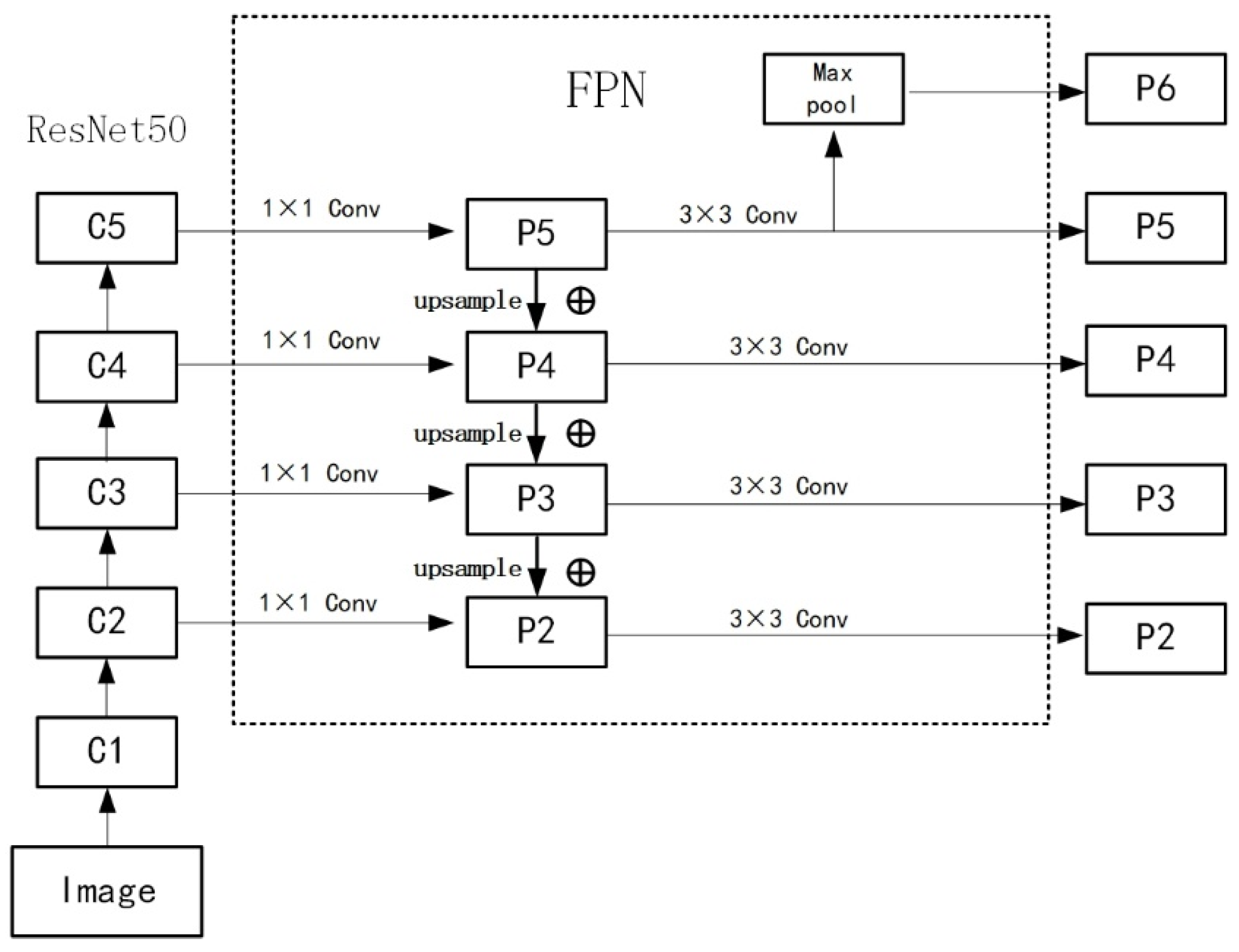
Figure 8 shows that the size of the feature map decreases as the network depth increases, and only the top-level features are used for prediction. Therefore, this paper adds Feature Pyramid Network (FPN) [
27] to the backbone feature extraction network. The structure of the combination of feature maps at different levels is shown in
Figure 9.
Figure 9 shows the performance of a 1 × 1 convolution operation on the four feature extraction convolution blocks of the ResNet50 network. Then, in this structure, the number of channels in each convolution layer can be the same to facilitate subsequent operations, upsample the high-level feature map after changing the channel and adding a shallow layer feature, and then go through a 3 × 3 convolution to complete the entire FPN process. The final feature map fuses high-level and low-level features, bringing ideal results to graphite ore images’ detailed texture and small target recognition.
3.2. RGA Global Attention Mechanism
The attention mechanism originally imitated the method of human thought that is applied to some natural language processing problems, and solved language translation or reasoning that depended on the context. The method has recently been widely used in deep learning-related problems. Through the attention mechanism, we can pay attention to the parts we are interested in and suppress the information we do not need. Previously, the local convolution method was usually used to learn the attention weight, and the feature information of the global structure was not considered [
28]. Then, this paper adds a global attention mechanism, RGA [
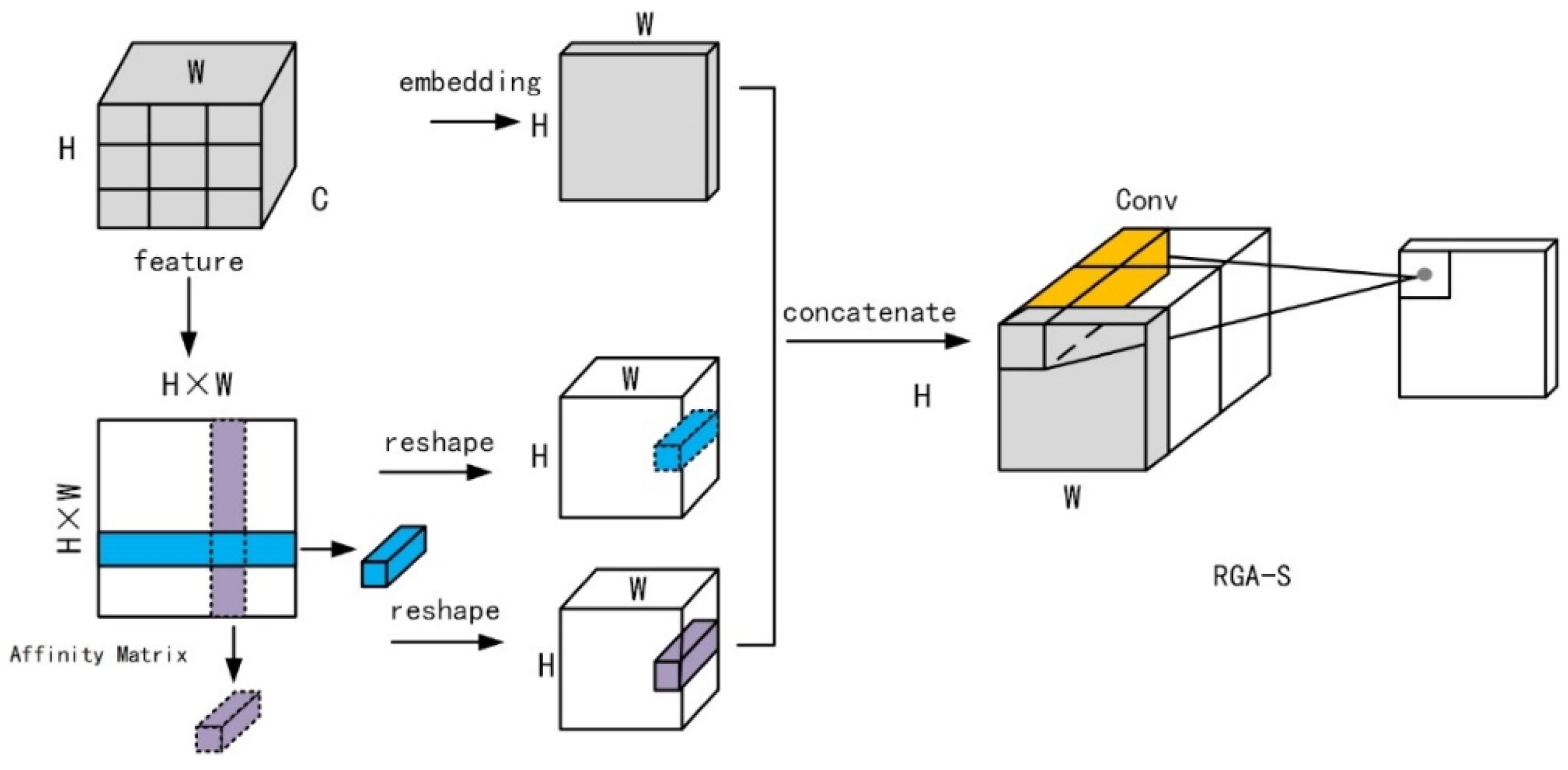
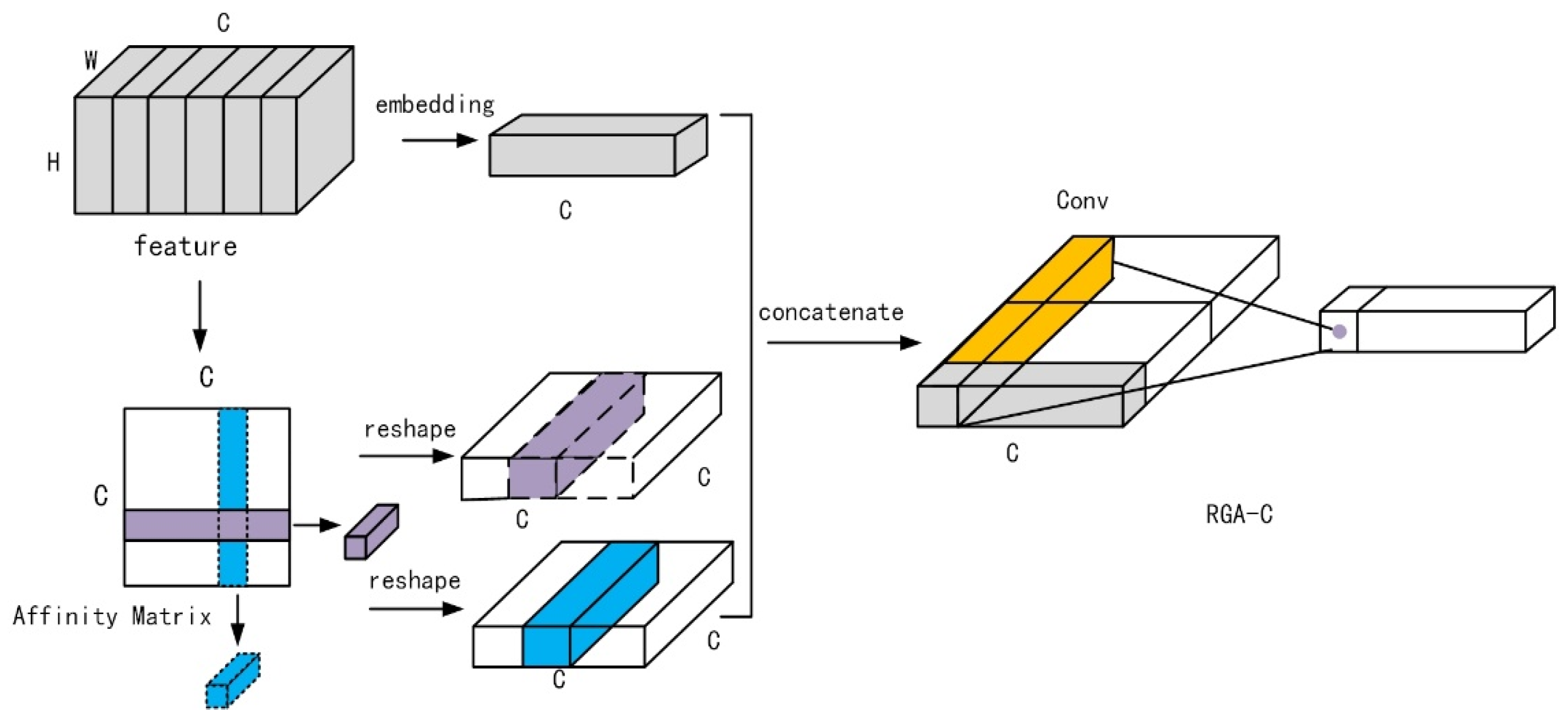
18], to the residual structure. The RGA attention mechanism consists of spatial and channel levels, namely RGA-S and RGA-C, as shown in
Figure 10 and
Figure 11 and concerning
Table 2. This paper adds RGA-S and RGA-C after each convolution block of Conv2_x to Conv5_x of the residual network ResNet50. Although this will increase the amount of calculation required, it can maximize the feature. However, the extraction has a good effect, and the increased time will not greatly impact the detection.
The two parts of the RGA structure extend the feature nodes along the spatial direction and the channel direction, respectively, and the Affinity Matrix is calculated to represent the correlation between the features. The correlation can be expressed by Equation (6)
where
and
are showing the two different features. The functions
and
are the sum of 1 × 1 convolution, BN, and activation function ReLU. They also reshape the Affinity Matrix along the horizontal and vertical directions to obtain two sets of features representing a pair of correlations. Once again, through 1 × 1 convolution, BN, and activation function ReLU, the original feature and the correlation vector can be mapped to the same feature domain, and, through the splicing operation, they are turned into a new attention feature structure. Finally, a set of spatial and channel attention weights are obtained, respectively.
3.3. Filter Response Normalization (FRN)
In the normalization method, Batch Normalization (BN) normalized the output of each neural network layer. BN can speed up the training speed of the model network and make the model converge faster and effectively reduce the possibility of gradient explosion. On the other side, the gradient disappearance can also prevent model training from overfitting. However, the BN layer is more suitable for large batches, and due to hardware limitations, the batch size set in this paper is small during training, so the FRN layer is introduced.
FRN and BN have the same effect, but FRN performs better on large or small batches. Singh et al. [
19] comparative experiments were conducted on FRN, GN [
29], and BN. He used the InceptionV3 [
30] and ResnetV2-50 [
31] models to classify the ImageNet dataset. He found that under the same experimental conditions, the model using the FRN layer performed better than the BN layer, with an improvement of approximately 1%. Additionally, by further reducing the Batch Size, the model with the FRN layer outperformed the GN layer on the same problem. Finally, he tested the model on the COCO dataset, and the experimental results showed that the FRN layer exhibited stable performance in both large and small Batch Sizes, with an improvement of 0.3% to 0.5% over other methods. The FRN layer structure is shown in
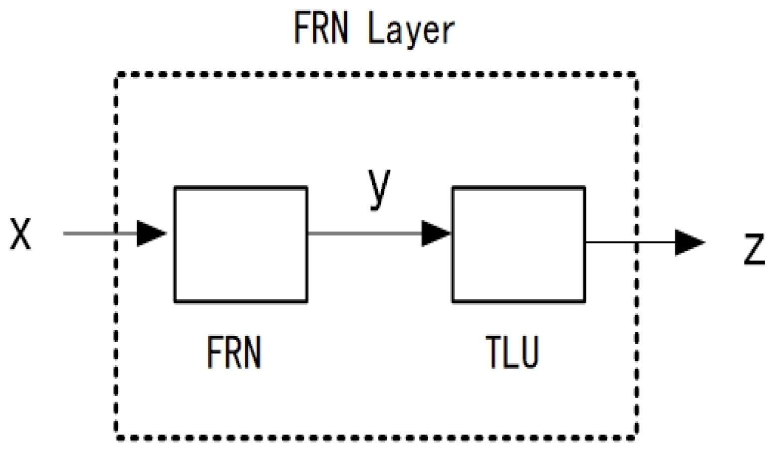
Figure 12.
As is shown in
Figure 12, the FRN layer consists of two parts, Filter Response Normalization (FRN) and Threshold Linear Unit (TLU).
- (1)
The Filter Response Normalized (FRN) formula is represented in Equations (7)–(9).
In Equation (7), , the form of vector is [B, H, W, C]; [B, H, W, C] is the input tensor of shape. The expression of only contains W and H, and FRN is not affected by the batch size. The represents the value of Mean square norm; in Equation (8) is a small normal quantity, which is used to prevent the dividend, that is, the denominator, from being zero; the calculation result expression is shown in Equation (9), where and are both learnable parameters.
- (2)
Threshold Linear Unit (TLU): The lack of mean centre in FRN may cause the activation to be any deviation from zero; such deviation combined with ReLU will bring a bad effect.
Therefore, when using FRN, it is often combined with TLU. The calculation of TLU is shown in the Equation (10).
where
represents the output of the FRN in Equation (9);
represents a learnable threshold. TLU uses the learning threshold
based on ReLU to solve the problem of arbitrary deviation in FRN without the mean centre.
4. Experimental Results and Analysis
This study utilizes the Windows 10 operating system, with an Nvidia GeForce RTX A4000 GPU and a 6-core Intel (R) Xeon (R) Silver 4310 CPU @ 2.10GHz processor, coupled with the pytorch1.10.0 deep learning framework. The pre-trained weights of the model are also incorporated into the experiment. The dataset under consideration comprises 1399 images of graphite ore that have been augmented and segregated by us into three portions, allocated for model training, verification, and testing, with a ratio of 6:2:2. A detailed illustration of the dataset is depicted in
Figure 1 (Image Acquisition and Annotation). Regarding the training parameter settings, we configured each batch to contain 8 images, and the initial learning rate (LR) was set at 0.01. The momentum parameter of SGD was assigned a value of 0.09, and the maximum number of training rounds is 100, with the training process ceasing when the model attains convergence. We employed transfer learning to expedite the training procedure.
4.1. Evaluation Criteria
To evaluate the efficacy of the FRCNN-PGR model, this scholarly manuscript employs the average precision (AP) metric to assess the detection outcomes within distinct grade ranges, and the mean average precision (mAP) to evaluate the overall average AP of all the grade categories, thus embodying the model’s predictions. Furthermore, the enhanced model is appraised using Recall (R) as a metric to compute the model’s recall rate. Moreover, the performance of the model is further assessed by utilizing the false positive rate (FPR) and false negative rate (FNR) metrics.
The definition of precision is shown in Equation (11), where
indicates the number of the predicted samples is indeed true, and FP indicates that the predictor judges’ false samples as true.
represents all samples predicted by the model (detected by the model). The Recall is defined in Equation (12)
where
has the same meaning as
in precision,
means all true samples (model detected and not detected). The FPR and FNR are defined in Equations (13) and (14).
In Equation (13), represents the number of negative samples correctly predicted as negative. In Equation (14), represents the number of positive samples predicted as negative by the model.
4.2. Experiment Results
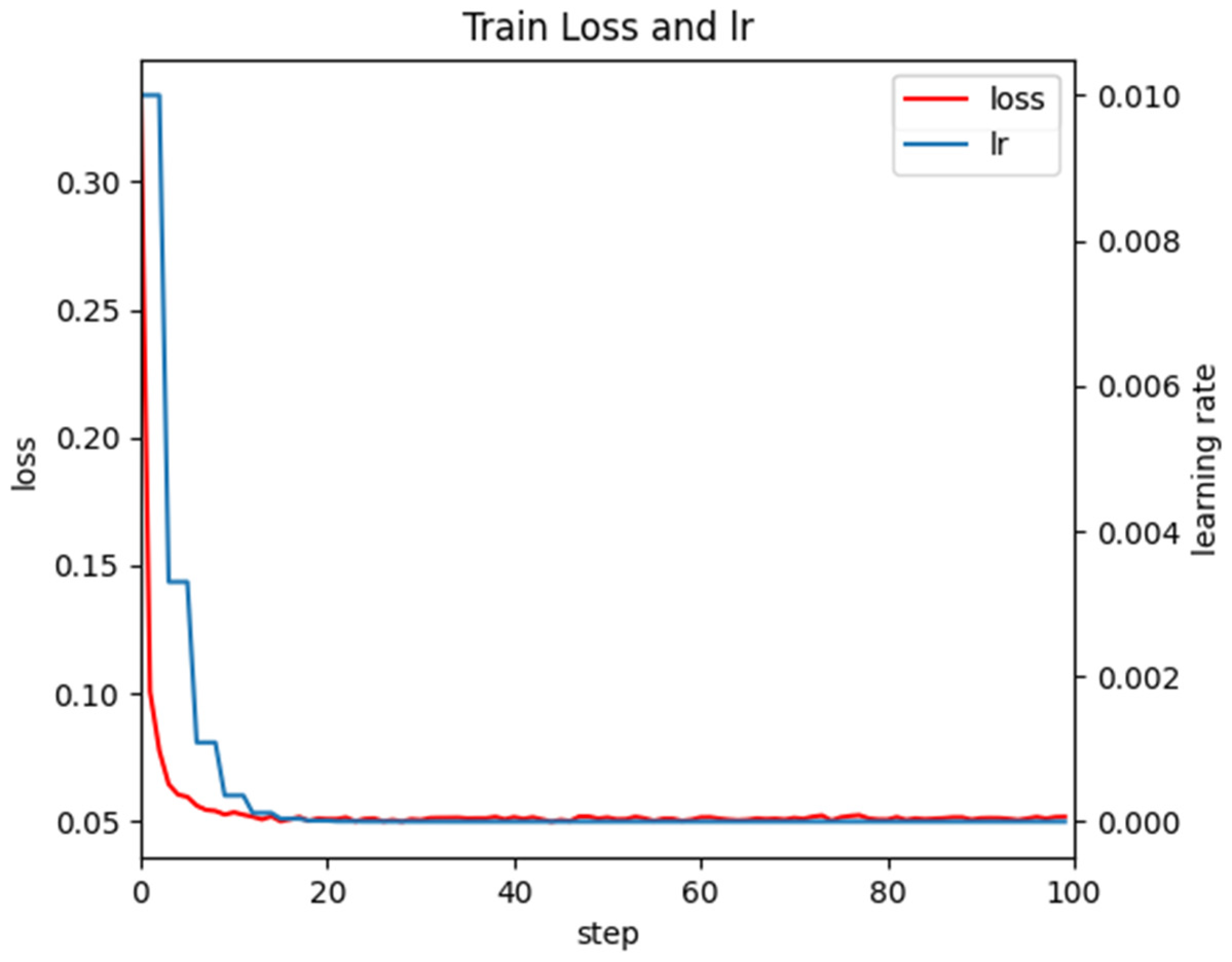
The total loss function and learning rate changes during model training are shown in
Figure 13.
In
Figure 13, the loss value curve, indicated by the red line, is observed to be decreasing in tandem with the learning rate curve, depicted by the blue line, as the number of iterations of FRCNN-PGR is augmented. The decreasing trend of both parameters is sustained until they eventually stabilize.
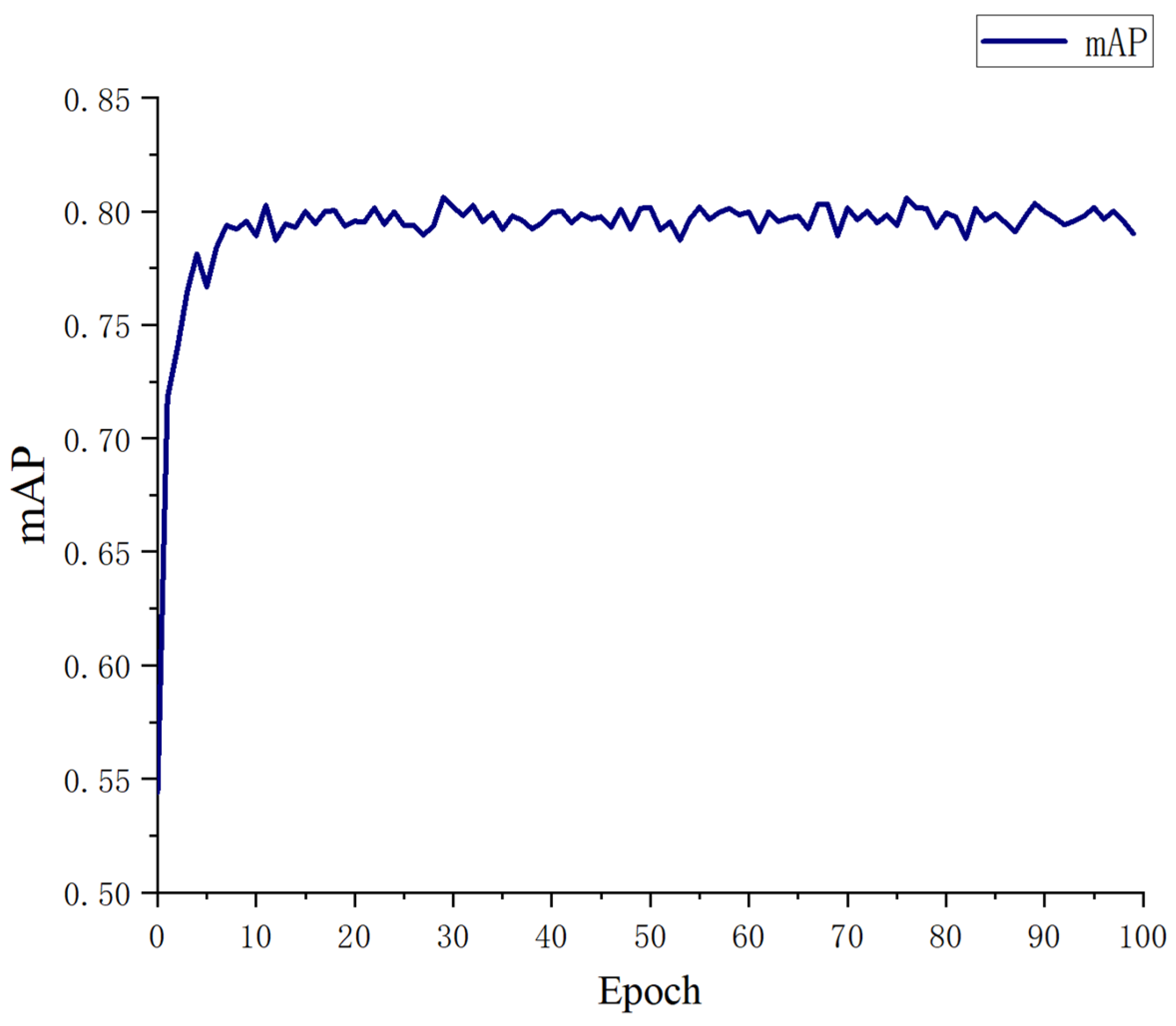
Figure 14 illustrates the changes in mAP during model training, wherein a gradual increase in mAP is observed with the continuation of training iterations until it ultimately reaches a stable state.
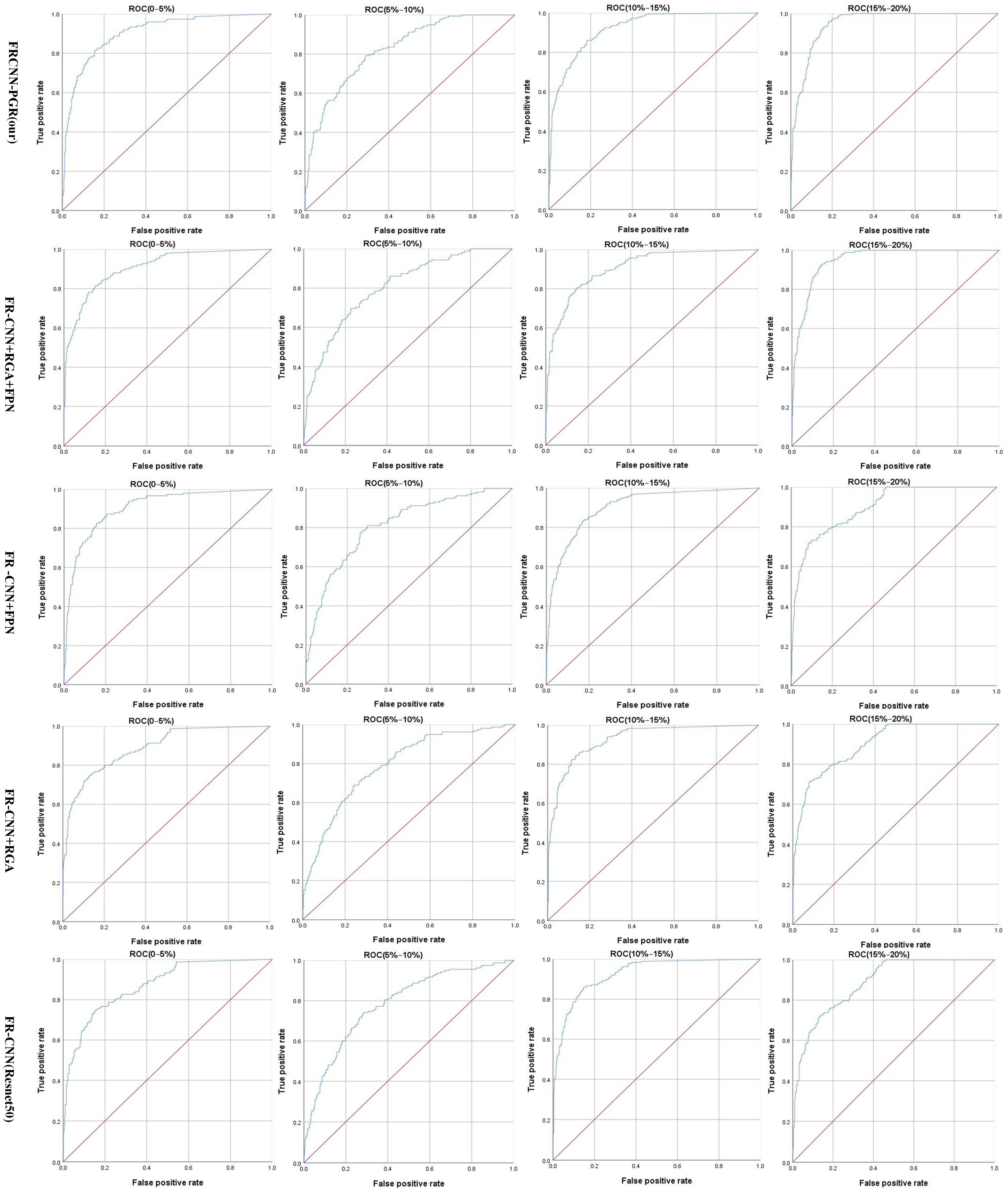
The ROC curves of different models in each grade category are shown in
Figure 15.
The Receiver Operating Characteristic (ROC) curve is a graphical representation that elucidates the interdependence between sensitivity and specificity in a given classification model. Upon meticulous scrutiny of
Figure 15, it is evident that the model in question has undergone a series of enhancements, resulting in a gradual amplification in the Area Under Curve (AUC) value. This surge in the AUC value unequivocally signifies that the predictive performance of our model has been consistently ameliorated over time.
The comparison between the different models (FR-CNN, FR-CNN + RGA, FR-CNN + FPN, FR-CNN + RGA + FPN, and FRCNN-PGR) and the experimental results are shown in
Table 3, and the FPR and FNR of each model in different graphite ore grade categories are shown in
Table 4.
The comparative data displayed in
Table 3 evinces a discernible augmentation in the precision and recall rates of the primary model of the faster R-CNN algorithm for the recognition of graphite mine images, as a direct consequence of employing the FRCNN-PGR algorithm. The data further suggest that the mean average precision (mAP) has increased by 5.3%, whilst the recall rate has surged by 1.9%. Moreover, upon scrutinizing the false positive rate (FPR) and false negative rate (FNR) values, alongside the macro-average values of both the native and FRCNN-PGR models, as presented in
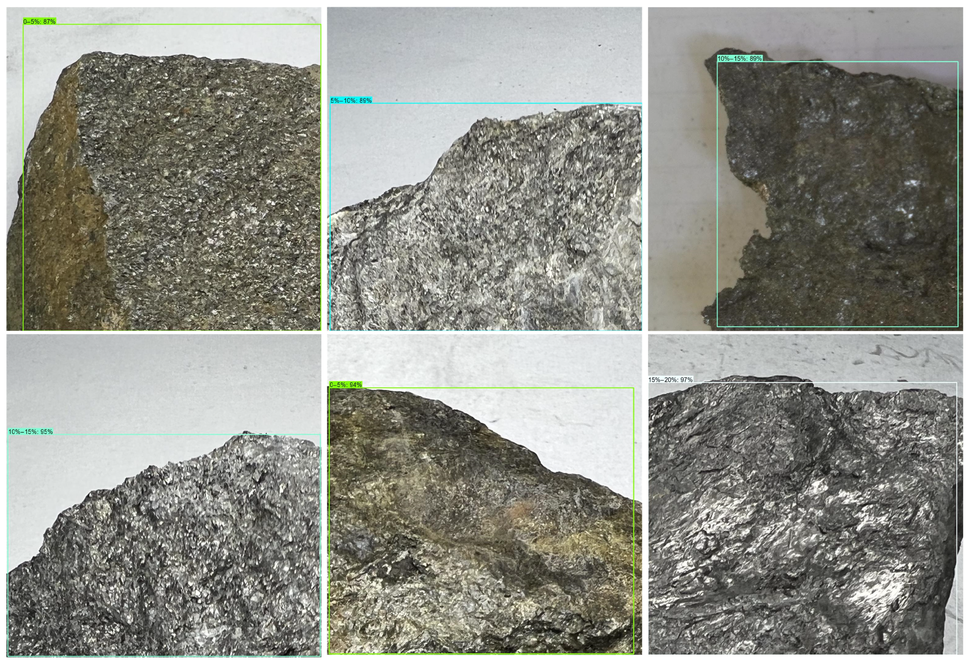
Table 4, it can be inferred that our proposed model yields superior performance, overall. Furthermore, the macro-average value exhibits a progressive decrease, which further substantiates our model’s enhanced performance. Finally,
Figure 16 illustrates the outcomes of the graphite mine image recognition, based on the FRCNN-PGR model.
5. Conclusions
This paper proposes a novel solution to the complexity of traditional graphite ore grade detection by introducing a more convenient and concise FRCNN-PGR model method. The traditional method is plagued by a high level of complexity, which makes it impractical for real-world applications. The proposed method involves cutting the original graphite ore image during data processing to obtain a larger number of training images that provide a better texture detail recognition effect. Moreover, a bottom–up feature extraction is executed on the underlying feature maps to generate a series of feature maps with different scales, which are then fused through a top–down feature fusion to obtain a pyramid structure of feature maps. To improve the Faster R-CNN model, the global attention mechanism RGA is introduced to accurately grasp the entire image from spatial and channel levels. Additionally, the FRN layer replaces the BN layer, while the activation function ReLU becomes the TLU function, which enhances the small batch model’s training performance. The FRCNN-PGR algorithm shows better performance and stronger robustness, enabling it to identify the image grade of graphite ore within a smaller margin of error. While the detection time is slightly increased compared to the original model, the improved model demonstrates enhanced recognition accuracy within different grade ranges and greater robustness, substantially reducing the workload of pre-detecting graphite ore grade. Future experiments will further explore the model’s recognition performance under different lighting conditions, such as night and rain, ultimately enhancing its stability in any real-world scenario.


