


Numerical Performance of a Buoy-Type Wave Energy Converter with Regular Short Waves


Abstract
1. Introduction
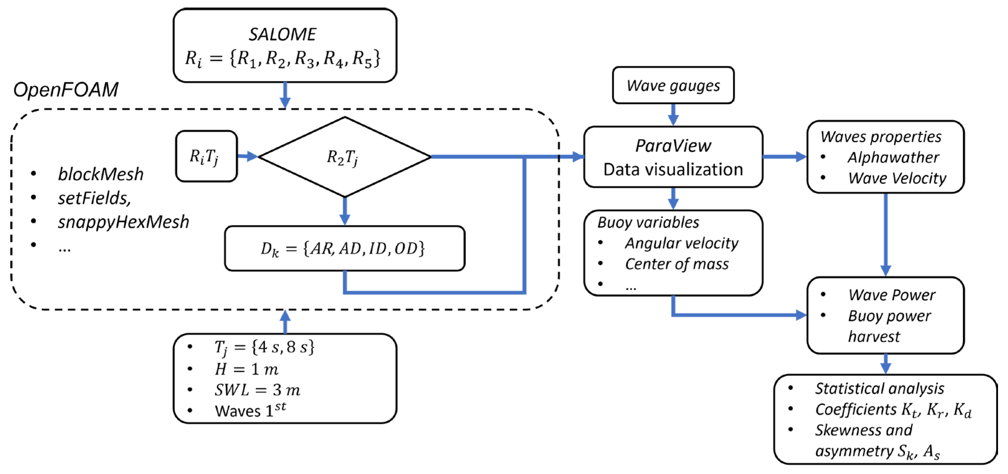
2. Simulation Framework
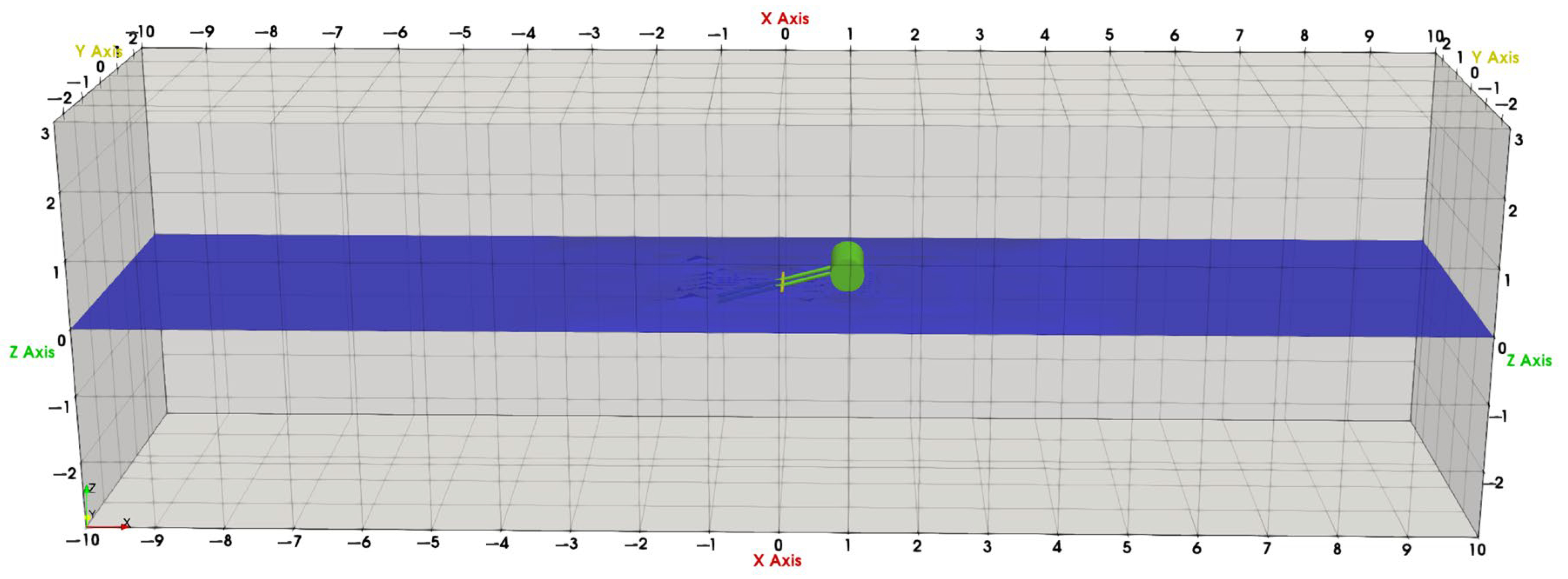
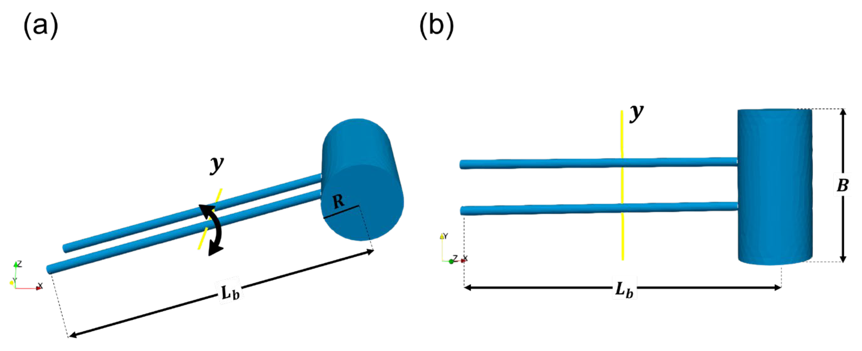
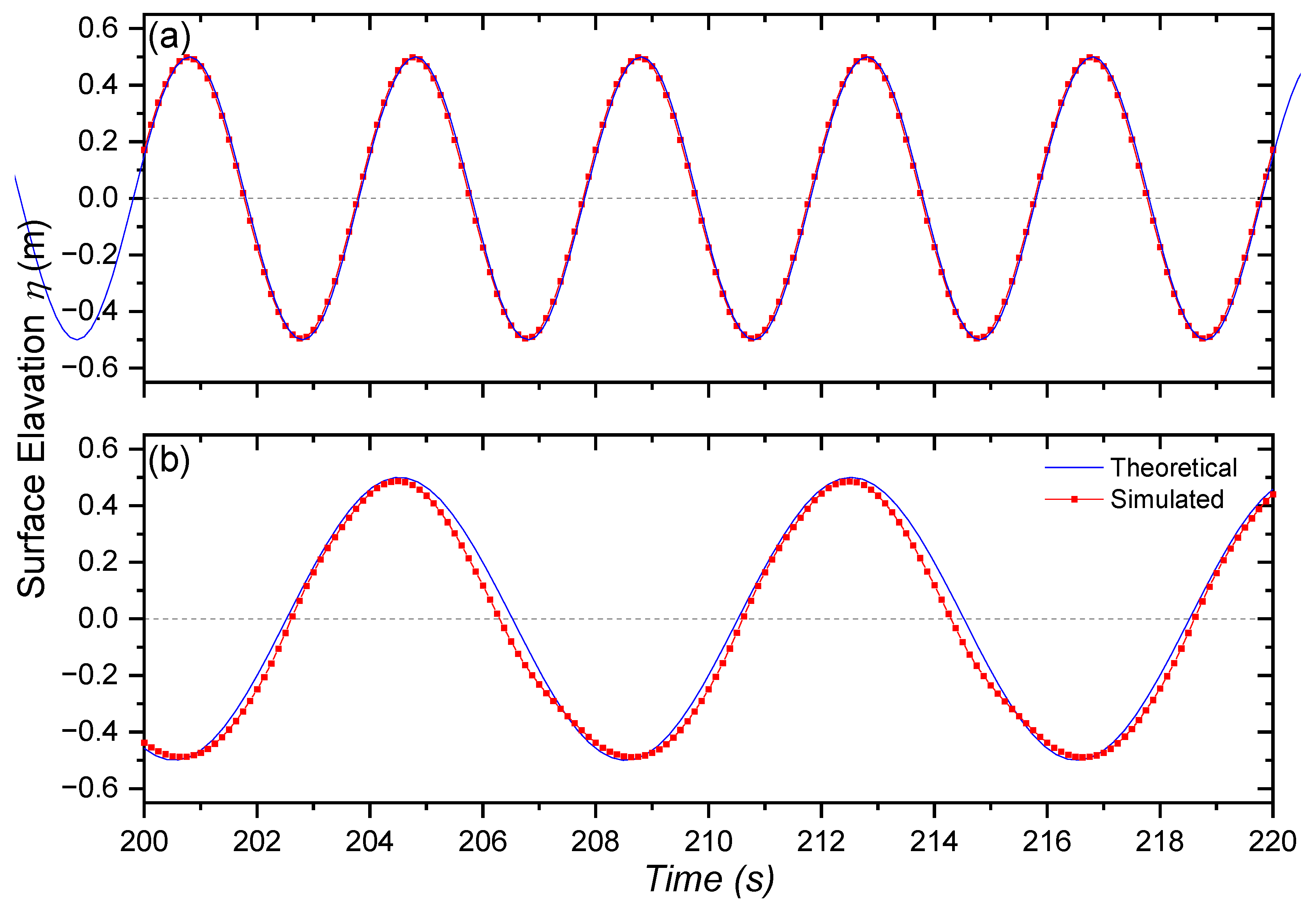
2.1. Numerical Model
2.2. Simulation Setup
3. Calculations of Wave Power
3.1. Wave Power and Its Absorption by the Buoy
3.2. Bulk Parameters and Nonlinear Wave Properties
4. Results and Discussion
4.1. Execution Time and Model Stability
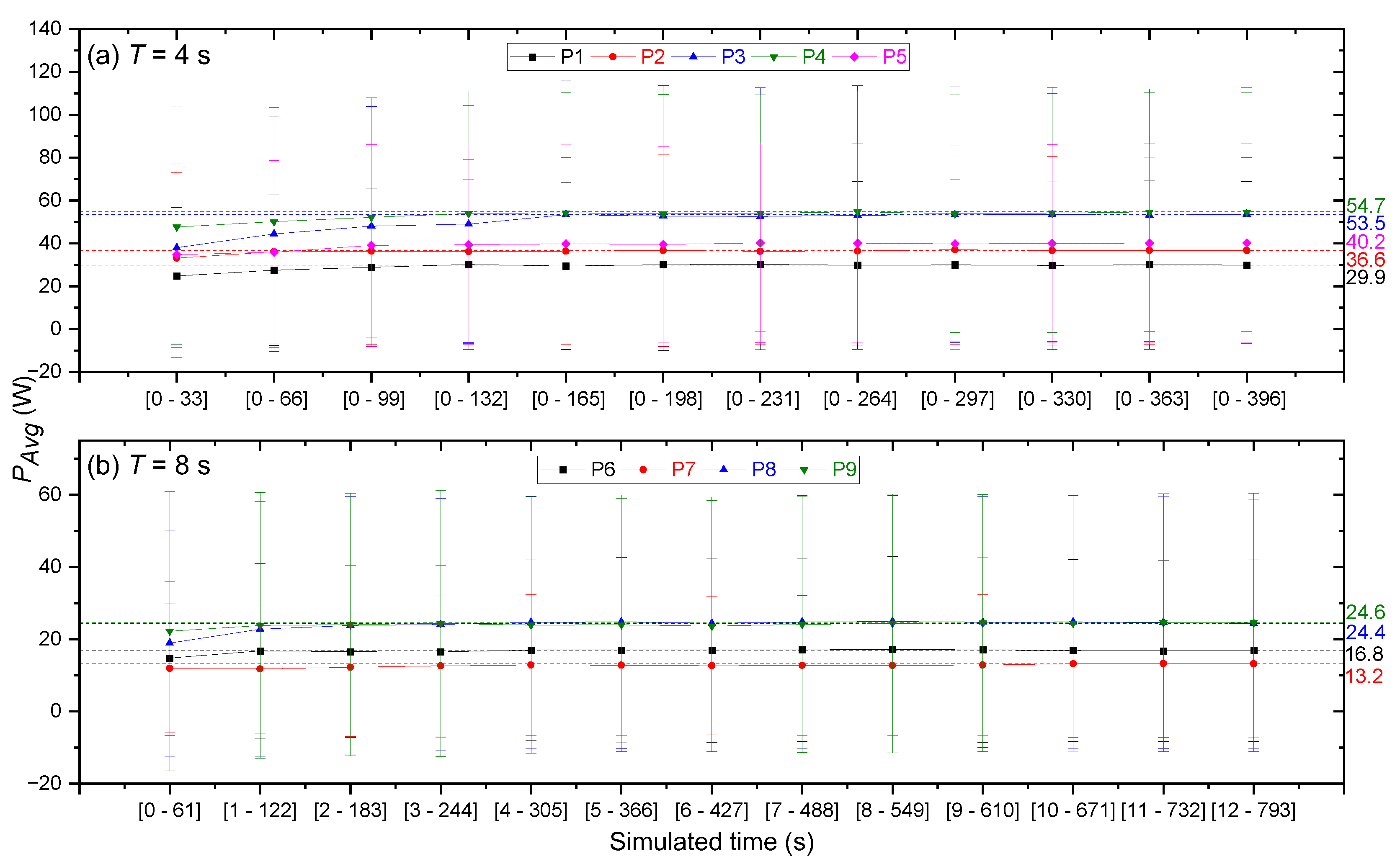
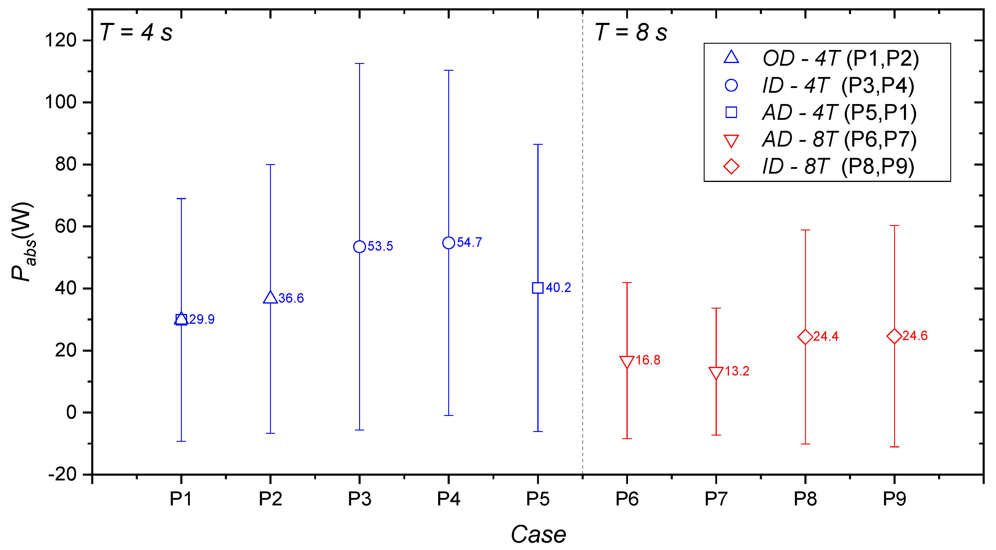
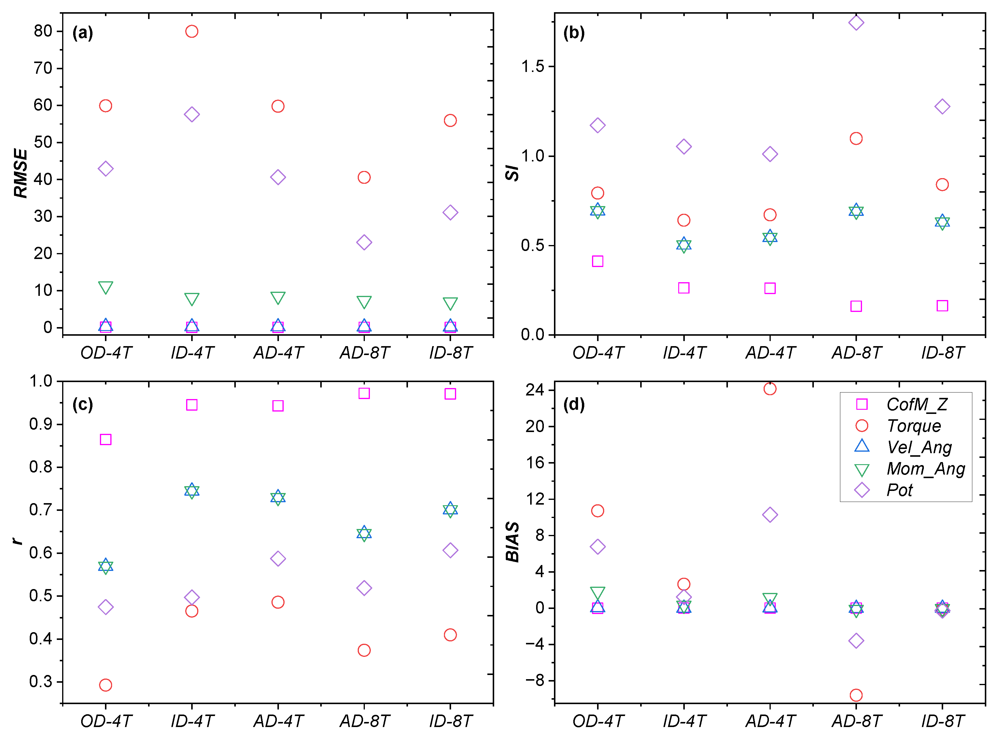
4.2. Sensitivity Tests
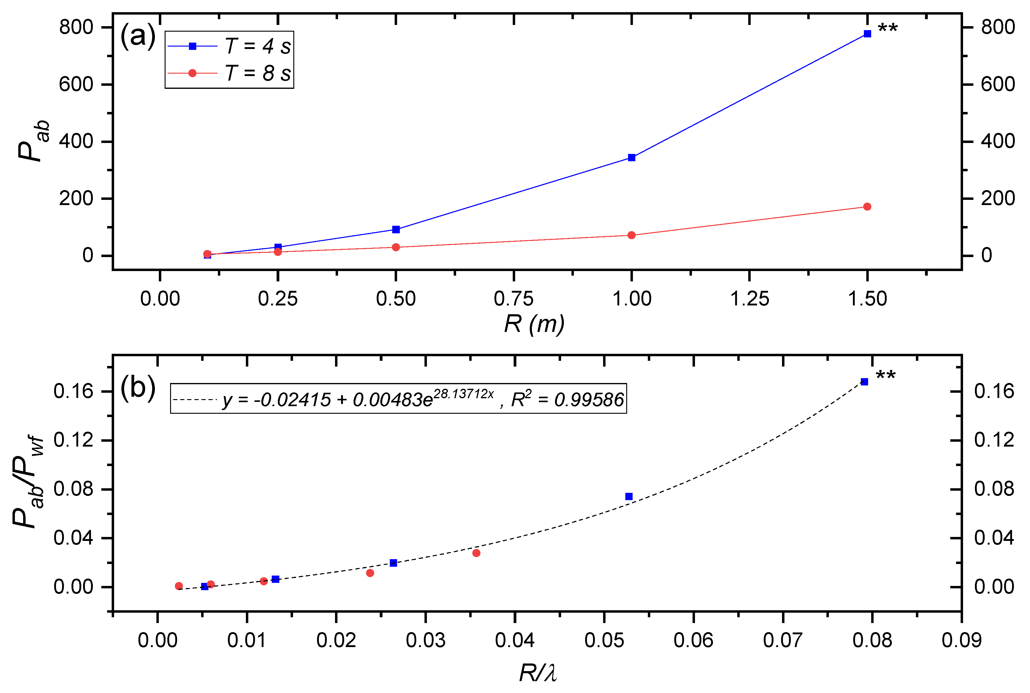
4.3. WEC Power Absorption
4.4. Potential Effects of the WEC on Sediment Transport and Coastal Protection
5. Conclusions and Recommendations
5.1. Conclusions
5.2. Recommendations
Author Contributions
Funding
Data Availability Statement
Conflicts of Interest
References
- Gunn, K.; Stock-Williams, C. Quantifying the global wave power source. Renew. Energy 2012, 44, 296–304. [Google Scholar] [CrossRef]
- Polinder, H.; Scuotto, M. Wave energy converters and their impact on power systems. In Proceedings of the 2005 International Conference on Future Power Systems, Amsterdam, The Netherlands, 18 November 2005; Available online: https://ieeexplore.ieee.org/document/1600483 (accessed on 27 March 2023).
- Henriques, J.C.C.; Gato, L.M.C.; Falcao, A.F.O.; Robles, E.; Fay, F.X. Latching control of a floating oscillating-water-column wave energy converter. Renew. Energy 2016, 90, 229–241. [Google Scholar] [CrossRef]
- Esmaeilzadeh, S.; Alam, M.R. Shape optimization of wave energy converters for broadband directional incident waves. Ocean Eng. 2019, 174, 186–200. [Google Scholar] [CrossRef]
- Garcia-Teruel, A.; Forehand, D.I.M. A review of geometry optimisation of wave energy converters. Renew. Sustain. Energy Rev. 2021, 139, 110593. [Google Scholar] [CrossRef]
- Trapani, K.; Millar, D.L.; Smith, H.C.M. Novel offshore application of photovoltaics in comparison to conventional marine renewable energy technologies. Renew. Energy 2013, 50, 879–888. [Google Scholar] [CrossRef]
- Dalton, G.J.; Alcorn, R.; Lewis, T. Case study feasibility analysis of the Pelamis wave energy convertor in Ireland, Portugal and North America. Renew. Energy 2010, 35, 443–455. [Google Scholar] [CrossRef]
- The European Marine Energy Centre LTD. Press Release: Council Takes Ownership of Pelamis Device, 6 July 2017. Available online: http://www.emec.org.uk/press-release-council-takes-ownership-of-pelamis-device/ (accessed on 27 March 2023).
- The European Marine Energy Centre LTD. Aquamarine Power. Available online: http://www.emec.org.uk/about-us/wave-clients/aquamarine-power/ (accessed on 27 March 2023).
- Carnegie Clean Energy. CETO 5-Perth (WA). Available online: https://www.carnegiece.com/portfolio/ceto-5-perth-wa/ (accessed on 27 March 2023).
- Hoefel, F.; Elgar, S. Wave-Induced Sediment Transport and Sandbar Migration. Science 2003, 299, 1885–1887. [Google Scholar] [CrossRef]
- Astariz, S.; Iglesias, G. The economics of wave energy: A review. Renew. Sustain. Energy Rev. 2015, 45, 397–408. [Google Scholar] [CrossRef]
- Teixeira-Duarte, F.; Clemente, D.; Gianini, G.; Rosa-Santos, P.; Taveira-Pinto, F. Review on layout optimization strategies of offshore parks for wave energy converters. Renew. Sustain. Energy Rev. 2022, 163, 112513. [Google Scholar] [CrossRef]
- Karan, H.; Thomson, R.C.; Harrison, G.P. Full life cycle assessment of two surge wave energy converters. Proc. IMechE Part A J. Power Energy 2020, 234, 548–561. [Google Scholar] [CrossRef]
- Nasrollahi, S.; Kazemi, A.; Jahangir, M.-H.; Aryaee, S. Selecting suitable wave energy technology for sustainable development, an MCDM approach. Renew. Energy 2023, 202, 756–772. [Google Scholar] [CrossRef]
- Foteinis, S. Wave energy converters in low energy seas: Current state and opportunities. Renew. Sustain. Energy Rev. 2022, 162, 112448. [Google Scholar] [CrossRef]
- Xu, R.; Wang, H.; Xi, Z.; Wang, W.; Xu, M. Recent progress on wave energy marine buoys. J. Mar. Sci. Eng. 2022, 10, 566. [Google Scholar] [CrossRef]
- Falnes, J.; Kurniawan, A. Ocean Waves and Oscillating Systems: Linear Interactions Including Wave-Energy Extraction; Cambridge University Press: Cambridge, UK, 2020; Volume 8. [Google Scholar]
- Greenshields, C.J. OpenFOAM User Guide Version 5.0; The OpenFOAM Foundation: London, UK, 2015; p. 47. [Google Scholar]
- Windt, C.; Davidson, J.; Ringwood, J.V. High-fidelity numerical modelling of ocean wave energy systems: A review of computational fluid dynamics-based numerical wave tanks. Renew. Sustain. Energy Rev. 2018, 93, 610–630. [Google Scholar] [CrossRef]
- Giorgi, G.; Penalba Retes, M.; Ringwood, J.V. Nonlinear Hydrodynamic Models for Heaving Buoy Wave Energy Converters. In Proceedings of the 3rd Asian Wave and Tidal Energy Conference, Singapore, 2016; Available online: https://tethys-engineering.pnnl.gov/publications/nonlinear-hydrodynamic-models-heaving-buoy-wave-energy-converters (accessed on 27 March 2023).
- Windt, C.; Davidson, J.; Akram, B.; Ringwood, J.V. Performance assessment of the overset grid method for numerical wave tank experiments in the OpenFOAM environment. In Proceedings of the 37th International Conference on Ocean, Offshore and Arctic Engineering, Madrid, Spain, 17–22 June 2018; American Society of Mechanical Engineers: Madrid, Spain, 2018. [Google Scholar]
- Davidson, J.; Karimov, M.; Szelechman, A.; Windt, A.; Ringwood, J. Dynamic mesh motion in OpenFOAM for wave energy converter simulation. In Proceedings of the 14th OpenFOAM Workshop, Duisburg, Germany, 23–26 July 2019. [Google Scholar] [CrossRef]
- Windt, C.; Davidson, J.; Chandar, D.D.J.; Faedo, N.; Ringwood, J.V. Evaluation of the overset grid method for control studies of wave energy converters in OpenFOAM numerical wave tanks. J. Ocean Eng. Mar. Energy 2020, 6, 55–70. [Google Scholar] [CrossRef]
- Windt, C.; Davidson, J.; Chandar, D.; Ringwood, J.V. On the importance of advanced mesh motion methods for WEC experiments in CFD-based numerical wave tanks. In Proceedings of the VIII International Conference on Computational Methods in Marine Engineering, CIMNE, Gothenburg, Sweden, 13–15 May 2019; pp. 145–156. Available online: https://www.semanticscholar.org/paper/On-the-Importance-of-Advanced-Mesh-Motion-Models-in-Windt-Davidson/4db8059cbaa4e7a2ac56bfaf9df16da4f3e339e6 (accessed on 27 March 2023).
- OpenFOAM. 6.2 Numerical Schemes. Available online: https://www.openfoam.com/documentation/user-guide/6-solving/6.2-numerical-schemes (accessed on 29 March 2023).
- Devolder, B.; Schmitt, P.; Rauwoens, P.; Elsaesser, B.; Troch, P. A review of the implicit motion solver algorithm in OpenFOAM® to simulate a heaving buoy. In Proceedings of the 18th Numerical Towing Tank Symposium, Cortona, Italy, 2015; Available online: https://www.semanticscholar.org/paper/A-Review-of-the-Implicit-Motion-Solver-Algorithm-in-Devolder-Schmitt/cf5ec01ae9176fe20a4a732840e320c5a58e08cc (accessed on 27 March 2023).
- Holzmann, T. Mathematics, numerics, derivations and OpenFOAM®. In The Basics for Numerical Simulations; Holzman CFD: Loeben, Germany, 2016. [Google Scholar]
- Chow, J.H.; Ng, E.Y.K. Strongly coupled partitioned six degree-of-freedom rigid body motion solver with Aitken’s dynamic under-relaxation. Int. J. Nav. Archit. Ocean. Eng. 2016, 8, 320–329. [Google Scholar] [CrossRef]
- SALOME, The Open Source Integration Platform for Numerical Simulation. Available online: https://www.salome-platform.org/ (accessed on 29 March 2023).
- Jacobsen, N.G. waves2Foam Manual; Deltares: Delft, The Netherlands, 2017. [Google Scholar]
- Dhanak, M.R.; Xiros, N.I. (Eds.) Springer Handbook of Ocean Engineering; Springer: Berlin/Heidelberg, Germany, 2016. [Google Scholar]
- Budar, K.; Falnes, J. A resonant point absorber of ocean-wave power. Nature 1975, 256, 478–479. [Google Scholar] [CrossRef]
- Evans, D.V. A theory for wave-power absorption by oscillating bodies. J. Fluid Mech. 1976, 77, 1–25. [Google Scholar] [CrossRef]
- Falcao, A. Wave energy utilization: A review of the technologies. Renew. Sustain. Energy Rev. 2010, 14, 899–918. [Google Scholar] [CrossRef]
- Babarit, A. Ocean Wave Energy Conversion: Resource, Technologies and Performance; Elsevier: Amsterdam, The Netherlands, 2017. [Google Scholar]
- Babarit, A. A database of capture width ratio of wave energy converters. Renew. Energy 2015, 80, 610–628. [Google Scholar] [CrossRef]
- Abanades, J.; Greaves, D.; Iglesias, G. Wave farm impact on the beach profile: A case study. Coast. Eng. 2014, 86, 36–44. [Google Scholar] [CrossRef]
- Loukili, M.; Dutykh, D.; Pincemin, S.; Kotrasova, K.; Abcha, N. Theoretical Investigation Applied to Scattering Water Waves by Rectangular Submerged Obstacles/and Submarine Trenches. Geosciences 2022, 12, 379. [Google Scholar] [CrossRef]
- Seelig, W.N.; Ahrens, J.P. Estimation of Wave Reflection and Energy Dissipation Coefficients for Beaches, Revetments, and Breakwaters; Coastal Engineering Research Center: Fort Belvoir, Virginia, 1981. [Google Scholar]
- Mansard, E.P.D.; Funke, E.R. The measurement of incident and reflected spectra using a least squares method. In Proceedings of the 17th International Conference on Coastal Engineering, Sydney, Australia, 23–28 March 1980; pp. 154–172. Available online: https://repository.tudelft.nl/islandora/object/uuid%3A840a64af-b113-4372-8f91-47b4d7a3cc78 (accessed on 27 March 2023).
- Atan, R.; Finnegan, W.; Nash, S.; Goggins, J. The effect of arrays of wave energy converters on the nearshore wave climate. Ocean Eng. 2019, 172, 373–384. [Google Scholar] [CrossRef]
- Fernández-Mora, A.; Calvete, D.; Falqués, A.; de Swart, H.E. Onshore sandbar migration in the surf zone: New insights into the wave-induced sediment transport mechanisms. Geophys. Res. Lett. 2015, 42, 2869–2877. [Google Scholar] [CrossRef]
- Berni, C.; Barthélemy, E.; Michallet, H. Surf zone cross-shore boundary layer velocity asymmetry and skewness: An experimental study on a mobile bed. J. Geophys. Res. Oceans 2013, 118, 2188–2200. [Google Scholar] [CrossRef]
- Gao, J.-L.; Lyu, J.; Zhang, J.; Liu, Q.; Zang, J.; Zou, T. Study on Transient Gap Resonance with Consideration of the Motion of Floating Body. China Ocean Eng. 2022, 36, 994–1006. [Google Scholar] [CrossRef]
- Gao, J.; He, Z.; Huang, X.; Liu, Q.; Zang, J.; Wang, G. Effects of free heave motion on wave resonance inside a narrow gap between two boxes under wave actions. Ocean Eng. 2021, 224, 108753. [Google Scholar] [CrossRef]
- Qu, S.; Liu, S.; Ong, M.C.; Wang, X.; Sun, S. Numerical simulation of free-surface waves past semi-submerged two-dimensional rectangular prisms with different aspect ratios and rounding chamfer radii. Ocean Eng. 2023, 269, 113604. [Google Scholar] [CrossRef]
- Wang, K.; Ma, X.; Bai, W.; Lin, Z.; Li, Y. Numerical simulation of water entry of a symmetric/asymmetric wedge into waves using OpenFOAM. Ocean Eng. 2021, 227, 108923. [Google Scholar] [CrossRef]
- Palm, J.; Eskilsson, C.; Moura Paredes, G.; Bergdahl, L. Coupled mooring analysis for floating wave energy converters using CFD: Formulation and validation. Int. J. Marine Energy 2016, 16, 83–99. [Google Scholar] [CrossRef]
- Loh, T.T.; Pizer, D.; Simmonds, D.; Kyte, A.; Greaves, D. Simulation and analysis of wave-structure interactions for a semi-immersed horizontal cylinder. Ocean Eng. 2018, 147, 676–689. [Google Scholar]
- Diaz-Maya, M.; Ulloa, M.; Silva, R. Assessing wave energy converters in the gulf of Mexico using a multi-criteria approach. Front. Energy Res. 2022, 10, 929625. [Google Scholar] [CrossRef]
- Dai, J.; Wang, C.M.; Utsunomiya, Y.; Duan, W. Review of recent research and developments on floating breakwaters. Ocean Eng. 2018, 158, 132–151. [Google Scholar] [CrossRef]
- Hu, Z.Z.; Greaves, D.; Raby, A. Numerical wave tank study of extreme waves and wave-structure interaction using OpenFoam®. Ocean Eng. 2016, 126, 329–342. [Google Scholar] [CrossRef]
- Elgar, S.; Guza, R.T.; Freilich, M.H. Eulerian measurements of horizontal accelerations in shoaling gravity waves. J. Geophys. Res. Oceans 1988, 93, 9261–9269. [Google Scholar] [CrossRef]
- Al Shami, E.; Zhang, R.; Wang, X. Point absorber wave energy harvesters: A review of recent developments. Energies 2018, 12, 47. [Google Scholar] [CrossRef]
- Loukili, M.; Dutykh, D.; Hadjib, C.; Ning, D.; Kotrasova, K. Analytical and Numerical Investigations Applied to Study the Reflections and Transmissions of a Rectangular Breakwater Placed at the Bottom of a Wave Tank. Geosciences 2021, 11, 430. [Google Scholar] [CrossRef]
- Ozkop, E.; Altas, I.H. Control, power and electrical components in wave energy conversion systems: A review of the technologies. Renew. Sustain. Energy Rev. 2017, 67, 106–115. [Google Scholar] [CrossRef]


| Units | Water | Air | |
|---|---|---|---|
| Kinematic viscosity | |||
| Density | .0 | 1.0 | |
| Surface tension between the two phases | |||
| Buoy | |||
|---|---|---|---|
| R1 | 0.10 | 1.5 | 0.067 |
| R2 | 0.25 | 2.0 | 0.125 |
| R3 | 0.50 | 3.0 | 0.167 |
| R4 | 1.00 | 4.0 | 0.250 |
| R5 | 1.50 | 6.0 | 0.250 |
| T = 4 s | T = 8 s | |
|---|---|---|
| Computation Time (Hours) | ||
| 127.23 | 260.23 | |
| 226.01 | 491.94 | |
| 615.93 | 1246.81 | |
| 1196.84 | 2390.67 | |
| 2027.45 | 3488.00 | |
| Case | T (s) | AR | AD | ID | OD |
|---|---|---|---|---|---|
| P1 | 4 | 0.7 | 1.0 | 0.001 | 1.5 |
| P2 | 0.7 | 1.0 | 0.001 | 2.0 | |
| P3 | 0.5 | 0.5 | 0.001 | 1.5 | |
| P4 | 0.5 | 0.5 | 0.00001 | 1.5 | |
| P5 | 0.7 | 0.75 | 0.001 | 1.5 | |
| P6 | 8 | 0.7 | 0.75 | 0.001 | 1.5 |
| P7 | 0.7 | 1.0 | 0.001 | 1.5 | |
| P8 | 0.5 | 0.5 | 0.001 | 1.5 | |
| P9 | 0.5 | 0.5 | 0.00001 | 1.5 |
| Test Number | Sensitivity Test | Cases Compared |
|---|---|---|
| 1 | OD-4T | P1, P2 |
| 2 | ID-4T | P3, P4 |
| 3 | AD-4T | P1, P5 |
| 4 | AD-8T | P6, P7 |
| 5 | ID-8T | P8, P9 |
| Buoy | T = 4 s | T = 8 s | ||||
|---|---|---|---|---|---|---|
| 0.298 | 0.005 | 0.698 | 0.477 | 0.006 | 0.517 | |
| 0.300 | 0.004 | 0.695 | 0.489 | 0.006 | 0.506 | |
| 0.298 | 0.005 | 0.698 | 0.484 | 0.005 | 0.511 | |
| 0.290 | 0.006 | 0.704 | 0.480 | 0.005 | 0.515 | |
| 0.284 | 0.013 | 0.704 | 0.474 | 0.007 | 0.519 | |
Disclaimer/Publisher’s Note: The statements, opinions and data contained in all publications are solely those of the individual author(s) and contributor(s) and not of MDPI and/or the editor(s). MDPI and/or the editor(s) disclaim responsibility for any injury to people or property resulting from any ideas, methods, instructions or products referred to in the content. |
© 2023 by the authors. Licensee MDPI, Basel, Switzerland. This article is an open access article distributed under the terms and conditions of the Creative Commons Attribution (CC BY) license (https://creativecommons.org/licenses/by/4.0/).
Share and Cite
Sosa, C.; Mariño-Tapia, I.; Silva, R.; Patiño, R. Numerical Performance of a Buoy-Type Wave Energy Converter with Regular Short Waves. Appl. Sci. 2023, 13, 5182. https://doi.org/10.3390/app13085182
Sosa C, Mariño-Tapia I, Silva R, Patiño R. Numerical Performance of a Buoy-Type Wave Energy Converter with Regular Short Waves. Applied Sciences. 2023; 13(8):5182. https://doi.org/10.3390/app13085182
Chicago/Turabian StyleSosa, Carlos, Ismael Mariño-Tapia, Rodolfo Silva, and Rodrigo Patiño. 2023. "Numerical Performance of a Buoy-Type Wave Energy Converter with Regular Short Waves" Applied Sciences 13, no. 8: 5182. https://doi.org/10.3390/app13085182
APA StyleSosa, C., Mariño-Tapia, I., Silva, R., & Patiño, R. (2023). Numerical Performance of a Buoy-Type Wave Energy Converter with Regular Short Waves. Applied Sciences, 13(8), 5182. https://doi.org/10.3390/app13085182