A Transfer Residual Neural Network Based on ResNet-50 for Detection of Steel Surface Defects

Abstract

With the increasing popularity of deep learning, enterprises are replacing traditional inefficient and non-robust defect detection methods with intelligent recognition technology. This paper utilizes TL (transfer learning) to enhance the model’s recognition performance by integrating the Adam optimizer and a learning rate decay strategy. By comparing the TL-ResNet50 model with other classic CNN models (ResNet50, VGG19, and AlexNet), the superiority of the model used in this paper was fully demonstrated. To address the current lack of understanding regarding the internal mechanisms of CNN models, we employed an interpretable algorithm to analyze pre-trained models and visualize the learned semantic features of defects across various models. This further confirms the efficacy and reliability of CNN models in accurately recognizing different types of defects. Results showed that the TL-ResNet50 model achieved an overall accuracy of 99.4% on the testing set and demonstrated good identification ability for defect features.

1. Introduction

As a crucial product in the steel industry, flat steel has a wide application in industries such as shipbuilding, aviation, manufacturing, and automobiles. It constitutes more than 65% of the steel production capacity. Therefore, any quality issues with steel can result in significant losses for manufacturers and consumers alike. Notably, the biggest threat to thin and wide flat steel is surface defects [1].

Due to low efficiency and high subjectivity, traditional manual detection methods are being steadily replaced by various detection algorithms. However, poor robustness and real-time performance make it difficult for some defect detection algorithms, such as edge detection [2], wavelet transform [3], genetic algorithm [4], support vector machine [5], and so on, to meet the requirements of online defect detection. As a result, the intelligent development of steel defect detection is greatly limited. With the ongoing development of deep learning technology, an increasing number of companies are introducing intelligent recognition technology to replace traditional defect detection algorithms [6]. The use of convolutional neural networks (CNNs) [7,8] in steel surface defect recognition significantly improves its accuracy. He et al. [9] introduced a multi-level feature fusion network that achieved 92% accuracy by fusing picture characteristics obtained at each stage. Hao et al. [10] proposed the DF-ResNet50 network model, which applies a characteristic neural network and decentralized attention network to enhance steel defect detection performance.

However, achieving relatively reliable accuracy with CNNs requires a large number of training samples, which makes their use difficult for industrial applications. The introduction of TL (transfer learning) has greatly alleviated the problem of model underfitting in small sample settings. By utilizing pre-trained models trained on large-scale datasets [11], TL applies feature extraction capabilities learned from a vast number of samples to other fields [12].

Regarding the application of TL, Wu et al. [13] used a TL model to improve steel defect detection and experimentally verified that this approach outperforms traditional CNNs in terms of both training and testing accuracy, achieving an accuracy of approximately 98%. Based on these findings, Bouguettaya et al. [14] studied the effectiveness of combining two CNN architectures (MobileNet-V2 and Xception) with TL, proposing a method that not only achieves high recognition accuracy but also quickly executes. Wan et al. [15] improved the VGG19 network based on fast image preprocessing algorithms and TL, resulting in a recognition accuracy of 97.8% even under conditions of few samples and imbalanced datasets.

It can be seen from the above that using TL-based CNN models can enhance defect detection performance. However, due to their numerous parameters, CNNs can display unpredictable behavior [16]. For example, even if CNN has superior performance and good generalization on object recognition tasks, Szegedy et al. [17] found a method to arbitrarily alter the network’s prediction results by making imperceptible changes to input images. These modified inputs are called “adversarial examples”. Nguyen et al. [18] showed a method to generate images that are similar to white noise, and which are very difficult for humans to recognize. However, CNNs can identify them as objects with very high confidence (99.99%). The above research indicates that while CNNs perform well on many tasks, their underlying mechanisms may significantly differ from those of humans and are not yet fully comprehended. There is still a lack of explanatory analysis in steel surface defect recognition applications.

This paper attempts to apply an interpretable algorithm to perform explanatory analysis on pre-trained models in order to reveal why the model has good recognition performance and to explore its focus on different types of defects. The necessity of explanatory analysis has been emphasized in papers [19,20,21]. Therefore, conducting explanatory analysis on steel surface defects is of great significance. It should be noted that interpretable analysis does not make the model more reliable or perform better, but it is an important component in developing more reliable recognition models.

In our study, we compared the performance of three CNN models for steel surface defect recognition: TL-ResNet50, VGG19, and AlexNet. AlexNet [22] was the first CNN model for large-scale image classification problems, featuring five convolutional layers and three fully connected layers. VGG19 [23] has 19 convolutional layers and three fully connected layers, utilizing smaller kernel sizes and repeated convolutional layers to achieve a deeper network structure. TL-ResNet50 [24] is a TL model consisting of 50 layers and special residual blocks. It overcomes the problem of CNN degradation by using residual connections and incorporating multiple residual blocks for greater depth and improved accuracy. Comparing these three models can help highlight TL-ResNet50’s advantages in terms of both convergence speed and accuracy.

In summary, this paper’s primary contributions and innovation points are as follows:

(1)

We utilized TL to load the TL-ResNet50 model and then applied the optimized model to identify steel surface defects, achieving an average accuracy of 99.4% with the combination of adaptive estimation and learning rate convergence.

(2)

We compared TL-ResNet50 with other CNN models, including ResNet50, VGG19, and AlexNet, to validate our model’s performance in recognizing defects using multiple evaluation metrics. Furthermore, we confirmed the superiority of TL by comparing the TL-ResNet50 model with ResNet50, which did not use TL.

(3)

We used an interpretable algorithm to analyze pre-trained models (ResNet50, VGG19, and AlexNet) and understand why they perform well in recognizing different types of defects. We also visualized the focus of various convolutional layers on defect features within TL-ResNet50, which helped us understand the model’s effectiveness and approximate localization of steel surface defects under weak supervision.

2. Materials and Methods

The technical route of this article is shown in Figure 1. First, the defective images are preprocessed and divided into a training set and a verification set at an 8:2 ratio. During training, feature information is extracted using TL-ResNet50 in stages 0 to 4. This model uses convolutional layers, batch normalization layers, and activation functions to gradually extract low- to high-level features of images. After training, the model is switched to evaluation mode and tested on randomly selected defective images. Finally, the TL-ResNet50 model and Grad-CAM++ (Gradient-weighted Class Activation Mapping++) algorithm are used to explain the recognition logic inside the model.

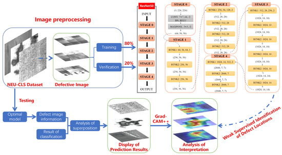
Figure 1. The technical route of this article.

2.1. Dataset

In this study, the experimental samples consisted of common steel surface defect images sourced from the open data provided by Northeastern University, known as the NEU-CLS dataset [25]. The dataset comprised 1800 pieces of 200 × 200-pixel images, with 300 pieces for each of the six types of defects.

The dataset was split into training and testing sets (Table 1) at an 8:2 ratio based on previous experience. Additionally, to make full use of experimental samples, the K-fold cross-validation method was employed during the training phase to analyze the model. This method effectively mitigates overfitting and improves the model’s generalization performance. The training dataset was divided into K-unified sub-datasets, followed by K-model training and verification [26]. During each training cycle, only one sub-dataset was used for verification while the remaining K-1 sub-datasets were used for training. Finally, the average error across K iterations was evaluated.

Table 1. Number of datasets.

Defect Category	Training Set	Test Set
Crazing	240	60
Inclusion	240	60
Patches	240	60
Pitted	240	60
Roll-in scale	240	60
Scratches	240	60
Total	1440	360

Due to the dark color of the steel defect position, identification accuracy suffers when the image background is dark. To address this issue, the transform composition method was employed in this article. Pre-processing the photograph enhanced the contrast between the fault characteristics and the background, making it easier to identify defects. Figure 2 demonstrates some examples of defective images after processing.

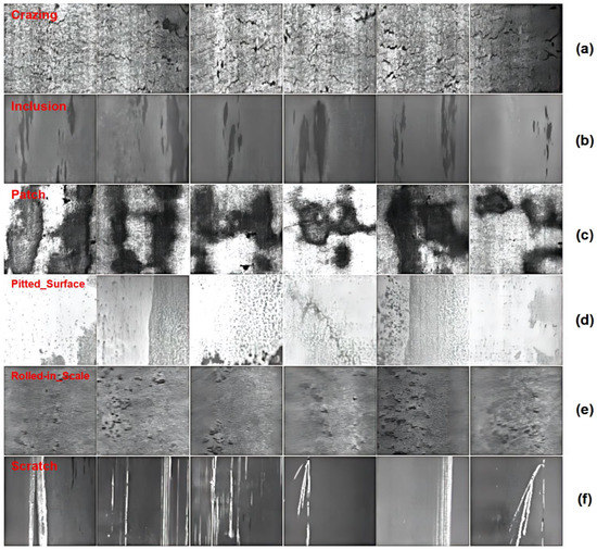
Figure 2. Six common steel surface defects: (a) crazing; (b) inclusion; (c) patches; (d) pitted surface; (e) roll-in scale; (f) scratches.

2.2. ResNet-50 and Transfer Learning

2.2.1. ResNet50

In response to challenges of gradient disappearance/explosion that may occur during training, He. et al. [24] proposed a new residual network called ResNet. This model simplifies network training while addressing the issue of network degradation. Their 152-layer residual network achieved an impressive 3.57% error on the ImageNet dataset.

The classic ResNet50 model is based on the VGG model’s entire 3 × 3 convolutional layer, with each residual block containing two identical 1 × 1 convolution layers. A batch normalization layer and ReLU activation function are connected after each convolutional layer. Lastly, the softmax function is applied for normalization. The ResNet50 network structure is shown in Table 2 [27].

Table 2. The network structure of ResNet50.

Layer Name	Output Size	50-Layer
Conv1	112 × 112	7 × 7,64, stride 2
Conv2.x	56 × 56	3 × 3 max pool, stride 2
		$\left[\begin{array}{cc}1\times 1& 64\\ 3\times 3& 64\\ 1\times 1& 256\end{array}\right]\times 3$
Conv3.x	28 × 28	$\left[\begin{array}{cc}1\times 1& 128\\ 3\times 3& 128\\ 1\times 1& 512\end{array}\right]\times 4$
Conv4.x	14 × 14	$\left[\begin{array}{cc}1\times 1& 256\\ 3\times 3& 256\\ 1\times 1& 1024\end{array}\right]\times 6$
Conv5.x	7 × 7	$\left[\begin{array}{cc}1\times 1& 512\\ 3\times 3& 512\\ 1\times 1& 2048\end{array}\right]\times 3$
	1 × 1	Average pool, 1000-d fc, softmax
FLOPs		3.8 × 109

2.2.2. Transfer Learning

TL involves leveraging knowledge acquired from one or more source tasks to facilitate feature extraction in a target domain, particularly when data samples are limited. In this study, we loaded a TL-ResNet50 model pre-trained on ImageNet data using the PyTorch third-party library, fine-tuning the output feature parameters while keeping the remaining layers frozen. Specifically, the TL-ResNet50 model trained on the ImageNet Large Scale Visual Recognition Challenge (ILSVRC) 2012 dataset, a dataset that contains over one million natural scene images with a size of 224 × 224 pixels. To accommodate the six types of steel defects, the original output feature of the pre-trained TL-ResNet50 model, a 2048-dimensional vector, needs to be modified to 6 dimensions. TL aids in identifying steel surface flaws’ edges, textures, and shapes by extracting more generic features, thus reducing training time.

2.3. An improved CNN Based on ResNet50

2.3.1. ReLU Nonlinear Activation Function

ReLU is the most commonly used activation function in deep learning. It is widely preferred in deep learning because it provides a simple non-linear transformation that can significantly alleviate gradient disappearance issues. The ReLU function can be defined as [28]:

$$ReLU(X)=\max (x,0)$$

(1)

2.3.2. Adaptive Estimation

Traditional random gradients always use a single learning rate (Alpha) to update all weights, which remains constant throughout the training process. While this strategy is efficient, it often requires constantly adjusting the learning rate for the model to optimally converge, leading to time wastage. The Adam algorithm [28], on the other hand, is a self-adaptation estimate that generates independent adaptive learning rates for different parameters. This approach is easy to implement, computationally efficient, and requires minimal memory.

The Adam algorithm builds upon the RMSProp algorithm by using an index-weighted moving average. Its definition is as follows:

$$v_t\leftarrow (1-{\beta }_2){\displaystyle \sum _{\mathrm{i}=1}^{\mathrm{t}}{\beta }_2^{\mathrm{t}-\mathrm{i}}}\cdot g_{\mathrm{i}}^2$$

(2)

In the formula, the super parameter 0 < β₂ < 1 (0.999 is recommended), v_t is the time step momentum, and g_i is the small batch random gradient.

This article utilizes the Adam optimizer in combination with the learning rate decrease method. Specifically, after 10 training cycles, the model’s learning rate is halved. This enables a higher learning rate during the early training phase to accelerate network convergence and a lower learning rate during the late training phase to improve convergence toward optimal solutions. The combination of the Adam algorithm with the learning rate reduction strategy leads to further increased convergence speed and accuracy of the model.

2.3.3. Cross-Entropy Function

The cross-entropy loss function [29] is widely used to increase prediction accuracy by evaluating the differences between the real and predicted probability distributions. This technique solely focuses on the predicted likelihood of an outcome, and as long as its value is significant enough, the prediction result can be considered accurate. By utilizing this strategy, the weight (W) and deviation (B) can be rapidly adjusted, significantly improving the model’s training speed and accuracy. The definition of the cross-entropy loss function is presented below:

$$H(y^{(i)},{\widehat{y}}^{(i)})=-{\displaystyle {\sum }_{j=1}^q{y}_j^{(i)}}\log {\widehat{y}}_j^{(i)}$$

(3)

In the formula, the $y_j^{\left(i\right)}$ vector is an element of the $y^{\left(i\right)}$ vector that is not 0 or 1, and $y^{\left(i\right)}$ is the discrete value of the sample i category.

2.3.4. Network Structure

The TL-ResNet50 model has 50 neural network layers and 5 convolutional kernels, with each layer composed of fundamental convolutional computations (CONV, BN, ReLU). The stage 0 convolutional layer is a straightforward process that involves processing the training set with a single computation. Stages 1 to 4 use a bottleneck structure that consists of multiple identical residual components, with stage 1 introducing residual blocks to solve problems related to gradient disappearance and explosion while improving feature extraction efficiency. Subsequent stages (2/3/4) gradually extract more abstract and advanced features, with stage 4 being the final stage for target classification tasks.

The bottleneck basic residual module (BTNK1 and BTNK2) located on the right side of Figure 3 is a core component of ResNet50. To support deeper networks, He et al. [24] proposed another residual basic block, namely the bottleneck basic residual module, which is utilized in ResNet50 and deeper neural networks. In contrast to the BasicBlock used in shallow networks, the bottleneck block incorporates a 1 × 1 convolutional layer. For instance, when the input channel is 256, the 1 × 1 convolutional layer reduces the number of channels to 64, which is increased back to 256 after passing through a 3 × 3 convolutional layer and then connected through residual connections. The use of 1 × 1 convolutional layers helps reduce network parameters, thereby mitigating the computational demand of deeper networks. The specific network structure is shown in Figure 3.

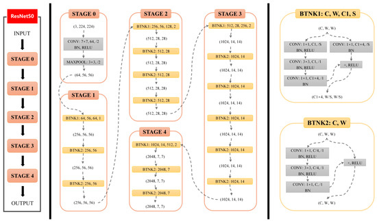
Figure 3. The network structure of TL-ResNet50.

2.4. Train

The training process was conducted in a laboratory environment, as detailed in Table 3. Specifically, a batch size of 32 and an initial learning rate of 0.001 were used to perform 100 model iterations, with each cycle consisting of 4500 batches. The training parameters can be found in Table 4.

Table 3. Lab environment.

Hardware Environment		Software Environment
Memory	16.0 GB	System	Windows 11
CPU	AMD Ryzen 9 5000 U (3.2 GHz)	Environment configuration	Pytorch-gpu 1.13 + Python 3.8.8 + cuda 11.7
Graphics card	NVIDIA GeForce GTX3060 (6G)

Table 4. Training parameters.

Related Parameter	Value	Meaning
Batch size	32	Number of pictures per training
Learning rate	0.001	Initial learning rate
Epoch	100	Training iteration times
CUDA	Enable	Comp

3. Results

3.1. TL-ResNet50 Training Results

Figure 4 illustrates the model’s loss function and accuracy in the training and test sets. As training began, the model’s accuracy quickly increased, reaching 95% after the first epoch and peaking at 99.4% in the 10th epoch. Ultimately, the optimal training accuracy reached 0.994 with a corresponding loss value of around 0.025. The average accuracy during the test phase was 0.998. The curve indicates that the model learned most of its features within the first 10 epochs and has a good recognition of the steel surface defects.

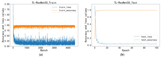
Figure 4. The TL-ResNet50 loss and accuracy change: (a) training phase; (b) testing phase. The blue line in the figure represents the change in the accuracy of the model, while the orange line represents the change in the loss value of the model. The x-axis represents the epoch of training, and the y-axis represents the values of accuracy and loss.

The ROC curve is a commonly used evaluation method for image classification, accurately depicting the specificity–sensitivity relationship of a given analysis method. The model’s overall accuracy can be intuitively determined by examining the ROC curve (Figure 5a), with closer curves indicating more accurate identification. Figure 5b presents a bar chart of the accuracy assessment index, visually depicting the correctness of several test set categories.

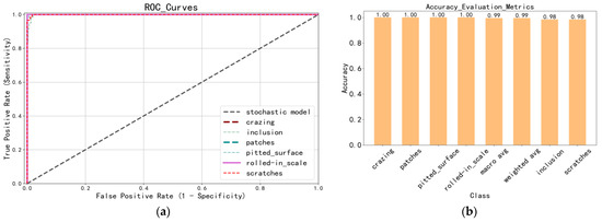
Figure 5. The model test set training results: (a) ROC curves of different categories; (b) bar chart of accuracy assessment indicators; the macro avg is the weighted average of each defect’s precision, recall, and F1-Score.

3.2. The Model Performance Comparative Analysis

To accurately evaluate the performance of the TL-ResNet50 model, this article compared it with three classic network models. The ResNet50 and TL-ResNet50 were used as control groups to assess the impact of TL on the model’s performance. It is worth noting that the VGG19 model has a more complex structure with the largest capacity, resulting in a greater demand for computing resources and time during training. Table 5 provides detailed parameters for all the models compared in this study.

Table 5. Parameter comparison of different models.

Models	In Features	Out Features	Bias	Transfer	Storage
TL-Resnet50	2048	6	True	True	97.9 MB
Resnet50	2048	6	True	False	44.6 MB
VGG19	4096	6	True	True	548 MB
AlexNet	4096	6	True	True	233 MB

Furthermore, this paper comprehensively assesses the model’s quality using various evaluation indicators, including accuracy (ACC), precision (P), recall (R), and F1-Score (F1). The formula for the evaluation indicators is defined as follows:

$$ACC=\frac{TP+TN}{TP+FP+FN+TN}$$

(4)

$$P=\frac{TP}{TP+FP}$$

(5)

$$R=\frac{TP}{TP+FN}$$

(6)

$$F1=2\cdot \frac{P\cdot R}{P+R}$$

(7)

The symbols in the formula represent the number of true positive (TP), false positive (FP), false negative (FN), and true negative (TN) cases in a binary classification problem.

In Figure 6, we present a comprehensive evaluation of several models using Formulas (4)–(7). The results show that TL-ResNet50 outperforms the other models, achieving higher values across all four assessment indicators within a shorter time. Furthermore, TL-ResNet50 exhibits less volatility and a smoother curve compared with those of ResNet50. Among the four models, ResNet50 displays the highest volatility and the slowest rate of convergence.

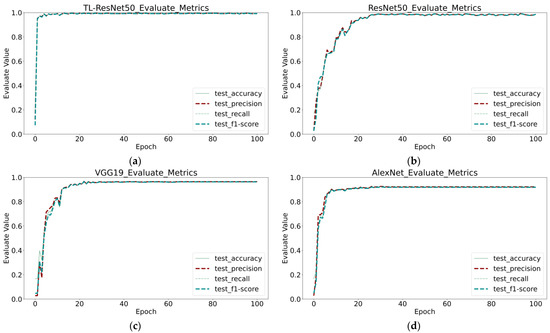
Figure 6. Comparison of evaluation indicators of four different models: (a) TL-ResNet50; (b) ResNet50; (c) VGG19; (d) AlexNet.

In Table 6, the AUC (area under curve) value represents the area between the ROC curve presented in Figure 7 and the coordinate axes, with a range of values from 0.5 to 1 indicating the ability of the model in distinguishing between positive and negative instances. Notably, numerous TL-ResNet50 AUC values are 1, indicating the model’s potential for practical applications. The average accuracy of TL-ResNet50, ResNet50, VGG19, and AlexNet, were 99.44, 98.06, 96.67, and 92.50%, respectively.

Table 6. Comparison of evaluation indexes of each model.

Class	Models	P	R	F1	ACC	AUC
Crazing	TL-Restnet50	100%	100%	100%	100%	1
	Restnet50	100%	100%	100%	100%	1
	VGG19	100%	100%	100%	100%	1
	AlexNet	85.71%	100%	92.31%	100%	0.99
Inclusion	TL-Restnet50	98.33%	98.33%	98.33%	98.33%	1
	Restnet50	93.44%	95.00%	94.21%	95.00%	0.999
	VGG19	98.28%	95.00%	96.61%	95.00%	0.996
	AlexNet	96.36%	88.33%	92.17%	88.33%	0.998
Patches	TL-Restnet50	100%	100%	100%	100%	1
	Restnet50	98.36%	100.00%	99.17%	100.00%	1
	VGG19	93.75%	100%	96.77%	100%	1
	AlexNet	100%	100%	100%	100%	1
Pitted surface	TL-Restnet50	100%	100%	100%	100%	1
	Restnet50	96.77%	100.00%	98.36%	100.00%	0.999
	VGG19	96.30%	86.67%	91.23%	86.67%	0.993
	AlexNet	86.96%	66.67%	75.47%	66.67%	0.975
Rolled-in scale	TL-Restnet50	100%	100%	100%	100%	1
	Restnet50	100%	100%	100%	100%	1
	VGG19	95.24%	100%	97.56%	100%	0.999
	AlexNet	90.91%	100%	95.24%	100%	0.998
Scratches	TL-Restnet50	98.33%	98.33%	98.33%	98.33%	1
	Restnet50	100.00%	93.33%	96.55%	93.33%	0.999
	VGG19	96.72%	98.33%	97.52%	98.33%	0.998
	AlexNet	95.24%	100%	97.56%	100%	1
Macro avg	TL-Restnet50	99.44%	99.44%	99.44%	99.44%	1
	Restnet50	98.10%	98.06%	98.05%	98.06%	0.999
	VGG19	96.71%	96.67%	96.62%	96.67%	0.998
	AlexNet	92.53%	92.50%	92.13%	92.50%	0.995
Weighted avg	TL-Restnet50	99.44%	99.44%	99.44%	99.44%	1
	Restnet50	98.10%	98.06%	98.05%	98.06%	0.999
	VGG19	96.71%	96.67%	96.62%	96.67%	0.998
	AlexNet	92.53%	92.50%	92.13%	92.50%	0.995

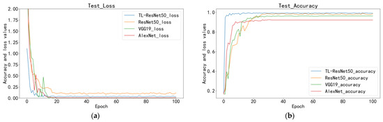
Figure 7. Comparison of the four models: (a) test loss; (b) test accuracy.

All four models exhibit high recognition performance in identifying crazing, patch, rolled-in scale, and scratch defects, with the TL-ResNet50 model exhibiting the best evaluation metrics among them. This indicates that these defects have significant feature information. However, there are significant evaluation metric differences among the four models in identifying inclusion and pitted surface defects. In particular, the AlexNet model exhibits poor recognition performance, with a recall rate and ACC index of only 66.77% for identifying pitted surface defects, while the VGG19 model also shows large fluctuations in its recognition performance for this defect. We will employ interpretable analysis methods in the following section to further investigate the reasons behind the poor recognition performance of these models.

3.3. Rate of Convergence Analysis

Figure 7 compares the accuracy and loss values of the four models in the test set. Although all models can converge within 100 cycles, their convergence time and accuracy significantly vary. During the training phase, TL-ResNet50 exhibits much better convergence than other models, reaching a total accuracy of 95% after only the first cycle, indicating that this model can rapidly recognize images. VGG19 exhibits the slowest convergence speed, achieving a somewhat stable but lower level of accuracy after 30 cycles. AlexNet displays the lowest accuracy and the slowest convergence rate. The ResNet50 model, which was not utilized for TL, has the highest loss value among the four models and converges considerably more slowly than the other TL models. In comparison, TL-ResNet50 shows the fastest reduction in loss value, remains at a lower level throughout the entire process, and consistently maintains higher accuracy than the other models.

Figure 8 illustrates the accuracy and loss values of TL-ResNet50, ResNet50, VGG19, and AlexNet during the training phase. The K-fold cross-validation method was employed, with the mean of five training results presented in the figure. Notably, AlexNet displays significant variations during training, indicating its lowest level of stability. VGG19 exhibits the slowest convergence speed and the highest initial value. Regarding convergence and accuracy, ResNet50 without TL also performs worse than the TL-ResNet50 model. In comparison, the TL-ResNet50 model’s performance can be fully demonstrated by mutually verifying the training set and test set curves.

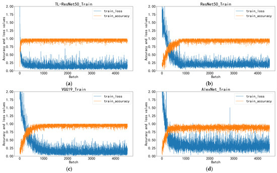
Figure 8. Comparison of the four models: (a) TL-ResNet50; (b) ResNet50; (c) VGG19; (d) AlexNet.

3.4. TL Comparison

To improve the generalization and robustness of the network, this paper used the ResNet50 pre-training model based on the ImageNet dataset. The confusion matrix in Table 7 shows that the TL-ResNet50 model has a strong overall identification rate, with only one misidentified case. In the testing phase, the ResNet50 model shows worse identification performance, with three inclusions and two scratches incorrectly identified. Figure 9 demonstrates that TL can significantly enhance the model’s convergence speed and reduce its loss value. The average accuracy of the TL-ResNet50 model with TL reaches 99.4%, surpassing ResNet50 (98.05%). These results indicate that TL can significantly enhance the model’s convergence speed and reduce the model’s loss value.

Table 7. Confusion matrix of TL and non-TL.

Method	Actual Category	Prediction Category
		Crazing	Inclusion	Patches	Pitted Surface	Rolled-in Scale	Scratches	Total
TL-ResNets50	Crazing	60	0	0	0	0	0	60
	Inclusion	0	59	0	0	0	1	60
	Patches	0	0	60	0	0	0	60
	Pitted surface	0	0	0	60	0	0	60
	Rolled-in scale	0	0	0	0	60	0	60
	Scratches	0	1	0	0	0	60	60
ResNets50	Crazing	60	0	0	0	0	0	60
	Inclusion	0	57	0	2	0	1	60
	Patches	0	0	60	0	0	0	60
	Pitted surface	0	0	0	60	0	0	60
	Rolled-in scale	0	0	0	0	60	0	60
	Scratches	0	2	0	0	0	58	60

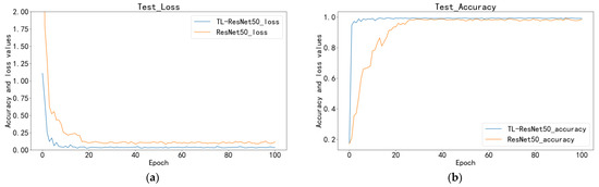
Figure 9. Comparison of transfer and non-TL: (a) test loss; (b) test accuracy.

3.5. Forecast Results Display and Explanatory Analysis

Finally, six common defects from the testing concentration were randomly selected (Figure 10), and different models’ defect recognition performance was compared.

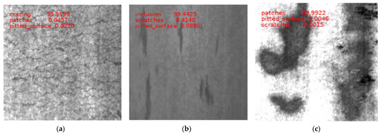
Figure 10. The confidence degree of surface flaws in six types of steel: (a) crazing; (b) inclusion; (c) patches; (d) pitted surface; (e) roll-in scale; (f) scratches. The upper left picture indicates the type of defect identified by the model, represented by the first text, followed by the confidence level of that defect type.

3.6. Explanatory Analysis

Research has shown the high accuracy of the TL-ResNet50 model in identifying surface defects on steel. However, due to a limited understanding of CNN model mechanisms, they often remain “black boxes” [17]. This study uses Gradient-weighted Class Activation Mapping++ (Grad-CAM++) [30] to conduct an interpretable analysis on TL-ResNet50, VGG19, and AlexNet models. By examining their defect recognition logic, the study sheds light on their focus on different defect types. Grad-CAM++ enhances the feature visualization by using multiple convolutional layers and global average pooling to generate a heat map that reflects the position and shape of defect images. Figure 11 illustrates the five-step identification process.

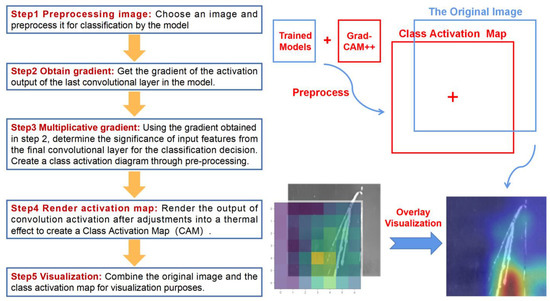
Figure 11. CAM visualization-specific steps and processes.

As shown in Figure 12, TL-ResNet50, VGG19, and AlexNet models were utilized to identify six types of surface defects on steel, followed by interpretable analysis using the Grad-CAM++ algorithm. Results show that due to the low number of convolutional layers in AlexNet, its identification performance is poor, failing to learn more general defect features and exhibiting inaccurate position recognition for the crazing, inclusion, pitted surface, and roll-in scale defects. Although VGG19 has greatly improved its recognition accuracy compared with AlexNet, it still falls short of TL-ResNet50 in comprehensive defect-type recognition. TL-ResNet50 exhibits the best recognition performance among the five defects, accurately identifying both the location and shape of the defects and demonstrating significant advantages over other models.

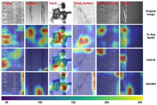
Figure 12. The interpretable analysis of six types of surface defects on steel using TL-ResNet50, VGG19, and AlexNet models in combination with Grad-CAM++. The color values represented in the figure indicate that the larger the value, the greater the impact on the model’s prediction results, indicating the most significant defect features.

The VGG19 and AlexNet models have convolutional layers before the global average pooling layer, which cannot directly output feature maps. Only the last layer global average pooling (GAP) can output images. In contrast, TL-ResNet50 has residual connections, enabling information flow through skip connections and outputting four different resolution feature maps. This allows TL-ResNet50 to extract more comprehensive feature information. When using Grad-CAM++, we were unable to perform in-depth feature analysis for the VGG19 and AlexNet models, while for the TL-ResNet50 model, this leads to a better understanding of network decision making.

Specifically, TL-ResNet50 has four layers of output (layer 1–layer 4), each corresponding to the feature information of the four convolutional layers in the model structure. From Figure 13, it can be observed that the defect features extracted by the first and second convolutional layers are relatively localized, focusing on low-level features such as the texture and edges of the object. Therefore, the generated heat map mainly marks the local area of the defects. The feature extracted by the third convolutional layer is more global, focusing on the shape and structure of the overall defect. The feature extracted by the fourth convolutional layer is more abstract, capturing higher-level semantic information but is also susceptible to overfitting, resulting in errors in the heat map.

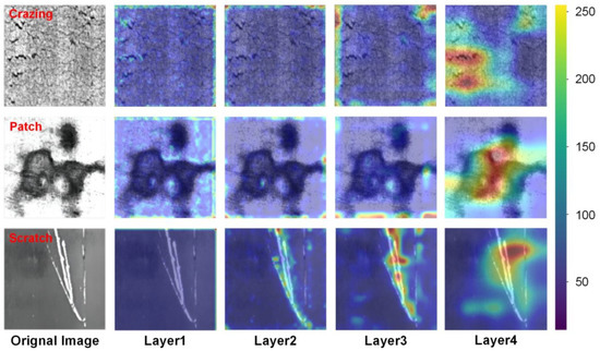
Figure 13. The Grad-CAM++ images generated by TL-ResNet50 for three types of defects (crazing, patch, and scratch). The color values in the image correspond to the degree of influence on the prediction results, whereby larger values indicate more significant defective features.

For example, when analyzing scratch defect images using Grad-CAM++, it was found that the heat map generated by the third layer is significantly more accurate than that generated by the fourth layer. This may be due to the fewer interferences present in the scratch defect image and the more noticeable defect features where good recognition accuracy can be achieved after three convolutional operations. However, after the fourth convolutional operation, the model did not learn better feature information but instead extracted more abstract features, leading to overfitting. Therefore, when using Grad-CAM++ for interpretability analysis, weight allocation of feature maps at different levels needs to be considered to obtain more accurate visualization results.

4. Conclusions

This article utilizes TL to enhance steel surface defect recognition by transferring feature extraction abilities learned from ImageNet. K-fold cross-validation effectively tests the model throughout the training process, improving its generalization performance. Combining the Adam algorithm with decreasing learning rate swiftly converges the model within five cycles, achieving an accuracy of over 99.4% and a low loss rate of 0.025. Multiple evaluation indicators show that TL-ResNet50 outperforms other neural network models, with many AUC indexes of 1, indicating the model’s excellent application value. This study suggests that TL-ResNet50 has great potential for practical applications in steel surface defect identification and emphasizes the importance of considering weight allocation when using Grad-CAM++ for interpretability analysis. Additionally, the study highlights different defect recognition focuses among TL-ResNet50, VGG19, and AlexNet models. Using the weak supervision method enhances result visualization’s intuitiveness and simplicity, with low computer performance requirements and a lightweight layout.

References

- Ghorai, S.; Mukherjee, A.; Gangadaran, M.; Dutta, P.K. Automatic defect detection on hot-rolled flat steel products. IEEE Trans. Instrum. Meas. 2013, 62, 612–621. [Google Scholar] [CrossRef]
- Shi, T.; Kong, J.; Wang, X.; Liu, Z.; Zheng, G. Improved sobel algorithm for defect detection of rail surfaces with enhanced efficiency and accuracy. J. Cent. South. Univ. 2016, 23, 2867–2875. [Google Scholar] [CrossRef]
- Jeon, Y.; Yun, J.; Choi, D.; Kim, S.W. Defect detection algorithm for corner cracks in steel billet using discrete wavelet transform. In Proceedings of the ICROS-SICE International Joint Conference, Fukuoka, Japan, 18–21 August 2009; pp. 2769–2773. [Google Scholar]
- Hu, H.; Liu, Y.; Liu, M.; Nie, L. Surface Defect Classification in Large-scale Strip Steel Image Collection via Hybrid Chromosome Genetic Algorithm. Neurocomputing 2016, 181, 86–95. [Google Scholar] [CrossRef]
- Tang, B. Steel Surface Defect Recognition Based on Support Vector Machine and Image Processing. China Mech. Eng. 2011, 22, 1402–1405. [Google Scholar]
- Gong, R.; Liu, L. Steel surface defects recognition based on multi-label classifier with hyper-sphere support vector machine. In Proceedings of the Control and Decision Conference (CCDC), Chongqing, China, 28–30 May 2017; pp. 3276–3281. [Google Scholar]
- Choi, D.C.; Jeon, Y.J.; Lee, S.J.; Yun, J.P.; Kim, S.W. Algorithm for detecting seam cracks in steel plates using a Gabor filter combination method. Appl. Opt. 2014, 53, 4865–4872. [Google Scholar] [CrossRef]
- Ashour, M.W.; Khalid, F.; Halin, A.A.; Abdullah, L.N.; Darwish, S.H. Surface defects classification of hot-rolled steel strips using multi-directional Shearlet features. Arab. J. Sci. Eng. 2018, 44, 2925–2932. [Google Scholar] [CrossRef]
- Song, K.; Meng, Q.; Yan, Y. An End-to-End Steel Surface Defect Detection Approach via Fusing Multiple Hierarchical Features; Loughborough University: Loughborough, UK, 2019; Available online: https://hdl.handle.net/2134/12249215.v1 (accessed on 5 December 2022).
- Hao, Z.; Wang, Z.; Bai, D.; Tao, B.; Tong, X.; Chen, B. Intelligent Detection of Steel Defects Based on Improved Split Attention Networks. Front. Bioeng. Biotechnol. 2022, 9, 810876. [Google Scholar] [CrossRef]
- Luo, Q.; Fang, X.; Liu, L.; Yang, C.; Sun, Y. Automated Visual Defect Detection for Flat Steel Surface: A Survey. IEEE Trans. Instrum. Meas. 2020, 69, 626–644. [Google Scholar] [CrossRef]
- Pan, S.J.; Tsang, I.W.; Kwok, J.T.; Yang, Q. Domain adaptation via transfer component analysis. IEEE Trans. Neural Netw. 2011, 22, 199–210. Available online: http://ieeexplore.ieee.org/abstract/document/5640675/ (accessed on 6 December 2022). [CrossRef]
- Wu, H.; Lv, Q. Hot-Rolled Steel Strip Surface Inspection Based on Transfer Learning Model. J. Sens. 2021, 2021, 6637252. [Google Scholar] [CrossRef]
- Bouguettaya, A.; Mentouri, Z.; Zarzour, H. Deep ensemble Transfer Learning-based approach for classifying hot-rolled steel strips surface defects. Int. J. Adv. Manuf. Technol. 2023, 125, 5313–5322. [Google Scholar] [CrossRef]
- Wan, X.; Zhang, X.; Liu, L. An Improved VGG19 Transfer Learning Strip Steel Surface Defect Recognition Deep Neural Network Based on Few Samples and Imbalanced Datasets. Appl. Sci. 2021, 11, 2606. [Google Scholar] [CrossRef]
- Zhang, Y.; Tiňo, P.; Leonardis, A.; Tang, K. A Survey on Neural Network Interpretability. IEEE Trans. Emerg. Top. Comput. Intell. 2021, 5, 726–742. [Google Scholar] [CrossRef]
- Szegedy, C.; Zaremba, W.; Sutskever, I.; Bruna, J.; Erhan, D.; Goodfellow, I.; Fergus, R. Intriguing properties of neural networks. arXiv 2013, arXiv:1312.6199. [Google Scholar]
- Nguyen, A.; Yosinski, J.; Clune, J. Deep neural networks are easilyfooled: High confidence predictions for unrecognizable images. In Proceedings of the IEEE Conference on Computer Vision and Pattern Recognition, Boston, MA, USA, 7–12 June 2015. [Google Scholar]
- Lipton, Z.C. The Mythos of Model Interpretability. arXiv 2016, arXiv:1606.03490. [Google Scholar]
- Doshi-Velez, F.; Kim, B. Towards A Rigorous Science of Interpretable Machine Learning. arXiv 2017, arXiv:1702.08608. [Google Scholar]
- Guidotti, R.; Monreale, A.; Ruggieri, S.; Turini, F.; Giannotti, F.; Pedreschi, D. A survey of methods for explaining black box models. ACM Comput. Surv. (CSUR) 2018, 51, 1–42. [Google Scholar] [CrossRef]
- Alex Krizhevsky, I.S.A.G. ImageNet classification with deep convolutional neural networks. Commun. ACM 2017, 2017, 84–90. [Google Scholar] [CrossRef]
- Karen Simonyan, A.Z. Very Deep Convolutional Networks for Large-Scale Image Recognition. arXiv 2015, arXiv:1409.1556. [Google Scholar]
- He, K.; Zhang, X.; Ren, S.; Sun, J. Deep residual learning for image recognition. In Proceedings of the IEEE Conference on Computer Vision and Pattern Recognition, Las Vegas, NV, USA, 27–30 June 2016; pp. 770–778. [Google Scholar]
- He, Y.; Song, K.; Meng, Q.; Yan, Y. An End-to-end Steel Surface Defect Detection Approach via Fusing Multiple Hierarchical Features. IEEE Trans. Instrum. Meas. 2020, 69, 1493–1504. [Google Scholar] [CrossRef]
- Wong, T.-T.; Yeh, P.-Y. Reliable Accuracy Estimates from k-Fold Cross Validation. IEEE Trans. Knowl. Data Eng. 2020, 32, 1586–1594. [Google Scholar] [CrossRef]
- Glorot, X.; Bordes, A.; Bengio, Y. Deep Sparse Rectifier Neural Networks. In Proceedings of the 14th International Conference on Artificial Intelligence and Statistics (AISTATS), Ft. Lauderdale, FL, USA, 11–13 April 2011. [Google Scholar]
- Kingma, D.P.; Ba, J. Adam: A method for stochastic optimization. arXiv 2014, arXiv:1412.6980. [Google Scholar]
- Jamin, A.; Humeau-Heurtier, A. (Multiscale) Cross-Entropy Methods: A Review. Entropy 2020, 22, 45. [Google Scholar] [CrossRef]
- Chattopadhay, A.; Sarkar, A.; Howlader, P.; Balasubramanian, V.N. Grad-CAM++: Generalized Gradient-Based Visual Explanations for Deep Convolutional Networks. In Proceedings of the 2018 IEEE Winter Conference on Applications of Computer Vision (WACV), Lake Tahoe, NV, USA, 12–15 March 2018; pp. 839–847. [Google Scholar] [CrossRef]
Disclaimer/Publisher’s Note: The statements, opinions and data contained in all publications are solely those of the individual author(s) and contributor(s) and not of MDPI and/or the editor(s). MDPI and/or the editor(s) disclaim responsibility for any injury to people or property resulting from any ideas, methods, instructions or products referred to in the content. |
© 2023 by the authors. Licensee MDPI, Basel, Switzerland. This article is an open access article distributed under the terms and conditions of the Creative Commons Attribution (CC BY) license (https://creativecommons.org/licenses/by/4.0/).