Multizone Leak Detection Method for Metal Hose Based on YOLOv5 and OMD-ViBe Algorithm

Abstract

It is necessary to determine the location and number of leaks in a pipeline in time to repair it, thus reducing economic losses. A multizone leakage detection method based on the YOLOv5 and OMD-ViBe algorithm is proposed to detect the metal hose’s location and leakage rate. The deep learning model of YOLOv5 is used to accurately recognize the zone of the metal hose for the region of interest rectification. The multiframe averaging method is applied to construct the initial background of the video frames. The OTSU algorithm based on the background difference method and the adaptive threshold of the maximum intraclass and interclass variance ratio method is used to improve the recognition rate of bubbles and reduce the influence of illumination change. In a comparison with the existing algorithms, the experimental results showed that OMD-ViBe improves the F-measure by 1.79–16.41% and the percentage of misclassification by 0.003–0.165%. Analysis of the pressure data indicated a comprehensive leakage error reduction of 1.53–25.19%, which can meet the requirements of metal hose leakage detection.

1. Introduction

Air tightness testing is widely used in industry and is an essential standard for evaluating metal hoses’ safety and quality. Products should be tested for leaks before leaving the factory according to the standards set by the industry. Various methods have been applied to leak detection, such as pressure detection, ultrasonic detection, infrared thermal imaging detection and machine vision.

Leak detection can be detected by pressure changes, flow noise and image information. Li et al., Yang et al., Shi et al. and Juan et al. located the leakage position and quantified leakage volume based on the pressure change [1,2,3,4]. If more than one leakage occurs, finding it becomes easier. Song et al., Zhou et al., Lang et al., Lyu et al., Quy et al., Li and Xue et al. located leakage position by detecting flow noise [5,6,7,8,9,10,11]. Flow noise can overwrite leak point information and interfere with leak detection results. Wang et al., Guan et al., Yu et al., Penteado et al., Wang et al. and Jadin et al. used infrared thermal imaging to locate the leakage position [12,13,14,15,16,17,18]. The infrared thermal image detection method requires there to be a temperature difference between the leakage media and the environment.

At present, deep learning is widely used in the field of ROI recognition due to its high recognition accuracy and high detection speed, and deep learning is being increasingly applied to image detection. Ren et al. and He et al. used two-stage target detection methods, but the detection speed needed to be faster [19,20]. Subsequently, Redmon et al. [21], Berg et al. [22] and Nepal al. [23] compared the two-stage detection methods and then improved the detection speed using the one-stage target detection method [21,22,23]. Based on the extracted ROI area, it is possible to continually identify the leaking bubbles in the area. Pan et al. obtained bubbles at the leaky point of the underwater confinement device using machine vision [24]. They extracted the bubble contour of the leaky end using a interframe difference algorithm combined with edge detection. Trunzer et al. combined infrared video data and machine vision techniques to extract frame feature blocks using principal component analysis and removed them with the K nearest neighbor method to classify the frame feature blocks and detect and locate the leakage point of liquid pipes [25]. Saworski and Zielinski combined a visual flow-splitting strategy with the Horn–Schunck algorithm to detect underwater bubbles and estimate the bubble size [26]. Several of the above machine vision methods use single-frame image segmentation methods to overcome the problem of ignoring the concentration of bubbles that are difficult to detect when the leakage rate is too fast.

Some researchers have proposed using the image information in video to detect leaks, which has a better detection effect than does the abovementioned method of using single-frame image information. Furthermore, Gao et al. used the background modeling algorithm to improve the bubble recognition efficiency using the video capture data method [27]. The background modeling algorithm is an image processing algorithm applied when significant differences between the current frame and the background model are shown, which generally includes the Gaussian mixture algorithm, ViBe algorithm, PBAS algorithm, etc. [28,29,30,31,32]. The ViBe algorithm proposed by Olivier Barnich et al., among other background modeling algorithms, is widely used as one of the features of faster and more accurate detection of moving targets.

Several researchers have used improvements of the ViBe algorithm in target detection. Zhou et al. improved PWC detection by inputting image depth information into the background model [33]. Qin et al. applied ViBe combined with the frame difference method to a vehicle detection system to remove the shadowing problem in ViBe detection [34]. Lyu et al. proposed a ViBe and EfficientNetB0 combination algorithm for leak identification to improve detection accuracy [35]. Dai and Yang proposed a ViBe adaptive threshold calculation method based on temperature field offset to eliminate the noise in the background and a round modeling method and threshold segmentation calculation value of the ViBe algorithm to improve the detection speed [36]. The abovementioned background model still had a poor detection effect on leak bubbles, so the ViBe algorithm was improved to improve leak detection performance.

The goal of this work is to provide a solution for metal hose leak rate calculation and leak location based on OMD-ViBe and pressure analysis. Different types and sizes of metal hose leaks affect bubble detection. The framework mentioned can be used for different types and sizes of metal hoses. In order to reduce the interference of the nonleakage area, YOLOv5 is used to extract the metal hose ROI area. In addition, it is proposed that OMD-ViBe uses multiframe average initialization background to eliminate the false detection caused by impurities or bubbles in the first frame of the video and uses the difference idea combined with OTSU and the maximum intraclass variance ratio method to calculate the adaptive threshold to improve the bubble detection effect. The multipoint leakage rate is calculated based on OMD-ViBe combined with pressure data and the foreground point frequency calculation method. The leakage location is realized by using the frequency superposition of the foreground points combined with the central moment method. Finally, the metal hose leak detection method based on YOLOv5 and OMD-ViBe can effectively improve the leak detection effect.

The remainder of the paper is organized as follows. In Section 2, the formula of YOLOV5 region correction is given, and the improvement of the OMD-ViBe algorithm, the calculation method of foreground point frequency and the central moment leakage location method are presented. The metal hose leakage detection results are provided in Section 3. Finally, concluding remarks and potential future work are given in Section 4.

2. Leak Detection Methods

2.1. Detection Process

Pressure detection and machine vision are utilized to detect the leakage rate and leak location of the metal hose. Figure 1 shows the diagram of the metal hose leakage detection algorithm, including the leak bubble, recognition, leak location detection and leak rate calculation. To detect the leakage in multiple zones of the metal hose, the total video of the metal hose should be captured and recorded via camera. The ROI region of the metal hose is extracted to decrease the calculation burden based on the YOLOv5 model. The Mosaic image enhancement method balances and enlarges the data to improve the model’s generalization capability in YOLOv5. Then, a target area correction is adopted to extract the metal hose area, as shown in Figure 2. Based on the oblique ROI extraction of YOLOv5, the foreground calculation method of the background modeling algorithm is adopted to identify foreground points. Then, centroid coordinates are extracted based on the frequency of foreground points to obtain the location of the leakage area. Finally, e the collected pressure data values are combined with the frequency of foreground points in the leakage area for the multipoint leakage volume calculation.

2.2. ROI Rectification

The ROI area partially corresponds to the metal hose. The detection frame is too large when the metal hose is tilted. The ROI area is corrected to conform to the tilted metal hose, as shown in Figure 2. The yellow box represents the nut area. The red box is the net sleeve area. When there is a deviation in the pressure vessel in the prediction box, as shown in Figure 2b, the center lines of the yellow and red boxes form a certain deflection angle θ, and the red ROI area is rotated counterclockwise according to the deflection angle to correct the target box. The ROI correction formula is as follows:

$$\left\{\begin{array}{c}{x}_{Hose}=\frac{x_2-x_1}{2}+x_1,y_{Hose}=\frac{y_2-y_1}{2}+y_1\\ x_{Nut}=\frac{x_4-x_3}{2}+x_3,y_{Nut}=\frac{y_4-y_3}{2}+y_3 \end{array}\right.,$$

(1)

$$\theta ={\tan }^{-1}\frac{y_{Nut}-y_{Hose}}{x_{Nut}-x_{Hose}},$$

(2)

$$\left\{\begin{array}{c}{x}_1^{\prime }=\left(x_1-x_{Hose}\right)\ast \cos \theta -\left(y_1-y_{Hose}\right)\ast \sin \theta +x_{Hose}\\ y_1^{\prime }=\left(x_1-x_{Hose}\right)\ast \sin \theta +\left(y_1-y_{Hose}\right)\ast \cos \theta +y_{Hose}\\ x_2^{\prime }=\left(x_2-x_{Hose}\right)\ast \cos \theta -\left(y_2-y_{Hose}\right)\ast \sin \theta +x_{Hose}\\ y_2^{\prime }=\left(x_2-x_{Hose}\right)\ast \sin \theta +\left(y_2-y_{Hose}\right)\ast \cos \theta +y_{Hose}\end{array}\right..$$

(3)

2.3. OMD-ViBe

After the ROI region obtained, background subtraction can be used to recognize the bubbles, and the proposed method improves ViBe to better recognize bubbles. OMD-ViBe improves the background initialization and fixed threshold calculation in the ViBe algorithm, resulting in improved recognition performance compared to other algorithms.

2.3.1. ViBe Theory

During the process of background initialization, the ViBe algorithm randomly extracts M pixel values as the background model of each pixel in the $N_G\left(x,y\right)$ domain centered on the pixel by traversing each pixel in the first frame image.

$$B{K}_M=f\left(x,y\right)|\left(x,y\right)ϵN_G\left(x,y\right).$$

(4)

where $B{K}_M$ is the established background model.

In the step of foreground detection, the Euclidean distance between the corresponding pixel points can be found by comparing the following image pixel values with the background model. The number of sample points is counted, as the Euclidean distance is less than the fixed threshold R in Figure 3. If the number of sample points is less than the set threshold, the pixel is determined as the foreground point; otherwise, it is determined as the background point. The determination formula is as follows:

$$N_i\left(x,y\right)=\left\{\begin{array}{c}{N}_i\left(x,y\right)+1, if dist\left(f^i\left(x,y\right),B{K}_M\right)<R \\ N_i\left(x,y\right)+0, else \end{array}\right.,$$

(5)

$$f^t\left(x,y\right)=\left\{\begin{array}{c}D{B}_i\left(x,y\right)=foreground, if N_i\left(x,y\right)<T\\ D{B}_i\left(x,y\right)=background,else \end{array}\right..$$

(6)

where $dist\left(f^i\left(x,y\right),B{K}_M^n\right)$ is the Euclidean distance between the image and the background model, R represents the fixed threshold, T represents the decision-matching value, and $N_i\left(x,y\right)$ represents the matching number of the coordinates corresponding to the background model.

The ViBe algorithm adopts a conservative update strategy with a random selection of pixels, which effectively guarantees the spatial consistency of neighborhood pixels. If the pixel is determined as the background point, there is a 1/φ probability of updating the background model $B{K}_M$; that is, the pixel value in the current image of $D{B}_i\left(x,y\right)$ is randomly replaced by $B{K}_M$.

$$\left(t,t+dt\right)={(\frac{\phi -1}{\phi })}^{\left(t+dt\right)-t}.$$

(7)

2.3.2. Improving ViBe

The traditional ViBe algorithm is prone to ghosting if moving bubbles are in the initial frame. Meanwhile, the water surface ripple can easily affect the detection resulting from image interference under the detection conditions of a metal hose. The originally fixed threshold R cannot adapt to this detection condition well. Therefore, this paper improves the background modeling and foreground detection part for the ViBe problem.

The traditional ViBe algorithm builds up a background sample library by the first frame, but if there are, for example, floating bubbles or impurities in the first frame, this can cause interference pixels in the background sample library and eventually lead to false detection. Therefore, we use the first n frames of the images to improve the background initialization: the first n frames of images are used to create a total image set, each pixel point in the metal hose picture is traversed, and the pixel values are randomly extracted on the corresponding neighborhood of the image set M times to form a background sample library $B{K}_M$. This library is expressed as follows:

$$B{K}_M=g_N(f^n\left(x,y\right)|\left(x,y\right)ϵN_G\left(x,y,M\right)),M=range\left(10\right)).$$

(8)

where $f^n\left(x,y\right)$ is the pixel value of the pixels in the neighbourhood extracted by all the pixes $\left(x,y\right)$ in the first n frames of the metal hose image, $N_G\left(x,y\right)$ is the neighborhood of the pixel $\left(x,y\right)$. $g_N\left(\ast \right)$ represents the execution of N times, and $range\left(\ast \right)$ represents the random number.

The main idea of the OTSU algorithm is to divide the image into background and foreground according to the gray characteristics so that the variance between background and foreground is the largest. However, the OTSU algorithm can easily misjudge the foreground point as the background in image segmentation. In this paper, the background model in the ViBe algorithm and the OTSU algorithm are combined to calculate the dynamic thresholds $T_1$ and $T_2$ by using the image difference idea. Additionally, the maximum intraclass and interclass variance ratio methods are introduced, and the threshold $T_3$ is calculated by using the characteristics of this method. The final dynamic threshold is derived by combining the thresholds with the calculation. The OTSU and the maximum intraclass and interclass variance ratio methods rely on the mean difference and variance to calculate the results via Formulas (9) and (10).

$$\left\{\begin{array}{c}{\mu }_1=\frac{1}{N_{C1}}{\displaystyle \sum }_{f\left(x,y\right)\in C1}f\left(x,y\right),{\sigma }_1^2={\displaystyle \sum }_{f\left(x,y\right)\in C1}{(f\left(x,y\right)-{\mu }_1)}^2\\ {\mu }_2=\frac{1}{N_{C2}}{\displaystyle \sum }_{f\left(x,y\right)\in C2}f\left(x,y\right),{\sigma }_2^2={\displaystyle \sum }_{f\left(x,y\right)\in C2}{(f\left(x,y\right)-{\mu }_2)}^2 \end{array}\right.,$$

(9)

$$p_1=\frac{N_{C1}}{N_{image}},p_2=\frac{N_{C2}}{N_{image}},$$

(10)

where $f\left(x,y\right)$ is the picture of the video, $C1$ belongs to the foreground set, $C2$ belongs to the background set, $N_{C1}$ is the number of foreground pixels, $N_{C2}$ is the number of background pixels, $N_{image}$ is the total number of pixels in the image, ${\mu }_1,{\mu }_2$ is $\mathrm{the}$ mean value, ${\sigma }_1^2,{\sigma }_2^2$ is the variance, and $p_1,p_2$ is the distribution probability.

Based on the maximum gray value and minimum gray value of the image, the maximum of $p_1{\sigma }_1^2+p_2{\sigma }_2^2$ is obtained by traversing the two value intervals, and the threshold TH calculated by the OTSU algorithm is accepted at this time. Then, $T_1$ and $T_2$ are computed using OTSU combined with the background model difference results and frame difference results. In the maximum intraclass and interclass variance ratio method, ${\mu }_1,{\mu }_2, {\sigma }_1^2,{\sigma }_2^2$ is used to calculate $S_1$ and $S_2$, and the ratio of $S_1$ to $S_2$ is searched from the minimum gray value to the maximum gray value to obtain $T_3$. The threshold obtained by $T_1$, $T_2$ and $T_3$ is used to adjust the parameters of the actual leakage detection image to acquire the final $R_i$. Finally, the dynamic threshold R_i distinguishes the front and back attractions. The formulae are as follows:

$$OTS{U}_{TH}={(p_1{\sigma }_1^2+p_2{\sigma }_2^2)}_{max},$$

(11)

$$\left\{\begin{array}{l}{T}_1=g_{OTSU}\left(\left|f_i-B{K}_N^n\right|\right) \\ T_2=g_{OTSU}\left(\left|f_i-f_{i-1}\right|\right) \end{array}\right.,$$

(12)

$$S_1=p_1\ast {\left({\mu }_1-\mu \right)}^2+p_2\ast {\left({\mu }_2-\mu \right)}^2,$$

(13)

$$S_2=p_1\ast {{\displaystyle \sum }}_{f\left(x,y\right)\in C1}{\left(N_{C1}-{\mu }_1\right)}^2+p_2\ast {{\displaystyle \sum }}_{f\left(x,y\right)\in C2}{\left(N_{C2}-{\mu }_2\right)}^2,$$

(14)

$$T_3={(\frac{S1}{S2})}_{max},$$

(15)

$$R_i=\alpha T_1+\beta T_2+\gamma T_3,$$

(16)

$$B{W}_i=\left\{\begin{array}{c}1 f_i\left(x,y\right)>R_i\\ 0 otherwise \end{array}\right..$$

(17)

where ${OTSU}_{TH}$ is the threshold calculated by OTSU, $f_i\left(x, y\right)$ is the i-th frame image, $S_1$ is the intraclass variance, $S_2$ is the interclass variance, $B{W}_i$ represents the foreground or background points obtained by combining the grayscale values of $T_1$, $T_2$ and $T_3$ determined for the current frame as represented by 1 and 0.

2.4. Foreground Frequency Calculation Method

The binary image generated by OMD-ViBe is utilized to compute the frequency of foreground points within each subregion. This involves summing up the frequency of changes in foreground points for each pixel coordinate within the subregion. The average frequency of changes $A_i$ is computed based on the number of images, and the subregions exhibiting excessive changes are filtered out using a threshold. The percentage of sub-regions exhibiting excessive changes is then computed to determine the extent of leakage. The formulae are as follows:

$$X_i^t={{\displaystyle \sum }}_{t\in \left[1,m\right]}I(f_{i,\left(x,y\right)}^t=foreground),$$

(18)

$$A_i=\frac{X_i^t\left(x,y\right)-{(X_i^t)}_{min}}{{(X_i^t)}_{max}-{(X_i^t)}_{min}},X_i^t\left(x,y\right)\in X_i^t,$$

(19)

$$F_i=I\left(A_i>\epsilon \right)\times {{\displaystyle \sum }}_{t\in \left(n,m\right]}I(f_{i,\left(x,y\right)}^t==255),$$

(20)

$$P_i=\frac{F_i}{\sum F_i}\in \left[0,1\right].$$

(21)

where m is the final frame number of the video, $X_i^t$ is the sum of the pixel change frequency of the subregion, $A_i$ is the average pixel change frequency of the subregion after the maximum normalization, $F_i$ is the frequency of the corresponding region, $P_i$ is the percentage of the leakage subregion, $I\left(\ast \right)$ is the conditional function when the conditions are met, and $I\left(\ast \right)$ = 1 or $I\left(\ast \right)$ = 0.

2.5. Leakage Point Location

The frequency distribution of the top attractions is obtained by $F_i$. By calculating the central moments of the frequency distribution of the front point, the coordinate points of the front point in the most densely distributed area of the image are obtained as follows:

$$\left\{\begin{array}{c}{I}_x=\frac{M_{10}}{M_{00}}\\ I_y=\frac{M_{01}}{M_{00}}\end{array}\right..$$

(22)

where $M_{00}$ is the set of pixel values in the region of $F_i$, $M_{10}$ is the set of x coordinates in the region of $F_i$, $M_{01}$ is the set of y coordinates in the region of $F_i$, and $I_x$ and $I_y$ are the centroid coordinates of the leakage region.

2.6. Leakage Calculation

As the inflation is completed, the holding pressure testing is performed. The pressure data are collected to obtain the pressure drop value during the holding process.

According to the ideal gas state, Equation (23) is as follows:

$$pV=mRT.$$

(23)

Which is converted to Equation (24)

$$m=\frac{pV}{RT}.$$

(24)

The gas mass before leakage and the gas mass after leakage are calculated as follows:

$$\Delta m=\frac{p_{1}V}{R{T}_1}-\frac{p_{2}V}{R{T}_2}.$$

(25)

Substituting the gas state equation yields Formula (26):

$$\Delta V=\frac{\Delta mR{T}_0}{p_0}.$$

(26)

The calculation result of the total leakage is obtained as follows:

$$Q=\frac{\Delta V}{\Delta t}.$$

(27)

Finally, when the total leakage and the leakage proportion of the subregion are known, the subregion leakage can be calculated as follows:

$$Q_i=Q\times P_i.$$

(28)

where $p$ is the pressure in the container, $V$ is the volume of the container, $m$ is the gas mass in the container, $R$ is the gas constant$, T$ is the temperature in the container, $T_0$ is the ambient temperature, $p_0$ is the atmospheric pressure, $Q$ is the leakage, and $\Delta t$ is the holding time.

3. Experiment and Results

The length of the two metal hoses in the experiment was 310 mm and 430 mm, as shown in Figure 4. The platform mainly consisted of the pressure-reducing valve, solenoid valve, electric proportional valve and pressure sensor (0–1 Mpa, accuracy of 0.01 %, gauge pressure, 24VDC). The data acquisition system included one control board (STM32F107) and a personal computer.

The experimental images were collected with an XW-200 color industrial camera. The camera’s complementary metal oxide semiconductor (CMOS) was 1/2.7″, and the effective pixel size was 200 w (1920 × 1080). In addition, the image processing was performed on a computer with the Windows 11 operating system using Opencv and PyTorch. To adequately handle the processing of the YOLOv5, the laptop used had a GeForce GPU T4 graphics processor. This proposed method’s training set includes 1000 self-made pictures and labels. Figure 5 is a representative picture of the training set, Figure 5a is taken from the side when the brightness is high, Figure 5b is taken from the front when the light is strong, Figure 5c is taken from the side when the brightness is low, and Figure 5d is taken when the brightness is low frontal shot. As shown in Figure 2, labels were set on the net sleeve part and the nut. respectively. The data set used in the moving target algorithm included 9000 frames of metal hose leakage original video as the moving target algorithm detection data set.

The platform works as follows: (1) The metal hose is connected with the gasket and the trachea; (2) After installation, the metal hose is placed in water; (3) The proportional valve and solenoid valve are opened to adjust the pressure. When the pressure value reaches a stable value, the image information is processed, and the pressure data are collected. (4) After the test time is completed, the solenoid valve is opened for pressure relief, and the air tightness test results are given in combination with the algorithm described in this paper.

3.1. Evaluation Index

The evaluation indexes of the YOLOv5 model and moving target algorithm mainly include mAP50, precision, recall, F-measure and percentage of wrong classification (PWC). The precision and recall rate index tends to be 1, and the F-measure is used as the comprehensive evaluation index of the precision and recall rate. The closer the error ratio is to 0, the better the effect. The indexes are defined as follows:

$$\mathrm{Precision}=\frac{\mathrm{TP}}{\mathrm{TP}+\mathrm{FP}},$$

(29)

$$\mathrm{Recall}=\frac{\mathrm{TP}}{\mathrm{TP}+\mathrm{FN}},$$

(30)

$$\mathrm{F}\text{-}\mathrm{measure}=2\ast \frac{\mathrm{Precision}\ast \mathrm{Recall}}{\mathrm{Precision}+\mathrm{Recall}},$$

(31)

$$\mathrm{PWC}=\frac{\mathrm{FP}+\mathrm{FN}}{\mathrm{TP}+\mathrm{FN}+\mathrm{FP}+\mathrm{TN}},$$

(32)

TP represents the number of foreground points detected correctly, TN represents the number of background points detected correctly, FP represents the number of background points mistakenly seen as foreground points, and FN represents the number of foreground points incorrectly identified as background points.

3.2. Experimental Results

3.2.1. YOLOv5 Results

This section analyzes and discusses the training results based on YOLOv5 under the self-made metal hose dataset. Figure 6 shows that the training accuracy and recall rate of YOLOv5 was 100 %, the mAP50 result was 99.5%, the detection speed with the YOLOv5 model was 30 FPS, and the detection with the YOLOv5 model could meet the detection requirements.

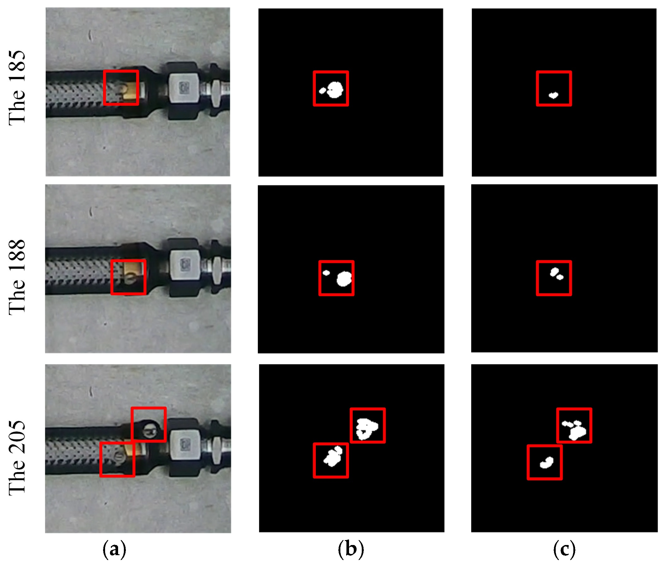
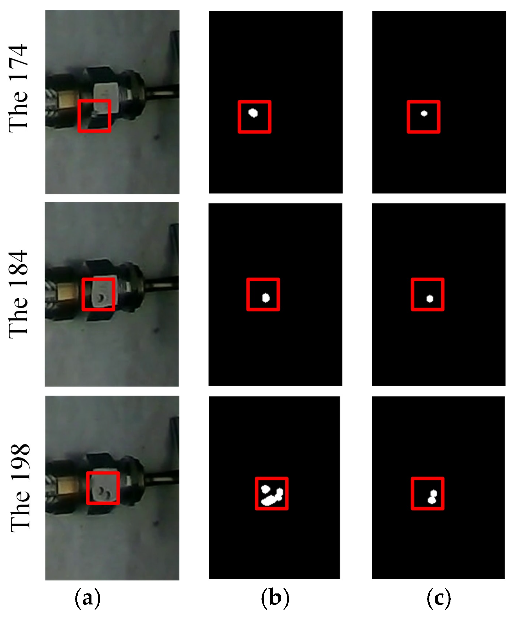
3.2.2. Bubble Recognition Based on OMD-ViBe

To find suitable values for the parameters $\alpha$, $\beta$ and $\gamma$, the image set with bubbles in 1000 frames under 0.4 Mpa pressure was extracted as the dataset for the optimization parameters of the particle swarm optimization algorithm (PSO), and the image frames with bubbles in the data were selected to calculate the results of the improved ViBe algorithm and the image frames using the F-measure values. The 1000 frames were used to find the optimal values of $\alpha$, $\beta$ and $\gamma$.

The particle swarm algorithm had 50 iterations and a population of 10, and the parameters $\alpha$, $\beta$ and $\gamma$ were optimized within [0.05,0.3]. The F-measure value was a combination of accuracy and recall, which was the target of the calculation and better reflects the comprehensive evaluation of the image algorithm. Finally, $\alpha$ = 0.188, $\beta$ = 0.05 and $\gamma$ = 0.05 were used as the optimized parameter values. The F-measure value obtained according to the PSO algorithm was 83.97%, as can be seen in Figure 7.

Table 1. Algorithm comparison results of 1000 frames.

Algorithm	Precision	Recall	F-Measure	PWC
ViBe	72.84%	87.87%	79.64%	0.113%
GMM	68.33%	87.88%	76.88%	0.096%
DPPratiMediod [30]	74.53%	79.17%	76.78%	0.111%
PBAS [31]	61.89%	97.65%	75.77%	0.165%
KNN	74.53%	79.17%	76.78%	0.111%
ViBeImp [32]	86.17%	78.54%	82.18%	0.084%
SigmaDelta	56.69%	98.59%	71.28%	0.201%
Adaptive Background Learning	51.74%	97.30%	67.56%	0.246%
Our method	80.88%	87.31%	83.97%	0.081%

presents the results of comparing OMD-ViBe with other algorithms after the particle swarm optimization algorithm was applied. After the accuracy, recall, F-measure and error rate were evaluated, it was evident that the OMD-ViBe algorithm outperformed ViBe in terms of F-measure and PWC, with an improvement of 4.33% and 0.049%, respectively. These findings demonstrate that the proposed OMD-ViBe algorithm in this paper represents a significant advancement in computing dynamic thresholds using the parameter values obtained through the particle swarm optimization algorithm for optimization.

To validate the efficacy of the parameters obtained from the optimization of 1000 frames in enhancing ViBe, tests were conducted on 8000 additional frames of data, which were divided into 8 intervals using every 1000 frames. The results, including the average accuracy, recall, F-measure and PWC, are presented in

Table 2. Algorithm average test results.

Algorithm	Precision	Recall	F-Measure	PWC
ViBe	81.64%	66.01%	71.12%	0.08%
GMM	68.49%	66.48%	60.58%	0.12%
DPPratiMediod	73.57%	85.10%	77.99%	0.08%
PBAS	62.64%	93.78%	73.21%	0.12%
KNN	66.48%	94.64%	76.85%	0.010%
ViBeImp	61.14%	66.75%	61.46%	0.11%
SigmaDelta	56.99%	97.08%	70.33%	0.15%
Adaptive Background Learning	59.22%	94.94%	71.43%	0.14%
Our method	85.47%	77.18%	81.11%	0.05%

. The findings indicate that the approach proposed in this paper provided an improvement in the F-measure for the test dataset as compared to the other algorithms.

In Figure 8, leak detection bubbles are denoted by red boxes in the diagram. When bubbles leak, the background subtraction algorithm recognizes the bubbles as former points of interest to distinguish them from nonbubble background points. To make it easier to compare the leak detection results of each image recognition algorithm, a local comparison is used as an intuitive way to compare the algorithms.

In Figure 9, the frames 186, 365, 570, 837 and 911 are shown to compare each algorithm. In the figure, white indicates that the target has been correctly detected, green indicates that the target has been misjudged as a nontarget, and red indicates that the actual nontarget has been underestimated as a target.

In frame 186, it can be observed that the traditional ViBe algorithm is susceptible to ghosting due to the slow movement of bubbles. This results in inconsistent detection outcomes with the target, leading to false detections. However, in frame 365, it is shown that PBAS and the adaptive background learning algorithms can detect many disturbing factors during bubble movement, which could be attributed to water lighting effects or image noise in the actual scenario. It can be concluded that the algorithm is highly resistant to interference and can further improve detection accuracy by eliminating the ghosting caused by slow bubbles.

This paper presents constructed videos depicting normal leakage and minor leakage, consisting of a total of 1000 frames per video. We propose the OMD-ViBe algorithm and conducted comparison experiments between the original ViBe algorithm and the improved version. The effectiveness of these algorithms was analyzed in each detection scenario based on two working conditions. The following section provides a detailed analysis of the impact of both algorithms in each scenario.

Figure 10 displays the results of normal leak detection, showcasing three frames of bubble movement at frames 185, 188 and 205 for comparison. Figure 10a presents the original video image, while Figure 10b,c show the detection outcomes of the OMD-ViBe algorithm, with the bubbles marked in red boxes for easier analysis. The figures reveal that the bubble profile obtained by the OMD-ViBe algorithm is more comprehensive than that of the original figure. This improvement is attributed to the dynamic threshold calculation method used by the OMD-ViBe algorithm, which has higher sensitivity to bubble appearance in the frame image, resulting in better detection outcomes.

Figure 11 presents the results of tiny-leak detection, with frames 174, 184 and 198 selected for comparison. Figure 11a displays the original video image, while Figure 11b,c present the detection outcomes of the OMD-ViBe algorithm. Both algorithms could detect the bubble to some extent, but it can be observed that in frame 198, Figure 11c has a false detection. This false detection is due to the ghosting phenomenon caused by the traditional ViBe algorithm when the bubble moves slowly, and the detected bubble foreground target is not updated in time, leading to false detection. However, the algorithm proposed in this paper effectively avoids this situation and accurately identifies the target.

To determine the frequency of each pixel point, the detection results of the OMD-ViBe and ViBe algorithms were overlaid on 1000 frames, and the calculation formulae outlined in Equations (18)–(21) were applied. The statistical outcomes are presented in Figure 12. Through a comparison of the results in Figure 12a,b and Figure 12c,d, it can be observed that the OMD-ViBe algorithm has a slightly higher frequency than does the ViBe for both the normal leakage and microleakage scenarios. This indicates that the OMD-ViBe algorithm detects bubbles corresponding to a higher number of former attractions, as shown in Figure 10 and Figure 11. Thus, these findings confirm the superior effectiveness of the OMD-ViBe algorithm in extracting bubble information.

Figure 13a displays the original map without any leakage, while Figure 13b shows the map with leakage points. Figure 13c,d demonstrate the effect of the ViBe and OMD-ViBe algorithms on the frequency superposition of former points of interest for normal and minor leakage scenarios, respectively. The superimposed plots have been normalized using Equation (19) to represent the highest and lowest frequencies within the image. The colors used to represent the normalized values are red for 0.8–1, yellow for 0.4–0.8 and blue for 0–0.4. Frequency counts between 0 and 0.4 mostly represent noise or false detections due to environmental interference and do not indicate the location of the leak. The closer the frequency count is to 1, the closer the leak is to the corresponding pixel point.

As seen in Figure 13c,d, excluding frequency counts above 0.2 could effectively eliminated noise in the background and false detections caused by environmental interference. The results can pinpoint the location of the leak with higher frequency counts, indicating the effectiveness of the overlay localization method for former points of interest.

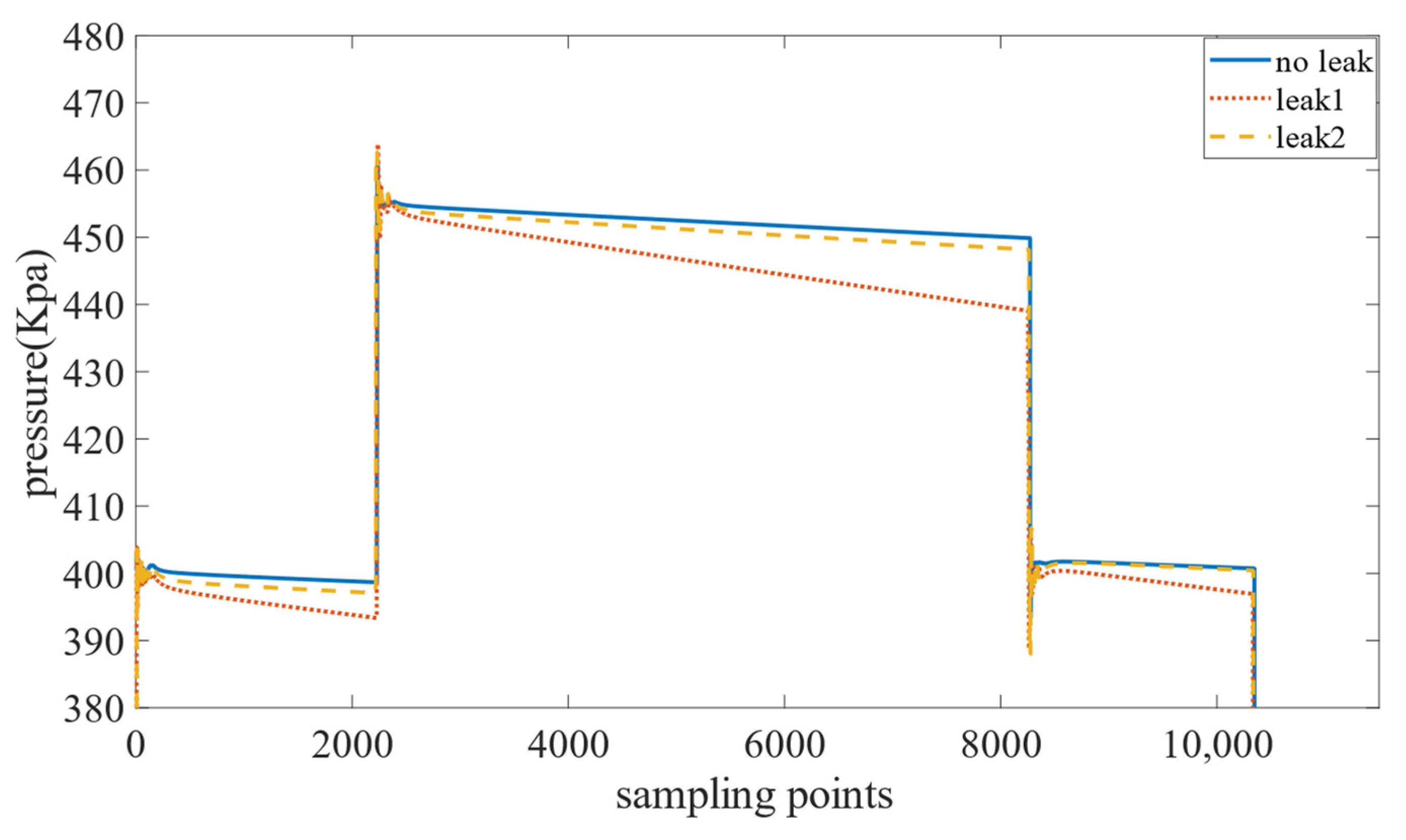
3.2.3. Leakage Calculation

This section presents a comparative experiment using nonleakage and leakage metal hoses to verify the accuracy of regional leakage calculation. The inner diameter of the leaking metal hose was 25.3 mm and the outer diameter was 32.3 mm. The test time included pressure data collected by the image within 9000 frames. The pressure data were divided into three stages, with the first and third stages representing the working pressure and the second stage representing the test pressure. Figure 14 illustrates the pressure data collected from the device and the leaky metal hose. The pressure data of the intact metal hose were also declining as a whole because the acquisition device itself had specific leakage. However, the pressure drop of the leaky metal hose was significantly higher, indicating that the metal hose’s leakage degree was more significant than was the acquisition device’s leakage. Therefore, using the pressure acquisition method proposed in this paper is feasible.

Table 3. Leak 1 and leak 2 test results.

Pressure (Mpa)	Leak 1 Pressure Drop (Pa)	Leak 2 Pressure Drop (Pa)	Leak 1 Leakage Rate (mL/min)	Leak 2 Leakage Rate (mL/min)
0.2	4652	1233	0.235	0.092
0.3	8259	2259	0.416	0.168
0.4	13,654	5322	0.688	0.397

shows the results of the separate tests for the leakage of pipe 1 and pipe 2 at 0.2 Mpa, 0.3 Mpa and 0.4Mpa.

Table 4. No leak and two leaks combined test results.

Pressure (Mpa)	No Leak Pressure Drop (Pa)	Combined Pressure Drop (Pa)	No Leak Leakage Rate (mL/min)	Combined Leakage Rate (mL/min)
0.2	2	2705	0.0007	0.338
0.3	3	4653	0.0011	0.581
0.4	6	8934	0.0021	1.116

shows the results of the leakage rate of the device itself and the simultaneous test of the leakage pipes 1 and 2. Each data group was measured five times to ensure the accuracy of the data.

In

Table 5. Leakage rate comparison between the proposed method and eight traditional methods.

Algorithm	Leak 1 Leakage Rate (mL/min)	Leak 2 Leakage Rate (mL/min)	Leak 1 Error	Leak 2 Error
ViBe	0.755	0.361	9.71%	9.01%
GMM	0.711	0.405	3.35%	2.00%
DPPratiMediod	0.635	0.481	7.76%	21.25%
PBAS	0.709	0.407	3.01%	2.58%
KNN	0.701	0.415	1.89%	4.53%
ViBeImp	0.757	0.359	9.98%	9.48%
SigmaDelta	0.699	0.417	1.58%	5.07%
Adaptive Background Learning	0.722	0.394	5.00%	0.85%
Proposed Method	0.685	0.431	0.37%	3.45%

, the algorithm in the Table 4 is used to calculate the foreground frequency of the leakage pipe. The leakage rate of different pipes was calculated according to the leakage rate calculated by the pressure and compared with the separate leakage pipe. It can be concluded that the comprehensive leakage error of pipe 1 and pipe 2 calculated by the foreground frequency of other algorithms was reduced by 1.53–25.19%. By considering the higher F-measure and PWC in Table 1, it can be concluded that the computed leakage is more accurate, which shows the algorithm’s effectiveness in this study.

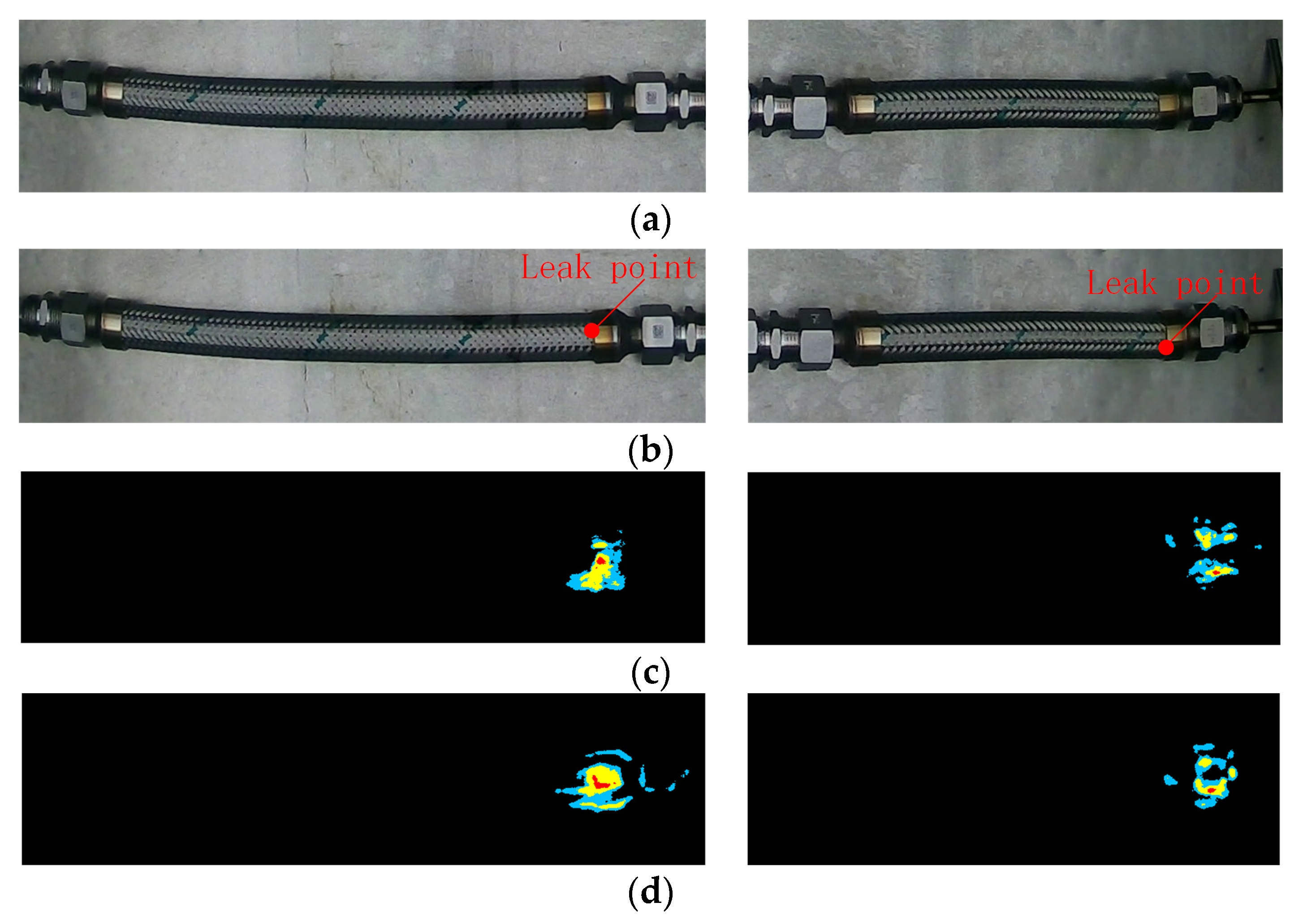
3.2.4. Leak Location

The length of the actual measurement tube 1 was 310 mm, and the size of tube 2 was 430 mm. The leakage points of the two were divided into 89.53% and 85.48% of the total tube length. As shown in

Table 6. Leakage rate comparison between the proposed method and eight traditional methods.

Algorithm	Leak 1 Location	Leak 2 Location	Leak 1 Error	Leak 2 Error
ViBe	91.97%	86.22%	2.44%	0.74%
GMM	80.12%	86.48%	9.41%	1%
DPPratiMediod	81.33%	86.88%	8.2%	1.53%
PBAS	91.16%	86.35%	1.63%	0.87%
KNN	85.54%	86.48%	3.99%	1%
ViBeImp	91.16%	87.14%	1.63%	1.66%
SigmaDelta	86.55%	86.35%	2.98%	0.87%
Adaptive Background Learning	85.54%	86.35%	3.99%	0.87%
Proposed Method	90.36%	85.95%%	0.83%	0.47%

, the positioning error was 1.2–9.11% in the application of the corresponding moving target algorithm combined with the foreground point calculation method and the centroid calculation method proposed in this paper, which can meet the actual detection requirements.

In

Table 7. YOLOv5 and OMD-ViBe performance test.

Pressure (Mpa)	Number	YOLOv5 Detection Time (ms/image)	OMD-ViBe Detection Time (ms/image)	YOLOv5 Recognition Accuracy
0.2	1	32.5	6.2	98.7%
	2	32.8	5.8	98.4%
	3	34.1	5.9	99.2%
0.3	1	33.2	6.0	98.5%
	2	33.4	6.0	98.4%
	3	31.7	5.9	98.2%
0.4	1	32.4	6.0	98.7%
	2	30.6	6.1	99.1%
	3	33.8	6.1	98.6%

, based on the YOLOv5 and OMD-ViBe algorithms proposed in this paper, the algorithm performance was tested at 0.2 Mpa, 0.3 Mpa and 0.4 Mpa. The detection time of YOLOv5, the detection time of OMD-ViBe and the recognition accuracy of YOLOv5 were respectively evaluated. Each experiment used 9000 frames of pictures.

Three experiments were conducted under different pressures. The detection results of YOLOv5 can met the actual detection requirements, and the detection speed of the algorithm satisfied the purpose of application.

4. Conclusions

This papers proposes the multizone leakage detection of metal hose based on the YOLOv5 and OMD-ViBe algorithm for metal hose gas tightness detection. The accuracy, recall rate and mAP of the YOLOv5 model with the correction target box were 100% and 99.5%, respectively. The OMD-ViBe algorithm improved the F-measure to 83.97% and reduced the PWC to 0.081%. The F-measure was increased by 1.79–16.41%, and the PWC was decreased by 0.003–0.165%. Finally, after the OMD-ViBe recognition results were superimposed at each moment, the calculation errors of the multizone leakage rate of the leaky metal hose were 0.37% and 3.45%, the comprehensive leakage error was reduced by 1.53–25.19%, and the positioning error was 1.2–9.11%. Compared with the traditional manual visual inspection, the method of machine vision combined with pressure drop analysis can better detect the leakage of metal hoses, which can realize the calculation of leakage location and leakage rate. The use of industrial cameras can help avoid the false detection caused by artificial long-term observation. Through the construction of the device platform in this study, no close observation is required, which ensures safety and certain economic benefits.

In future work, we will study the identification of small air bubble leaks, which requires higher resolution industrial cameras. It should be noted that the research objects in this paper included only a few types of metal hoses. In future studies, this method will be applied to more models and expanded to a wider variety of conditions.

References

1. Li, F.; Zhang, L.; Dong, S. Noise-Pressure interaction model for gas pipeline leakage detection and location. Measurement 2021, 184, 109906. [Google Scholar] [CrossRef]
2. Yang, J.; Mostaghimi, H.; Hugo, R. Pipeline leak and volume rate detections through Artificial intelligence and vibration analysis. Measurement 2021, 187, 110368. [Google Scholar] [CrossRef]
3. Shi, G.; Qi, W.; Chen, P.; Fan, M.; Li, J. Experimental study of leakage location in a heating pipeline based on the negative pressure wave and wavelet analysis. J. Vib. Shock. 2021, 40, 212–218. [Google Scholar] [CrossRef]
4. Juan, L.; Zheng, Q.; Qian, Z.H. A novel Location Algorithm for Pipeline Leakage Based on the Attenuation of Negative Pressure Wave. Process Saf. Environ. Prot. 2019, 123, 309–316. [Google Scholar] [CrossRef]
5. Song, Y.; Li, S. Gas leak detection in galvanised steel pipe with internal flow noise using convolutional neural network. Process Saf. Environ. Prot. 2020, 146, 736–744. [Google Scholar] [CrossRef]
6. Zhou, M.; Yang, Y.; Xu, Y. Pipeline Leak Detection and Localization Approach Based on Ensemble TL1DCNN. IEEE Access 2021, 9, 47565–47578. [Google Scholar] [CrossRef]
7. Lang, X.; Hu, Z.; Li, P. Pipeline Leak Aperture Recognition Based on Wavelet Packet Analysis and a Deep Belief Network with ICR. Wirel. Commun. Mob. Comput. 2018, 2018, 1–8. [Google Scholar] [CrossRef]
8. Lyu, Y.; Jamil, M.; Ma, P. An Ultrasonic-Based Detection of Air-Leakage for the Unclosed Components of Aircraft. Aerospace 2021, 8, 55. [Google Scholar] [CrossRef]
9. Quy, T.B.; Kim, J.M. Real-Time Leak Detection for a Gas Pipeline Using a k-NN Classifier and Hybrid AE Features. Sensors 2021, 21, 367. [Google Scholar] [CrossRef]
10. Li, S.; Wen, Y.; Li, P. Leak Detection and Location for Gas Pipelines Using Acoustic Emission Sensors. In Proceedings of the IEEE Conference on International Ultrasonics Symposium, Dresden, Germany, 7–10 October 2012; pp. 957–960. [Google Scholar] [CrossRef]
11. Xue, H.; Wu, D.; Wang, Y. Research on Ultrasonic Leak Detection Methods of Fuel Tank. In Proceedings of the IEEE Conference on International Ultrasonics Symposium (IUS), Taibei, Twaiwan, 21–24 October 2015. [Google Scholar] [CrossRef]
12. Wang, J.; Tchapmi, L.P.; Ravikumar, A.P. Machine vision for natural gas methane emissions detection using an infrared camera. Appl. Energy 2020, 257, 28. [Google Scholar] [CrossRef]
13. Wang, J.; Ji, J.; Ravikumar, A.P. VideoGasNet: Deep Learning for Natural Gas Methane Leak Classification Using an Infrared Camera. Energy 2021, 238, 121516. [Google Scholar] [CrossRef]
14. Guan, H.; Xiao, T.; Luo, W. Automatic fault diagnosis algorithm for hot water pipes based on infrared thermal images. Build. Environ. 2022, 218, 109111. [Google Scholar] [CrossRef]
15. Yu, X.; Tian, X. A fault detection algorithm for pipeline insulation layer based on immune neural network. Int. J. Press. Vessel. Pip. 2022, 196, 104611. [Google Scholar] [CrossRef]
16. Penteado, C.; Olivatti, Y.; Lopes, G.; Rodrigues, P.; Filev, R. Water leaks detection based on thermal images. In Proceedings of the IEEE Conference on International Smart Cities Conference, Kansas, MO, USA, 16–19 September 2018; p. 8. [Google Scholar]
17. Wang, M.; Hong, H.Y.; Huang, L.K. Infrared Video Based Gas Leak Detection Method Using Modified FAST Features. In Proceedings of the MIPPR 2017 of the Conference, Xiangyang, China, 28–29 October 2017; p. 10611. [Google Scholar] [CrossRef]
18. Jadin, M.S.; Ghazali, K.H. Gas Leakage Detection Using Thermal Imaging Technique. In Proceedings of the Computer Modelling and Simulation of the Conference, Cambridge, UK, 26–28 March 2014; pp. 302–306. [Google Scholar] [CrossRef]
19. Ren, S.; He, K.; Girshick, R. Faster R-CNN: Towards Real-Time Object Detection with Region Proposal Networks. IEEE Trans. Pattern Anal. Mach. Intell. 2017, 39, 1137–1149. [Google Scholar] [CrossRef]
20. He, K.; Gkioxari, G.; Dollár, P. Mask R-Cnn. In Proceedings of the 2017 IEEE International Conference on Computer Vision (ICCV), Venice, Italy, 22–29 October 2017; pp. 2961–2969. [Google Scholar] [CrossRef]
21. Redmon, J.; Farhadi, A. Yolov3: An incremental improvement. Comput. Vis. Pattern Recognit. 2018, 1804, 02767. [Google Scholar] [CrossRef]
22. Liu, W.; Anguelov, D.; Erhan, D. Ssd: Single shot multibox detector. In Proceedings of the IEEE International Conference on Computer Vision, Amsterdam, The Netherlands, 11–14 October 2016; pp. 21–37. [Google Scholar] [CrossRef]
23. Nepal, U.; Eslamiat, H. Comparing YOLOv3, YOLOv4 and YOLOv5 for autonomous landing spot detection in faulty UAVs. Sensors 2022, 22, 464. [Google Scholar] [CrossRef]
24. Pan, H.; An, Y.; Lei, M. The Research of Air Tightness Detection Method Based on Semi-Blind Restoration for Sealed Containers. Chem. Pharm. Res. 2015, 7, 1485–1491. Available online: https://www.researchgate.net/publication/306135850-_The_research_of_air_tightness_detection_method_based_on_semi-blind_restoration_for_sealed_containers (accessed on 13 August 2021).
25. Fahimipirehgalin, M.; Trunzer, E.; Odenweller, M. Automatic Visual Leakage Detection and Localization from Pipelines in Chemical Process Plants Using Machine Vision Techniques. Engineering 2021, 7, 758–776. [Google Scholar] [CrossRef]
26. Saworski, B.; Zielinski, O. Comparison of machine vision based methods for online in situ oil seep detection and quantification. In Proceedings of the OCEANS 2009-EUROPE of the Conference, Bremen, Germany, 11–14 May 2009; pp. 1–4. [Google Scholar] [CrossRef]
27. Gao, F.; Lin, J.; Ge, Y. A Mechanism and Method of Leak Detection for Pressure Vessel: Whether, When, and How. IEEE Trans. Instrum. Meas. 2020, 69, 6004–6015. [Google Scholar] [CrossRef]
28. Schiller, I.; Koch, R. Improved video segmentation by adaptive combination of depth keying and mixture-of-gaussians. In Proceedings of the 17th Scandinavian Conference on Image Analysis, Ystad, Sweden, 23–27 May 2011; pp. 59–68. [Google Scholar] [CrossRef]
29. Van, D.M.; Paquot, O. Background subtraction: Experiments and improvements for ViBe. In Proceedings of the IEEE Computer society Conference on Computer Vision and Pattern Recognition Workshops, Providence, RI, USA, 16–21 June 2012; pp. 32–37. [Google Scholar] [CrossRef]
30. Cucchiara, R.; Grana, C.; Piccardi, M. Detecting moving objects, ghosts, and shadows in video streams. IEEE Trans. Pattern Anal. Mach. Intell. 2003, 25, 1337–1342. [Google Scholar] [CrossRef]
31. Hofmann, M.; Tiefenbacher, P.; Rigoll, G. Background segmentation with feedback: The pixel-based adaptive segmenter. In Proceedings of the Computer Society Conference on Computer Vision and Pattern Recognition Workshops, Providence, RI, USA, 16–21 June 2012; p. 6. [Google Scholar]
32. Zhang, C.; Chen, S.C.; Shyu, M.L. Adaptive background learning for vehicle detection and spatiotemporal tracking. In Proceedings of the Joint Conference of the Fourth International Conference, Singapore, 15–18 December 2003; pp. 797–801. [Google Scholar] [CrossRef]
33. Zhou, X.; Liu, X.; Jiang, A. Improving video segmentation by fusing depth cues and the visual background extractor (ViBe) algorithm. Sensors 2017, 17, 1177. [Google Scholar] [CrossRef] [PubMed]
34. Qin, G.; Yang, S.; Li, S. A Vehicle Path Tracking System With Cooperative Recognition of License Plates and Traffic Network Big Data. IEEE Trans. Netw. Sci. Eng. 2022, 9, 1033–1043. [Google Scholar] [CrossRef]
35. Lyu, C.; Liu, Y.; Wang, X.; Chen, Y.; Jin, J.; Yang, J. Visual Early Leakage Detection for Industrial Surveillance Environments. IEEE Trans. Ind. Inform. 2022, 18, 3670–3680. [Google Scholar] [CrossRef]
36. Dai, Y.; Yang, L. Detecting moving object from dynamic background video sequences via simulating heat conduction. J. Vis. Commun. Image Represent. 2022, 83, 103439. [Google Scholar] [CrossRef]
Figure 1. Algorithm detection framework.
Applsci 13 05269 g001
Figure 2. ROI rectification: (a) YOLOv5 results and (b) rectification results.
Applsci 13 05269 g002
Figure 3. Threshold segmentation.
Applsci 13 05269 g003
Figure 4. Experimental installation: (a) leakage detecting device and (b) reservoir.
Applsci 13 05269 g004
Figure 5. Representative picture of the training set: (a) high brightness side shot, (b) high brightness frontal shooting, (c) low brightness side shot, and (d) frontal shot with low brightness.
Applsci 13 05269 g005
Figure 6. YOLOv5 training results.
Applsci 13 05269 g006
Figure 7. PSO iteration result.
Applsci 13 05269 g007
Figure 8. Metal hose leakage.
Applsci 13 05269 g008
Figure 9. Background algorithm segmentation results.
Applsci 13 05269 g009
Figure 10. Normal leakage bubble recognition effect: (a) original image, (b) OMD-ViBe, and (c) ViBe.
Applsci 13 05269 g010
Figure 11. Tiny-leakage bubble recognition effect: (a) original image, (b) OMD-ViBe, and (c) ViBe.
Applsci 13 05269 g011
Figure 12. Histogram of the former points of interest superimposed: (a) Normal-ViBe, (b) Normal-OMD-ViBe, (c)Tiny-ViBe, and (d) Tiny-OMD-ViBe.
Applsci 13 05269 g012
Figure 13. Front point overlay performance map: (a) normal-ViBe, (b) normal-OMD-ViBe, (c) Tiny-ViBe, and (d) Tiny-OMD-ViBe.
Applsci 13 05269 g013
Figure 14. Pressure data.
Applsci 13 05269 g014