Seismic Performance of Frame Structure with Hysteretic Intermediate Discontinuity

Abstract

The introduction of an intermediate discontinuity in frame structures is commonly named inter-storey isolation. Inter-storey isolation is an effective technique for the seismic protection of new or existing frame structures. The devices that are used to perform the discontinuity, mainly of the structural stiffness, are placed at a higher storey level of the structure and not at the base level. In the latter years, this technique has gained increasing interest because, especially for existing buildings, it is cheaper and technically easier to implement than base isolation. In this paper, the attention is focused on the effects on a frame structure of an intermediate elasto-plastic discontinuity that can be described by a Bouc-Wen model. The frame structure with the intermediate discontinuity is modelled with a 3-DOF reduced model. Its dynamical behaviour is investigated by considering both harmonic and seismic external excitation. The results are summarized in gain maps aimed at finding the parameters that optimize the seismic behaviour of the structure.

1. Introduction

The seismic protection of structures is one of the biggest challenges in civil engineering. In recent years, the building technical codes increased the requirements in terms of structural capacity that a structure needs to fulfil, both for new buildings and the seismic retrofit of existing buildings. New buildings can meet the needed requirements by means of a proper design. Instead, improving the seismic response of existing buildings may require invasive interventions that may modify the serviceability of such buildings. There is a wide literature available about the seismic retrofit of structures. Base isolation (BI) and Tuned Mass Damper (TMD) are two widely known techniques. The first studies on base isolation and tuned mass damper systems were presented in [1,2], respectively. Tsai, in [3], and Taniguchi et al., in [4], showed that a TMD placed on the floor immediately above the isolation layer in a base isolated structure can reduce the base displacement. A more complex version of TMD, named Tuned Mass Damper Inerter (TMDI), was presented in [5] and was obtained by coupling a TMD with an inerter. In [5], such a device was intended to reduce the displacement demand of base-isolated structures, but in [6], instead, the same device was used to reduce the vibrations in tall buildings.

Protection systems based on the TMD have been used with limited success in the seismic protection of structures because of the difficulty in tuning the TMD to multiple frequencies, as it is needed for seismic excitations. De Angelis et al. [7] showed that it is possible to decrease a TMD tendency to detuning by designing a TMD with a high ratio between the mass of the TMD and the mass of the structure to be protected. To achieve such a high mass ratio, some authors purposed the combined use of TMD and BI. This combination is commonly named inter-storey isolation: in inter-storey isolation, base-isolated and tuned-mass-damper behaviours coexist.

The inter-storey isolation has become widely used for the seismic protection of structures also because it is usually characterized by a low impact on the aesthetic of the building. Even though there are many works about the use of inter-storey isolation, most of them are related to case studies, and only a few of them are devoted to clarify the general aspects of its mechanical behaviour. For example, Chey et al. added new storeys on the rooftop of an existing 12-storey building [8] and connected the two parts of the structure with an isolation layer, thus making the upper part of the structure work as a TMD to reduce the vibration of the lower part of the structure. Wang et al. [9,10,11] presented analytical and experimental analyses of the response of building structures with inter-storey isolation. In [12,13,14], the roof of the building was used as a vibrating damper to protect the structure, whereas in [15,16], entire sections of the studied structures were converted into vibrating masses by means of a uniform disconnection along the height of the building. An analogous technique for the reduction of the seismic displacements is the partial mass isolation (PMI) technique presented in [17], where the performance of the PMI is compared to those of conventional TMD and BI.

In order to highlight the general mechanisms behind inter-storey isolation, a suitable option is to analyse its effects on an archetype model of a structure. In the literature, archetype models are often used to highlight the main characteristics of multi-Degree-Of-Freedom (DOF) models. For instance, in [1,2,18,19], the studied systems are represented by archetype 2-DOF models. A similar approach, aimed at studying the general behaviour of the inter-storey isolation with a 2-DOF archetype model of the structure, has been presented in [20,21,22]. Specifically, in [20,21] and in this paper, the inter-storey isolation is named intermediate discontinuity, since it represents a sudden change in the stiffness of the structure. A 2-DOF model is suitable to describe systems where the isolation is placed at higher or lower levels, but cannot properly describe systems where the isolation is placed at middle-floors. In [23], a third degree of freedom has been added to the model to improve the describing capacity of the inter-storey isolation. In that paper, the disconnection devices are modelled by linear links with a non-classical Rayleigh damping model. However, the choice of a linear model to describe the behaviour of the disconnection could prevent the correct evaluation of the effectiveness of the introduction of the intermediate discontinuity. Hence, a non-linear modelling of the discontinuity, with constitutive laws closer to the real behaviour of the disconnection devices, could improve the ability of the model to capture the behaviour of real structures.

In this paper, a system with intermediate discontinuity is studied by means of a 3-DOF model, which represents a medium-rise frame structure (i.e., an archetype model), and a Bouc–Wen hysteresis model representing the disconnection devices, which are hypothetically assumed to be lead-rubber-bearing isolators [24,25]. The main purpose of the paper is to define the influence of the hysteretic characteristics of the discontinuity devices on the seismic response of the structure. Since in the paper the numerical simulations refer only to a six-storey frame structure, the results cannot be generalised, but are intended to provide preliminary information about the hysteretic discontinuity. Although the results are not generalizable, the method used to investigate the behaviour of the structure with intermediate discontinuity provides information for most of the medium-rise frame structures with hysteretic inter-storey isolation. Additionally, the paper does not provide technical specifications about the practical realization of an intermediate discontinuity, but it has to be framed as an analytical/numerical study, which precedes any practical implementation.

The first part of the paper is focused on the description of the mechanical behaviour of the system. In particular, Section 2 presents the mechanical model and the equations of motion. The second part is focused on the dynamical response. Specifically, Section 3 studies the response to harmonic excitation, whereas Section 4 presents the response to seismic excitation. The results are summarized in gain maps used to find the optimal parameters for the inter-storey isolation of the archetype model.

2. The Mechanical Model

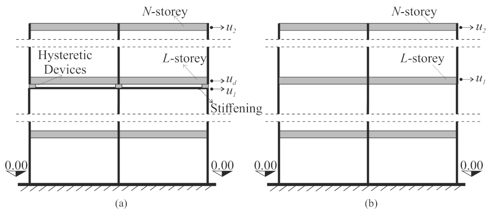
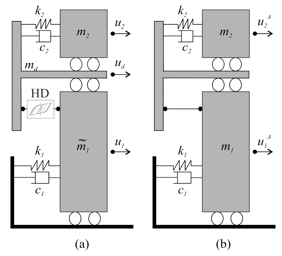
2.1. Archetype Model

In the following, two archetype systems are used to compare results with and without inter-storey isolation. The Main System archetype (MS) represents the structure with the introduction of an intermediate discontinuity (Figure 1a), whereas the Auxiliary System archetype (AS) represents the same structure without the intermediate discontinuity (Figure 1b). In the case of the MS, the part of the structure below the discontinuity is called substructure, whereas the part above the discontinuity is called superstructure.

The MS and AS are 3-DOF and 2-DOF equivalent models, respectively (Figure 2). In such models, $m_1$ and $k_1$ represent the mass and the stiffness of the substructure, whereas $k_2$ and $m_2$ refer to the superstructure. In the MS, the constitutive behaviour of the disconnection devices is modelled by means of the Bouc–Wen model. There are several variations of such a model, for instance, Song and Der Kiureghian [26] proposed a generalized Bouc–Wen model to describe asymmetric hysteresis, whereas Aloisio [27] extended the six-parameters formulation to an eight-parameter formulation to include the cyclical degradation of the material properties. In this paper, the classical Bouc–Wen formulation [28] is deemed fit to accurately describe the constitutive behaviour of the disconnection devices.

It is worth observing that no specific reference is made to any new or existing structures. Moreover, it is assumed that the intermediate discontinuity keeps the structure to be protected in the elastic field. To evaluate the effectiveness of the intermediate discontinuity, the (linear elastic) displacements provided by the MS are compared with those of the AS.

For the MS, the equations of motion, obtained by a direct approach, are written as

$$\begin{array}{c}{c}_{11}{\dot{u}}_1\left(t\right)+c_{12}\dot{u_d}-F_h\left(t\right)+k_1{u}_1\left(t\right)+m_1{\ddot{u}}_1\left(t\right)=-m_1{a}_g\left(t\right),\end{array}$$

(1a)

$$\begin{array}{c}{c}_{21}\dot{u_1}+c_{22}{\dot{u}}_d\left(t\right)+c_{23}{\dot{u}}_2\left(t\right)+F_h\left(t\right)+k_2\left[u_d\left(t\right)-u_2\left(t\right)\right]+m_d{\ddot{u}}_d\left(t\right)=-m_d{a}_g\left(t\right),\end{array}$$

(1b)

$$\begin{array}{c}{c}_{32}\dot{u_d}\left(t\right)+c_{33}\dot{u_2}\left(t\right)+k_2{u}_2\left(t\right)-k_2{u}_d\left(t\right)+m_2{\ddot{u}}_2\left(t\right)=-m_2{a}_g\left(t\right),\end{array}$$

(1c)

$$\begin{array}{c}\dot{z}\left(t\right)=\left[{\dot{u}}_d\left(t\right)-{\dot{u}}_1\left(t\right)\right]\{\tilde{A}-{\left|z\left(t\right)\right|}^n\{{\beta }_1+{\gamma }_1\mathrm{sgn}\left\{z\left(t\right)\left[{\dot{u}}_d\left(t\right)-\dot{u_1}\left(t\right)\right]\right\}\}\}{u}_y^{-1},\end{array}$$

(1d)

where the restoring force $F_h\left(t\right)$ is defined as

$$F_h\left(t\right)=\mathsf{\Psi }{k}_d(u_d\left(t\right)-u_1\left(t\right))+k_d{u}_y(1-\mathsf{\Psi })z\left(t\right),$$

(2)

$z\left(t\right)$ is a hysteretic variable that describes the post-yielding behaviour, whereas $\tilde{A}$, ${\beta }_1$, n, and ${\gamma }_1$ are the Bouc–Wen parameters defined in [28]. The Bouc–Wen parameters are redundant; therefore, both Charalampakis [29] and Ma et al. [30] suggested assigning specific values to some of them. In details, they suggested using $\tilde{A}=1$, so that $k_{\mathrm{d}}=F_y/u_y$ acquires the meaning of pre-yielding (elastic) stiffness. Additionally, some researchers [29,31] suggested using ${\beta }_1+{\gamma }_1=1$, where ${\beta }_1$ and ${\gamma }_1$ are parameters that control the shape and dimension of the hysteresis cycle. The choice to adopt these two constraints, $\tilde{A}=1$ and ${\beta }_1+{\gamma }_1=1$, provides a physical meaning to $F_y$, $u_y$, and $\mathsf{\Psi }$. Specifically, $F_y$ is the yielding force, $u_y$ is the yielding displacement, and $\mathsf{\Psi }$ is the ratio between post-yielding and pre-yielding (elastic) stiffness. Moreover, the values of the hysteretic dimensionless parameter $z\left(t\right)$ remain inside the range $[-1,1]$. Therefore, in this study, the values adopted for the parameters are $\tilde{A}=1$, ${\beta }_1={\gamma }_1=1/2$, and $n=2$.

The damping coefficients $c_{ij}$ in Equations (1a)–(1c) can be grouped in matrix form as

$$\mathbf{C}=\left(\begin{array}{ccc}{c}_{11}& c_{12}& 0\\ c_{21}& c_{22}& c_{23}\\ 0& c_{32}& c_{33}\end{array}\right),$$

(3)

and Matrix $\mathbf{C}$ is derived by means of the classical Rayleigh formulation where $\mathbf{C}={\alpha }_R\mathbf{M}+$${\beta }_R\mathbf{K}$. In this equation, ${\alpha }_R$ and ${\beta }_R$ are the Rayleigh coefficients, and it is assumed that the modal damping of the first two modes is $\xi =0.05$. The elastic stiffness matrix $\mathbf{K}$ and the mass matrix $\mathbf{M}$ are obtained for $\mathsf{\Psi }=1$.

The equations of motion of the AS are described those of a shear-type 2-DOF model. The mechanical behaviour of both MS and AS are considered elastic and linear because the aim of the proposed protection strategy is to maintain the linear elastic behaviour of the structure to be protected. The linear elastic behaviour of the AS is only considered as a reference for the comparison because the AS would conceivably undergo plastic deformations under severe earthquakes. The proposed analytical model does not account for the P-Delta effects that may arise in the columns of the substructure due to the lateral displacement of the superstructure because such displacement is considered negligible, as in [9,10,11].

2.2. Dynamic Equivalence between Multiple-DOF Systems and Archetype Models

This subsection presents the equivalence procedure used to derive the mechanical characteristics of the AS. Such a procedure was developed mainly for low- and medium-rise frame structures and aims at obtaining the masses $m_1$ and $m_2$ and stiffnesses $k_1$ and $k_2$ of the AS starting from the geometrical and mechanical characteristics of the multiple-DOF (M-DOF) frame structure without intermediate discontinuity. If the response of the M-DOF frame has a predominant vibration mode, then the AS can correctly represent the behaviour of such a M-DOF system. The equivalence procedure is described in the details in [21]. It is assumed that $m_1$, $m_2$, $k_1$, and $k_2$ remain the same for the MS. The procedure is based on the following two assumptions:

• The frequency ${\omega }_m$ of the main mode of the M-DOF system without discontinuity and of the first mode of the AS (Figure 2b) are the same;
• The modal displacements of the storey of the discontinuity and top storey (i.e., L-th and N-th storeys in Figure 1a of the M-DOF system without discontinuity are equal to the modal displacements $u_1$ and $u_2$ of the AS.

The masses $m_1$ and $m_2$ of the AS correspond to the total mass of the substructure and superstructure, respectively. Assuming storeys of equal mass m entails

$$m_1=mL;m_2=m(N-L),$$

(4)

where m is the mass of a storey, L is the level where the intermediate discontinuity is introduced, and N is the number of storeys of the frame. The masses of the MS are ${\tilde{m}}_1$, $m_d$, and $m_2$. In particular, the mass of the substructure reads

$${\tilde{m}}_1=m(L-1)+m_0;m_d=m,$$

(5)

where $m_0=\gamma m$ ($\gamma =0.5$) is the mass of additional stiffening elements. Such stiffening elements are those that should be added to the level just below the discontinuity to maintain the same lateral stiffness available before the introduction of the discontinuity (Figure 1a). The value $\gamma =0.5$ is chosen because only horizontal structural elements are needed to restore the stiffness of the disconnected storey, which, consequently, has a mass smaller than that of an entire storey.

The equivalence procedure requires the identification of the main mode of the M-DOF frame structure without discontinuity. It is assumed that the main mode of the structure has the highest modal mass participation factor $\mathcal{L}$. Let $\mathsf{\Phi }$ be the vector that collects the modal displacements along a reference vertical line and along the direction to which corresponds the highest factor $\mathcal{L}$. It reads

$$\mathrm{\Phi }={\left\{{\varphi }_1,{\varphi }_2,\dots ,{\varphi }_L,\dots ,{\varphi }_{N-1},{\varphi }_N\right\}}^T$$

(6)

The following relationships for equivalent stiffnesses $k_1$ and $k_2$ of the AS can be obtained as in [21]:

$$k_1=\frac{{\omega }_m^2(m_1{\varphi }_L+m_2{\varphi }_N)}{{\varphi }_L};k_2=\frac{{\omega }_m^2{m}_2{\varphi }_N}{{\varphi }_N-{\varphi }_L},$$

(7)

where ${\varphi }_L$ and ${\varphi }_N$ are the components of the vector $\mathsf{\Phi }$ that refer to the L and N storeys of the M-DOF system.

It is worth remarking that the stiffness values of the superstructure and substructure are assumed to remain unchanged after the discontinuity is introduced (i.e., $k_1$ and $k_2$ obtained by Equation (7) are the same for both AS and MS). The ability of both MS and AS to describe a generic 3D frame structure, without and with intermediate discontinuity, and the limitations of such archetype models were discussed in [23].

2.3. Characteristics of the Frame

The reference building is a regular six-storeys frame structure. The storey mass is $m_p=301.5$ kg $\times {10}^3$, that correspond to a storey area of 300 m${}^2$. The viscous damping ratio of the frame structure is $\xi =5\%$ and the overall storey stiffness is $k_p=476,779\mathrm{KN}/\mathrm{m}$. The fundamental period of such a structure is $T=0.65$ s. For a six-storey building, the intermediate discontinuity can be placed at five different levels. The characteristics of the archetype models depend on the discontinuity level L and are reported in

Table 1. Mechanical characteristics of MS and AS archetypes.

L	${\mathit{m}}_1$ [kg $\times {10}^3$]	$\widetilde{{\mathit{m}}_1}$ [kg $\times {10}^3$]	${\mathit{m}}_2$ [kg $\times {10}^3$]	${\mathit{k}}_1$ [kN/m]	${\mathit{k}}_2$ [kN/m]
1	301.5	150.75	1507.50	602,403	182,552
2	603.0	425.25	1206.00	292,175	208,839
3	904.5	735.75	904.50	207,567	250,374
4	1206	1055.25	603.00	177,681	324,132
5	1507.5	1356.75	301.50	167,962	476,779

.

2.4. Gain Coefficients

The results of the MS are compared with those of the AS to verify if the introduction of the intermediate discontinuity reduces the displacements and drifts of the structure. The comparison between the displacements and drifts of the two models is made through three coefficients that are named gain coefficients and are defined as

$${\alpha }_1=\frac{\max \left[u_1\left(t\right)\right]}{\max \left[u_1^A\left(t\right)\right]};{\alpha }_2=\frac{max[u_2\left(t\right)-u_d\left(t\right)]}{max[u_2^A\left(t\right)-u_1^A\left(t\right)]};{\alpha }_3=\frac{\max [u_d\left(t\right)-u_1\left(t\right)]}{u_0},$$

(8)

where the displacements $u_1$, $u_2$, and $u_d$ refer to the MS (Figure 2a), $u_1^A$ and $u_2^A$ refer to the AS (Figure 2b), and $u_0$ is the threshold value of the acceptable displacements. The proposed gain coefficients represent a relative evaluation of the effectiveness of the hysteretic intermediate discontinuity. They evaluate the performances of the system with the discontinuity with respect to a reference system, represented by the corresponding linear elastic system without intermediate discontinuity.

The gain coefficient ${\alpha }_1$ refers to the substructure and is the ratio between the displacements of the substructures of the MS and AS. Such a coefficient evaluates the performance of the superstructure as TMD for the substructure. The gain coefficient ${\alpha }_2$ refers to the superstructure and is the ratio between the drifts of the superstructure of the MS and AS. In this case, ${\alpha }_2$ evaluates the behaviour of the intermediate discontinuity as base isolation for the superstructure. Finally, ${\alpha }_3$ is the ratio between the displacement of the intermediate discontinuity and the maximum threshold value $u_0=15$ cm. Such value was chosen in order to limit excessive displacements on the discontinuity layer that may jeopardize the safety of the structure. Each gain coefficient evaluates a different capability of the intermediate discontinuity. If a gain coefficient is less than unity, the introduction of the discontinuity is beneficial for a specific part of the structure. Therefore, the improvement of the dynamical behaviour of the frame means obtaining gain coefficients lower than unity (i.e., a reduction of displacements and drifts). A simultaneous control on these coefficients leads to a unitary approach to the dynamic enhancement of the structure following from the introduction of the discontinuity.

Two additional gain coefficients are introduced with the purpose to evaluate how the intermediate discontinuity affects the accelerations of the substructure and superstructure. They read

$${\alpha }_1^A=\frac{\max \left[{\ddot{u}}_1\left(t\right)\right]}{\max \left[{\ddot{u}}_1^A\left(t\right)\right]};{\alpha }_2^A=\frac{max[{\ddot{u}}_2\left(t\right)-{\ddot{u}}_d\left(t\right)]}{max[{\ddot{u}}_2^A\left(t\right)-{\ddot{u}}_1^A\left(t\right)]},$$

(9)

where ${\ddot{u}}_1\left(t\right)$, ${\ddot{u}}_2\left(t\right)$, and ${\ddot{u}}_d\left(t\right)$ are the accelerations of the MS. Similarly, ${\ddot{u}}_2^A\left(t\right)$ and ${\ddot{u}}_1^A\left(t\right)$ are the accelerations of the AS.

2.5. Variable Parameters

The parametric analysis is performed by varying the following parameters:

• Post-yielding to pre-yielding stiffness ratio $\mathrm{\Psi }$.
• Yield displacement ratio $\eta =\frac{u_y}{u_0}$.
• Pre-yielding to storey stiffness ratio $\rho =\frac{k_d}{k_p}$.
• Ratio between $m_2$ (Equation (4)) and ${\tilde{m}}_1$ (Equation (5)) $\mu =\frac{m_2}{{\tilde{m}}_1}$.
• Discontinuity level of the frame structure L.

The results presented in the following sections are obtained by numerically integrating the equations of motion. For this purpose, an original code is developed in the Mathematica® software. The equations of motion are integrated in an implicit form and the adopted step size is $\delta t=0.01$ s.

3. Harmonic Analysis

The harmonic analyses are conducted on the frame whose characteristics are reported in Table 1. Parametric analyses are carried out to identify how the parameters influence the response of the system with the discontinuity. In the analyses, the external excitation is defined as

$$a_g\left(t\right)=A\mathrm{Sin}\left(\mathsf{\Omega }t\right),$$

(10)

with A amplitude and $\mathsf{\Omega }$ circular frequency of the excitation. Since the system is non-linear, A is considered as a variable parameter.

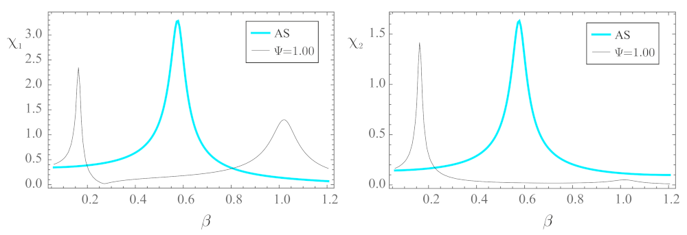
3.1. Frequency-Response Curves

A first analysis compares the frequency-response curves of the MS and AS. Such curves represent the dimensionless maximum displacement of the substructure, ${\chi }_1=$$\mathrm{Max}\left(\right|u_1\left(t\right)|/u_0$), and the dimensionless drift of the superstructure, ${\chi }_2=$$\mathrm{Max}\left(\right|u_2\left(t\right)-u_d\left(t\right)|/u_0$), as functions of the frequency ratio $\beta =\mathsf{\Omega }/{\omega }_1$, where ${\omega }_1=\sqrt{k_1/m_1}$. In the analyses where the value of $\eta$ is fixed, such value is assumed as $\eta =0.2$.

Figure 3 compares the frequency-response curves of the MS obtained for $\mathrm{\Psi }$ = 1.0, and the frequency-response curves of the AS. Assuming $\mathrm{\Psi }$ = 1.0 entails a linear behaviour of the discontinuity, the comparison shows that the discontinuity introduces a second peak in the frequency-response curves of the MS. Such a peak corresponds to a second resonant frequency, whereas the AS is characterized by a single resonant frequency in the range of the observed frequencies. The existence of a second resonant frequency is a consequence of the presence of a TMD in the system, meaning that, due to the discontinuity, the superstructure works as a TMD for the substructure. The frequency-response curve of ${\chi }_2$ shows a shift of the main frequency of the MS to lower values and highlights a behaviour as a base isolated structure. Thus, the superstructure acts as a TMD for the substructure and the superstructure behaves as if it was base-isolated. In both cases, it can be asserted that the distance between the two resonant frequencies of the MS is a qualitative measure of the effectiveness of the discontinuity.

A second analysis investigates the sensitivity of the system to the values of the parameters characterizing the hysteretic behaviour of the disconnection devices. Figure 4 shows the frequency-response curves obtained for several values of the parameters characterizing the Bouc–Wen constitutive law. Specifically, Figure 4a shows the frequency-response curves of the MS for $L=3$, $A=0.6$ g, $\rho =0.2$, and several values of $\mathrm{\Psi }$ increasing from $\mathrm{\Psi }=0.10$ to $\mathrm{\Psi }=1.00$. The highest resonant frequency is not significantly sensitive to $\mathrm{\Psi }$; on the contrary, the smallest resonant frequency significantly depends on $\mathrm{\Psi }$. The values of both ${\chi }_1$ and ${\chi }_2$ in correspondence of the resonant peaks strongly depend on $\mathrm{\Psi }$. As $\mathrm{\Psi }$ decreases, the hysteresis cycles become larger, and the values of the dimensionless displacements in correspondence of the peak decrease. Moreover, the distance between the peaks increases as $\mathrm{\Psi }$ decreases. Figure 4b shows the frequency-response curves for $L=5$, $A=0.6$ g, $\rho =0.2$, and the same values of $\mathrm{\Psi }$ of the case presented in Figure 4a. When the discontinuity is placed at higher levels, the values of ${\chi }_1$ and ${\chi }_2$ at the resonant peak that refers to the lower frequency reduce as $\mathrm{\Psi }$ decreases. The value of $\mu$ obtained for $L=5$ is smaller than the value obtained for $L=3$, and the distance between the two resonant peaks decreases, thus reducing the frequency range where the discontinuity is effective. Figure 4c shows the frequency-response curves obtained for different values of $\rho$ increasing from $\rho =0.02$ to $\rho =0.30$, $L=3$, $A=0.6$ g, and $\mathrm{\Psi }=0.25$. As $\rho$ increases, both the first and second resonant frequencies shift toward higher values. Moreover, ${\chi }_1$ manifests higher values at the resonant peaks for smaller values of $\rho$. The same increase occurs for the values at the left peak of the ${\chi }_2$ curves. Instead, the value of ${\chi }_2$ at the higher resonant frequency decreases until it almost vanishes for decreasing values of $\rho$, thus confirming that, for small values of $\rho$, the discontinuity acts on the superstructure as a base isolation. The last sub-figure, Figure 4d, shows the frequency-response curves referring to the MS that are obtained for different values of A and assuming $L=3$, $\mathrm{\Psi }=0.25$, and $\rho =0.2$. For increasing values of A the position of the peaks slightly shifts leftwards on the $\beta$-axis (i.e., the two resonant frequencies are only slightly sensitive to the value of A).

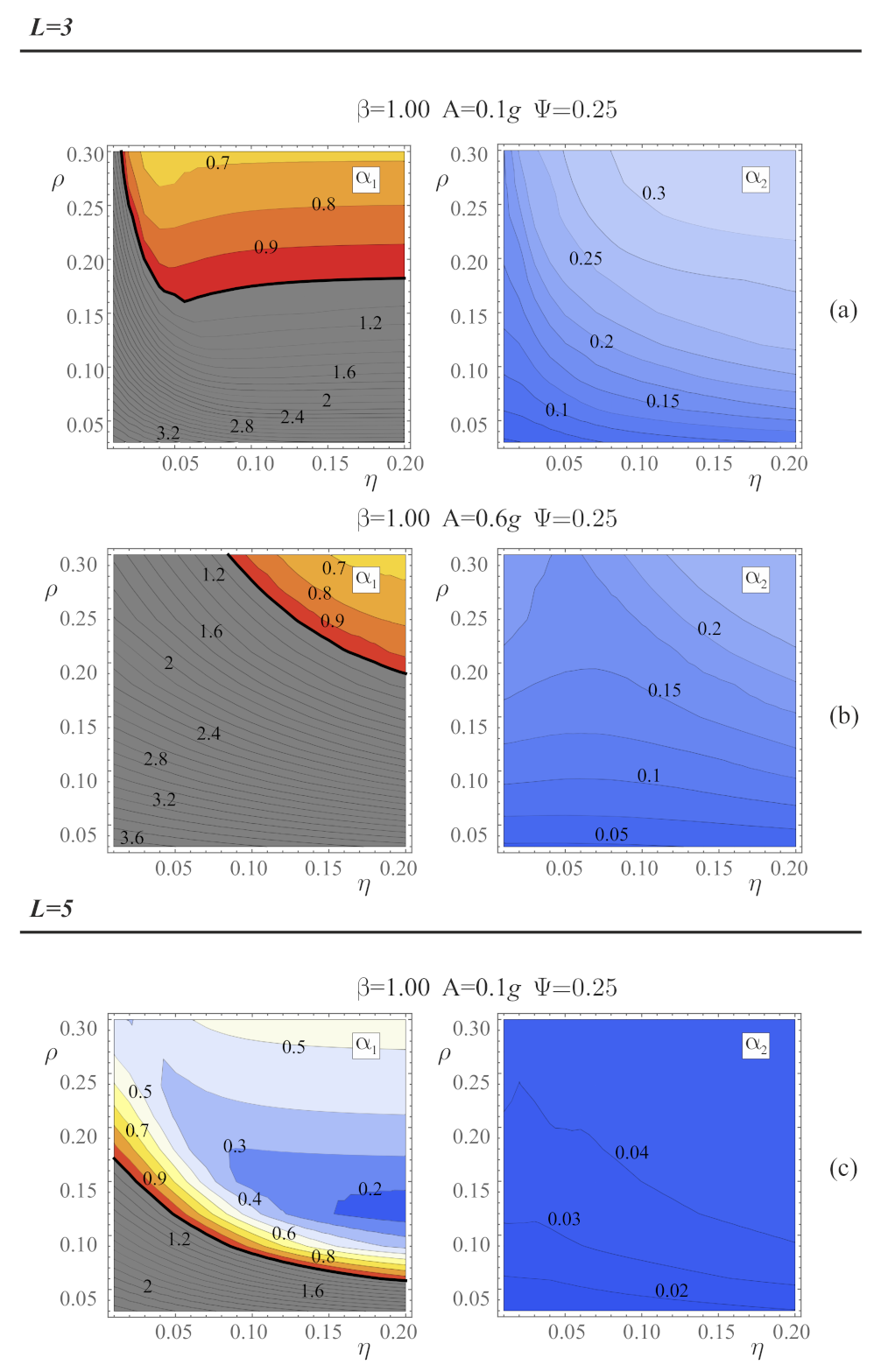
3.2. Gain Maps

This section analyses how $\mathrm{\Psi }$ affects the dynamical behaviour of the system with intermediate discontinuity. The effects of increasing values of $\mathrm{\Psi }$ are assessed by evaluating the gain coefficient Equations (8) and (9). The results of the parametric analysis are summarised in gain maps that represent the gain coefficients, ${\alpha }_1$ and ${\alpha }_2$, plotted in the parameter plane $\eta -\rho$. Each map refers to a specific value of $\mathrm{\Psi }$. The maps on the left column of Figure 5 are obtained for $\mathrm{\Psi }=0.25$, whereas the maps on the right column refer to $\mathrm{\Psi }=0.75$. Moreover, the maps of Figure 5a show the ${\alpha }_1$ coefficient, whereas the maps of Figure 5b show the ${\alpha }_2$ coefficient. The maps are obtained for $\beta =0.75$ and $A=0.1$ g; they show a strong dependence on $\rho$ and, up to a threshold value, on $\eta$. At higher values of $\eta$ (where the value of $\eta$ depends on the considered map), the gain coefficients become independent of $\eta$ (i.e., in both the ${\alpha }_1$ and ${\alpha }_2$ maps, the contour levels tend to become horizontal). It is useful to remark that $\eta$ directly depends on the yielding displacement; hence, high values of $\eta$ refer to high values of $u_y$. A frame with intermediate discontinuity and small values of $\eta$ manifests a stronger non-linear behaviour of the disconnection devices than systems with higher $\eta$. For very high value of $\eta$, the disconnection devices tend to manifest a linear elastic behaviour since the high-yielding displacement $u_y$ cannot be reached during the motion. The impossibility to reach $u_y$ during the motion is more evident at higher values of the stiffness ratio $\mathrm{\Psi }$, due to the higher post-elastic stiffness of the disconnection devices. For the chosen values of $\beta$, A, and $\mathrm{\Psi }$, both ${\alpha }_1$ and ${\alpha }_2$ are smaller than unity in the whole parameter plane, which means that the intermediate discontinuity reduces the displacement of the substructure and the drift of the superstructure with respect to those of the original frame structure.

Under a harmonic excitation, after a transient time that depends on the damping of the structure, the system undergoes stationary dynamics. To understand the behaviour of the disconnection devices for increasing values of $\eta$, the stationary hysteretic cycles are shown for points ${\mathrm{P}}_1$ and ${\mathrm{P}}_3$ in Figure 5c, and for points ${\mathrm{P}}_2$ and ${\mathrm{P}}_4$ in Figure 5d. The hysteretic cycles show the value of the dimensionless force ${\sigma }_h=F_h/k_d{u}_y$ as a function of the dimensionless displacement ${\chi }_d=u_d\left(t\right)/u_y$. By comparing the cycles in the first column of Figure 5c,d, which refer to $\mathrm{\Psi }=0.25$, with the cycles in the second column, which are obtained for $\mathrm{\Psi }=0.75$, it can be observed that a higher value of $\mathrm{\Psi }$ corresponds to smaller hysteresis cycles. Similarly, an increase of $\eta$ also leads to a reduction of the area of the hysteretic cycles (compare the cycles of Figure 5c,d).

Figure 6 shows the gain maps obtained for $\beta =1$ and $\mathrm{\Psi }=0.25$. The maps in Figure 6a and Figure 6b are obtained for $A=0.1$ g and $A=0.6$ g, respectively, assuming that the discontinuity is located at the third level ($L=3$). Figure 6c, instead, shows maps obtained for $A=0.1$ g and a discontinuity located at the fifth level ($L=5$). The comparison of Figure 6a and Figure 6b highlights the dependence of the gain maps on A. Specifically, in the gain maps of Figure 6b, the contour levels do not tend to a horizontal asymptote because the displacement of the disconnection devices exceeds the yield displacement $u_y$ due to the high value of A, thus assuring wide hysteresis cycles.

The ${\alpha }_1$ gain maps of Figure 6a,b show that there are large regions of the parameter where the gain coefficients are higher than unity (dark grey regions). In these regions, the discontinuity is not able to reduce the displacement of the substructure. On the contrary, ${\alpha }_2$ is smaller than unity in the whole parameter plane, thus assuring a reduction of the superstructure drift for any combination of the parameters. Nevertheless, it is always possible to choose a combination of the design parameters $\rho$ and $\eta$ inside regions where both the gain coefficients ${\alpha }_1$ and ${\alpha }_2$ are smaller than unity.

The comparison among the left maps of Figure 5a,b and the maps of Figure 6a (all obtained for $\mathrm{\Psi }=0.25$ and $A=0.1$ g) shows that the effectiveness of the discontinuity (i.e., the smallness of the gain coefficients) strongly depends on the frequency ratio $\beta$.

Finally, Figure 6c shows the gain maps for $L=5$. In this case, the dark grey regions where ${\alpha }_1$ is higher than unity reduce compared to the case with $L=3$, and, generally, smaller values of both ${\alpha }_1$ and ${\alpha }_2$ are obtained, thus showing the higher effectiveness of the intermediate discontinuity.

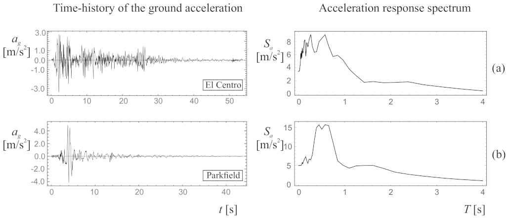
4. Seismic Analysis

This section shows the results of a seismic analysis. The first part of the section aims at providing an initial understanding of the seismic behaviour of the MS. For this purpose, the gain maps show the results of simulations performed using single seismic records as excitation. The two different seismic records considered in this analysis are:

(a)

El Centro, CA, Array Station 9, Imperial Valley Irrigation District, component 180;

(b)

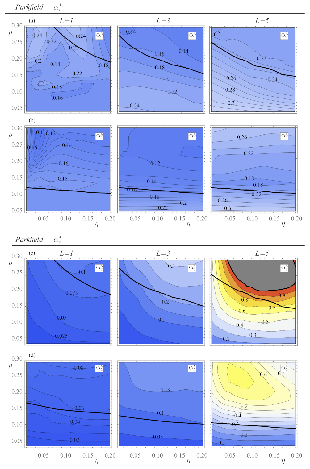
Parkfield, CO2-065 ground motion recorded during the California earthquake 1966.

Figure 7 shows the time-histories (left graphs) and the pseudo-response spectra (right graphs) of the two seismic records. In the following, each seismic record is called with the corresponding earthquake name (i.e., the names underlined in the list above).

Since gain maps referred to a single registration are not useful for a complete assessment of the effectiveness of the intermediate discontinuity, the second part of the section shows the results of an analysis carried out considering $n_e=305$ seismic records. The complete list of seismic records used in the analysis can be found at http://ing.univaq.it/diegidio/Earthq/Earthquakes_Table.pdf. Additionally, in this case, the results are presented in gain maps. Such gain maps show the mean values of the gain indexes obtained with the different seismic records.

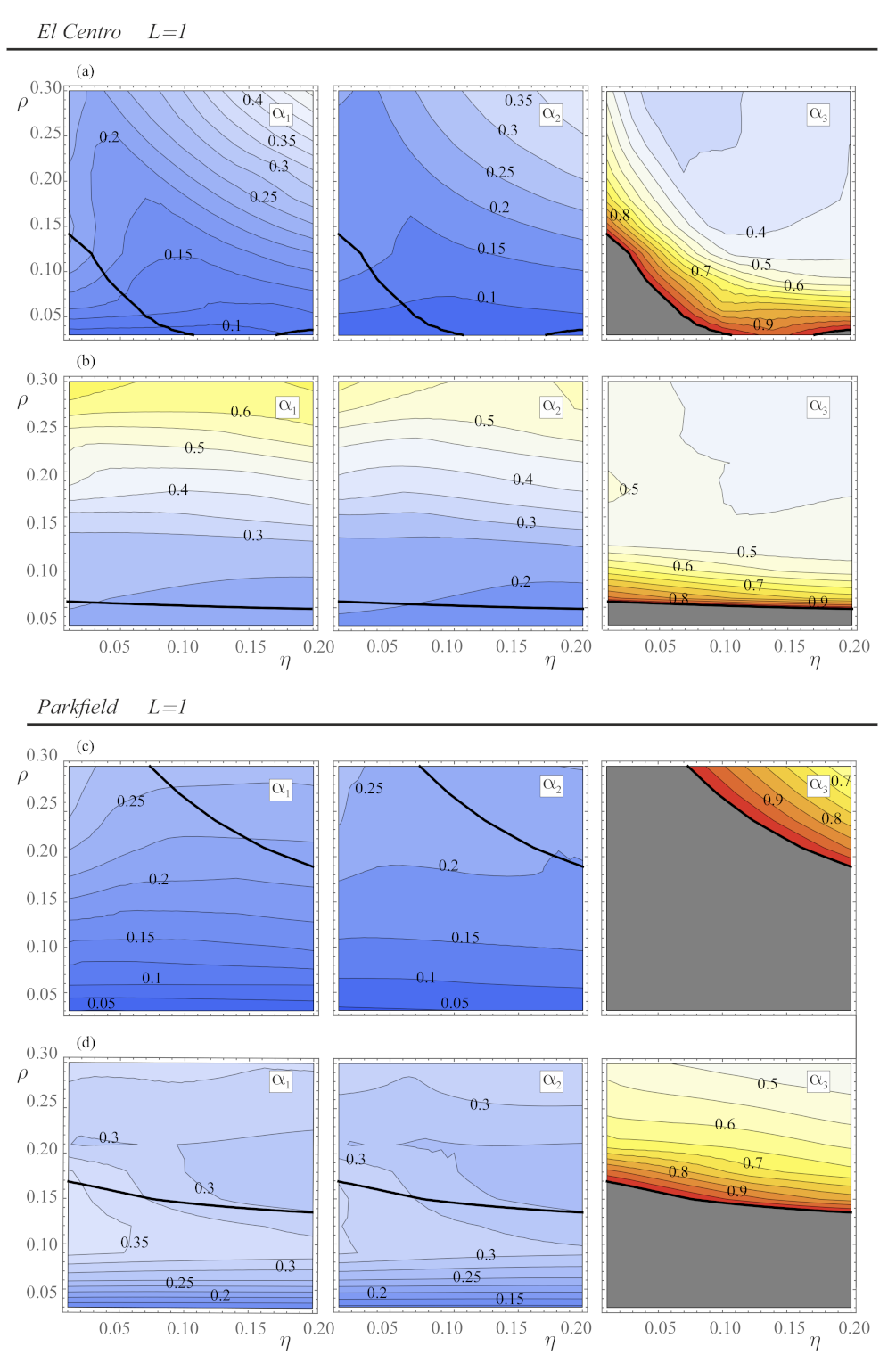
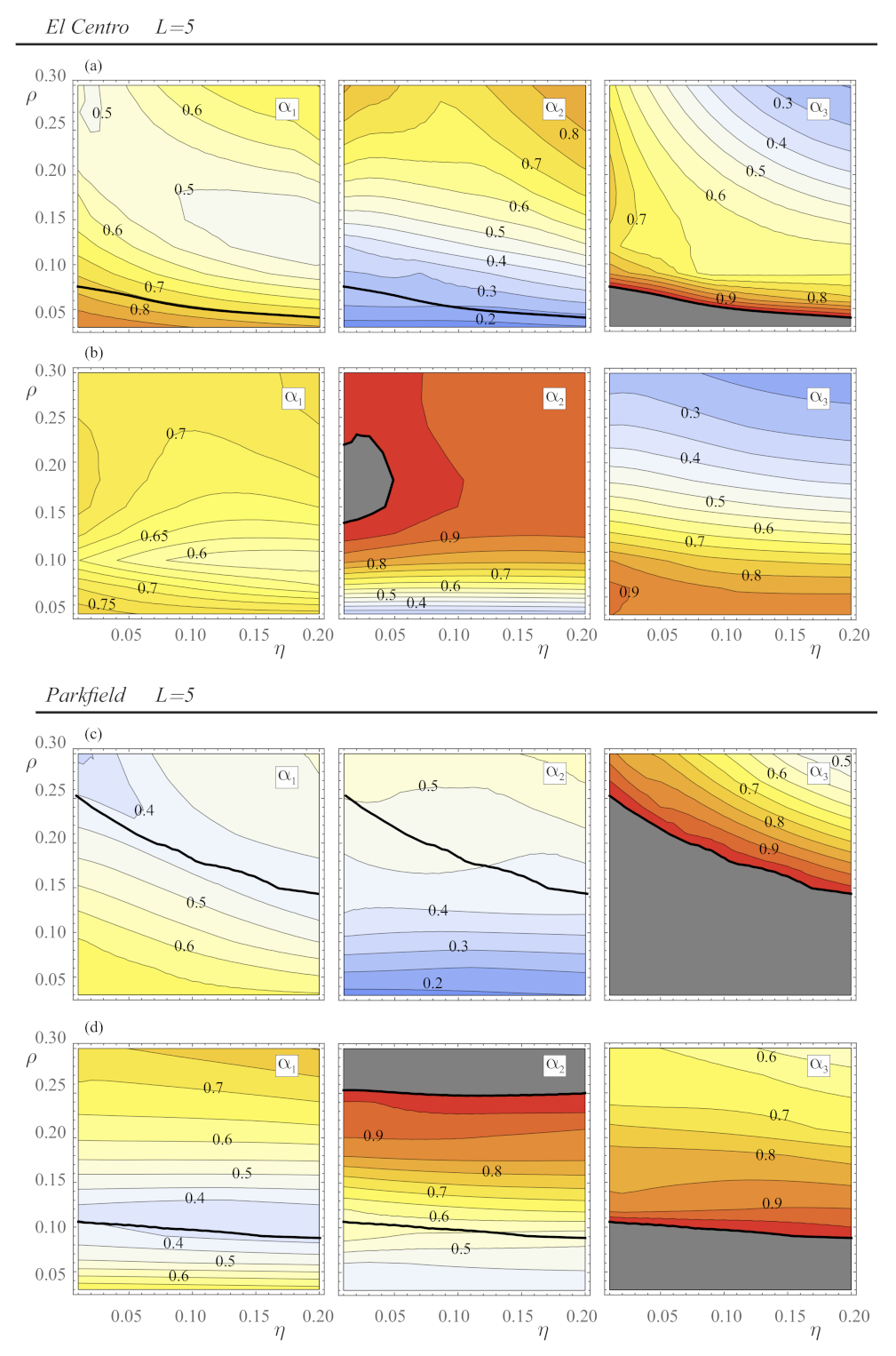
4.1. Gain Maps from a Single Seismic Record

Figure 8, Figure 9 and Figure 10 show the gain maps obtained with the seismic records of El Centro and Parkfield for $L=1$, $L=3$, and $L=5$, respectively. Specifically Figure 8a–c, Figure 9a–c and Figure 10a–c are obtained for $\mathrm{\Psi }=0.25$, whereas Figure 8b–d, Figure 9b–d, and Figure 10b–d for $\mathrm{\Psi }=0.75$. The regions where the gain coefficients ${\alpha }_1$ and ${\alpha }_2$ are smaller than unity are coloured, those where these gain coefficients are higher than unity are displayed in dark grey colour. Both the ${\alpha }_1$ and ${\alpha }_2$ maps show that, as $\mathrm{\Psi }$ increases, the gain coefficients increase, thus reducing the effectiveness of the intermediate discontinuity. The ${\alpha }_3$ maps show the feasibility of the protection strategy. When ${\alpha }_3$ is higher than unity (dark grey zones of the ${\alpha }_3$ maps), the displacements of the disconnection devices are higher than the permissible threshold value. The size of the dark grey zones in the ${\alpha }_3$ maps increases when $\mathrm{\Psi }$ decreases, thus even if lower values of $\mathrm{\Psi }$ assure a higher reduction of displacements and drifts, the displacements of the discontinuity level may not be compatible with the capability of the disconnection devices.

In Figure 8, Figure 9 and Figure 10, the thick black lines on the maps represent the admissible limit of ${\alpha }_3$. In each map, only in the region above such lines, the displacement of the discontinuity is below the threshold value $u_0$. While the ${\alpha }_3$ gain maps obtained from the seismic record of El Centro show only small dark grey regions, the ${\alpha }_3$ gain maps obtained from the Parkfield seismic record show large regions where ${\alpha }_3>1$ maps. The size of these regions significantly reduces as $\mathrm{\Psi }$ increases. Moreover, when the discontinuity level L increases, the size of the dark grey regions tends to reduce.

Figure 11 and Figure 12 show the ${\alpha }_1^A$ and ${\alpha }_2^A$ gain maps under El Centro and Parkfield seismic records, respectively. These maps evaluate the effects of the discontinuity on the accelerations of the structure. The black lines on the maps show the range highlighted in the ${\alpha }_3$ maps of Figure 8, Figure 9 and Figure 10. Only in the regions above such lines are the displacements of the disconnection devices below the admissible threshold. In Figure 11 and Figure 12, the maps in the first two rows refer to ${\alpha }_1^A$, whereas the maps in the third and fourth rows refer to ${\alpha }_2^A$. The maps in the first and third rows are obtained for $\mathrm{\Psi }=0.25$, the maps in the second and fourth rows refer to $\mathrm{\Psi }=0.75$.

The ${\alpha }_1^A$ maps show that as $\mathrm{\Psi }$ increases, ${\alpha }_1^A$ decreases. Similarly, ${\alpha }_2^A$ decreases as $\mathrm{\Psi }$ increases. Therefore, a lower value of $\mathrm{\Psi }$ may increase the accelerations and, at the same time, reduce displacements and drifts. However, both the gain coefficients based on the displacements and drifts (Equation (8)) and those based on the accelerations (Equation (9)) are smaller than unity in a large area of the parameters plane. It is worth observing that ${\alpha }_1^A$ and ${\alpha }_2^A$ are lower than ${\alpha }_1$ and ${\alpha }_2$, thus the use of ${\alpha }_1$ and ${\alpha }_2$ provides a more severe assessment of the effectiveness of the intermediate discontinuity.

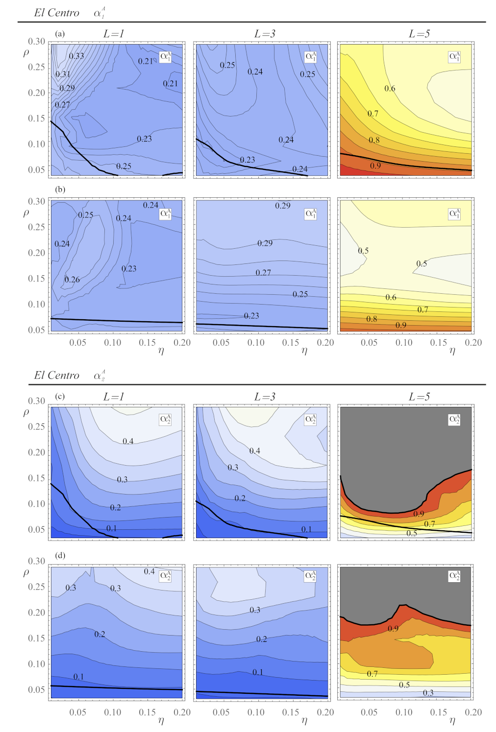
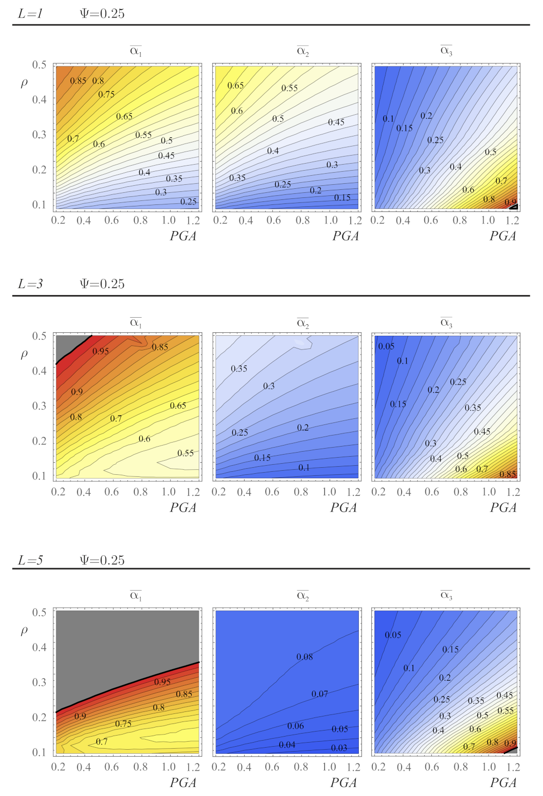
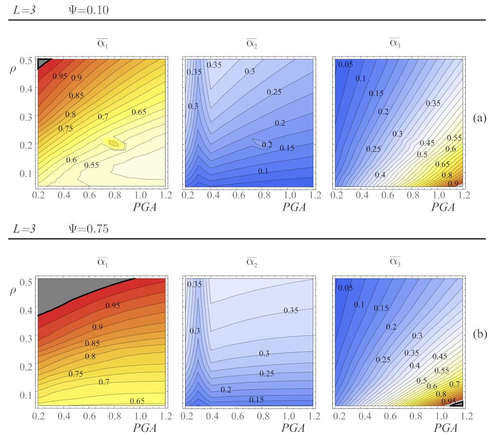
4.2. Gain Maps Obtained from Multiple Seismic Records

The seismic analysis is carried out by using several seismic records obtained from [32]. The magnitude varies from 4 to 8 and the epicentral distance varies from 10 to 30 km. In the analysis, the target parameters are the mean displacements ${\overline{u}}_i$ that are defined as the mean of the maximum displacements $u_{i,j}$ obtained from the integration of the equations of motion with each seismic record; they read

$${\overline{u}}_i=\frac{1}{n_e}\sum _{j=1}^{n_e}max\left[u_{i,j}\left(t\right)\right]$$

(11)

with $(i=1,d,2)$. The displacements $u_{1,j}$, $u_{d,j}$, and $u_{2,j}$ are those of the substructure, discontinuity level, and superstructure obtained from the jth seismic record. The total number of seismic records used in the simulations is $n_e$. The number of seismic records used is sufficient to reach a coefficient of variation (CoV) of ${\overline{u}}_i$, CoV${}_{{\overline{u}}_i}\le 0.2$. Therefore, the predictability of the model to identify the average displacement is higher than 80%. The CoV${}_{{\overline{u}}_i}$ is defined as

$$Co{V}_{{\overline{u}}_i}=\frac{\sigma \left({\overline{u}}_i\right)}{\mu \left({\overline{u}}_i\right)}$$

(12)

where $\sigma \left({\overline{u}}_i\right)$ and $\mu \left({\overline{u}}_i\right)$ are the standard deviation and mean value of ${\overline{u}}_i$, respectively. To understand the effectiveness of the disconnection, three coefficients (called mean-gain coefficients in the following) similar to those in Equation (8) are introduced:

$$\overline{{\alpha }_1}=\frac{{\displaystyle \sum _{j=1}^{n_e}}\max \left[u_{1,j}\left(t\right)\right]}{{\displaystyle \sum _{j=1}^{n_e}}\max \left[u_{1,j}^A\left(t\right)\right]};\overline{{\alpha }_2}=\frac{{\displaystyle \sum _{j=1}^{n_e}}\max [u_{2,j}\left(t\right)-u_{d,j}\left(t\right)]}{{\displaystyle \sum _{j=1}^{n_e}}\max [u_{2,j}^A\left(t\right)-u_{1,j}^A\left(t\right)]};\overline{{\alpha }_3}=\frac{{\displaystyle \sum _{j=1}^{n_e}}\max [u_{d,j}\left(t\right)-u_{1,j}\left(t\right)]}{n_e{u}_0}$$

(13)

Figure 13 shows the gain maps of the mean displacements. Such maps represent the mean-gain coefficients in the parameters plane $PGA$-$\rho$, where $PGA$ is the peak ground acceleration and $\rho$ is the stiffness ratio previously defined. All the gain maps are obtained for $\eta =0.2$. Similarly to previous figures, the regions where ${\overline{\alpha }}_i<1,(i=1,2)$ are named gain regions and are coloured, whereas those where ${\overline{\alpha }}_i>1$ are identified by a dark grey colour. The first, second, and third rows of the figure refer to different levels of the discontinuity, $L=1$, $L=3$, and $L=5$, respectively. All maps are obtained for $\mathrm{\Psi }=0.25$.

The maps show wide gain regions. As can be observed, $L=1$ provides the best performances in the reduction of the displacement of the substructure because the values of ${\overline{\alpha }}_1$ obtained for $L=1$ are in general smaller than those obtained for other values of L. On the contrary, $L=5$ provides the largest reduction of the drift of the superstructure since, in this case, ${\overline{\alpha }}_2$ is smaller than those in the other cases. The maps of ${\overline{\alpha }}_3$ show values higher than unity only in the zone with high values of $PGA$ and low values of $\rho$, specifically in the region where $PGA>1.1$ g and $\rho <0.1$. In this region, ${\overline{\alpha }}_1$ and ${\overline{\alpha }}_2$ have small values, but the displacement of the discontinuity level exceeds the threshold value $u_o$ (i.e., ${\overline{\alpha }}_3$ is higher than unity). Nevertheless, such a region is very small and a slight increase of $\rho$ is sufficient to move in a region of the maps where ${\overline{\alpha }}_3\le 1$ and at the same ${\overline{\alpha }}_1\le 1$ and ${\overline{\alpha }}_2\le 1$. Since all the three coefficients are less than unity the disconnection can be considered a successful protection strategy for the original frame structure. The map obtained for $L=3$ shows an intermediate behaviour between those obtained for $L=1$ and $L=5$, and the map of ${\overline{\alpha }}_3$ does not show any dark grey regions.

To summarize, the ${\overline{\alpha }}_1$ maps exhibit a decrease in the performance from $L=1$ to $L=5$. This can be explained by assuming that the superstructure acts as a TMD for the substructure and consequently the performance decreases because the mass ratio between the superstructure and substructure decreases [7,22]. Instead, ${\overline{\alpha }}_2$ decreases from $L=1$ to $L=5$. In this case, when $L=5$, the superstructure is very stiff and the superstructure acts as if it was base-isolated. On the contrary, when $L=1$, the superstructure has lower stiffness and the performance decreases since the period of the superstructure can approach that of the discontinuity layer. Similar results were already presented in [33] for tower buildings.

Figure 14 shows the mean-gain maps obtained for $L=3$. The maps in the first row refer to $\mathrm{\Psi }=0.1$, whereas the maps in the second row are obtained for $\mathrm{\Psi }=0.75$. A direct comparison with the maps in the second row of Figure 13 ($L=3$) allows evaluating the effect of $\mathrm{\Psi }$ on the performances of the intermediate discontinuity. The dark grey region of the ${\overline{\alpha }}_1$ map enlarges with respect to that of Figure 13 for increasing $\mathrm{\Psi }$. Therefore, lower values of $\mathrm{\Psi }$ allow a wider range of use. Moreover, when $\mathrm{\Psi }$ decreases, the performance of the system increases since there is a higher reduction of the displacement of the substructure (i.e., a decrease of ${\alpha }_1$). On the contrary, the coefficients ${\overline{\alpha }}_2$ and ${\overline{\alpha }}_3$ are not significantly affected by $\mathrm{\Psi }$. Finally, ${\overline{\alpha }}_3$ is always smaller than unity when $\mathrm{\Psi }<0.25$, whereas for $\mathrm{\Psi }=0.75$ there is a small region where ${\overline{\alpha }}_3\ge 1$.

5. Conclusions

This paper proposes a modelling approach for the study of the intermediate discontinuity. The structure with the discontinuity layer has been modelled by a 3-DOF model and the disconnection devices have been described by using the Bouc–Wen model. In order to evaluate the improvement of the dynamical behaviour obtained by the introduction of the discontinuity, two different systems have been analysed. The first system is the frame after the introduction of the discontinuity, called the main system (MS) and the second system is the reference frame, called the auxiliary system (AS).

The first part of the paper is focused on the dynamical behaviour of the MS that is analysed by using harmonic excitation. The results of the analysis have been organized in frequency-response curves and gain maps. It has been found that the value of the post-yielding to pre-yielding stiffness ratio $\mathrm{\Psi }$ in the Bouc–Wen model significantly affects the value of the first frequency of the MS. Moreover, by comparing the frequency-response curves of the AS and MS for different values of $\mathrm{\Psi }$, it has been found that lower values of $\mathrm{\Psi }$ may extend the range of frequency where the intermediate discontinuity is effective. The harmonic maps highlighted that small values of $\mathrm{\Psi }$ may reduce the displacement of the superstructure, but also increase the displacement of the substructure.

The second part of the paper is focused on the seismic response of the models. A preliminary analysis has been carried out considering single seismic records. Five gain coefficients have been defined to evaluate the effects of the introduction of the intermediate discontinuity. Such coefficients have been defined as ratios between the displacements (or the accelerations) of the MS and those of the AS. The results of the analysis have been summarized in gain maps. Such maps show the gain coefficients in a specific parameters plane. The results also show that an increase of $\mathrm{\Psi }$ reduces the displacement of the substructure and increases that of the superstructure. Moreover, higher values of $\mathrm{\Psi }$ reduce the displacement of the discontinuity layer, thus reducing the likelihood of such displacement exceeding a threshold value. It has been found that another possibility to reduce the displacement of the discontinuity layer is to change the level of the discontinuity L. As L increases, the displacement of the discontinuity layer decreases due to the filtering effect of the substructure. Additionally, the effects of the intermediate discontinuity on the accelerations acting on the structure have been evaluated, and it has been found that when $\mathrm{\Psi }$ decreases, the accelerations may increase.

Finally, a seismic analysis is carried out considering several seismic records within definite ranges of magnitude and epicentral distance. The results have been organized in gain maps that show the gain coefficients in different parameters planes. Such maps may be a useful auxiliary tool in the understanding of the behaviour resulting from the introduction of an intermediate discontinuity in a frame structure.

References

- Kelly, J. Base isolation: Linear theory and design. Earthq. Spectra 1995, 6, 223–244. [Google Scholar] [CrossRef]
- Den Hartog, J.P. Mechanical Vibrations, 4th ed.; McGraw-Hill: New York, NY, USA, 1956. [Google Scholar]
- Tsai, H.H. The effect of tuned-mass dampers on the seismic response of base-isolated structures. Int. J. Solids Struct. 1995, 32, 1195–1210. [Google Scholar] [CrossRef]
- Taniguchi, T.; Kiureghian, A.D.; Melkumyan, M. Effect of tuned mass damper on displacement demand of base-isolated structures. Eng. Struct. 2008, 30, 3478–3488. [Google Scholar] [CrossRef]
- De Domenico, D.; Ricciardi, G. An enhanced base isolation system equipped with optimal Tuned Mass Damper Inerter (TMDI). Earthq. Eng. Struct. Dyn. 2018, 47, 1169–1192. [Google Scholar] [CrossRef]
- Giaralis, A.; Taflanidis, A. Optimal tuned mass-damper-inerter (TMDI) design for seismically excited MDOF structures with model uncertainties based on reliability criteria. Struct. Control Health Monit. 2018, 25, e2082. [Google Scholar] [CrossRef]
- De Angelis, M.; Perno, S.; Reggio, A. Dynamic response and optimal design of structures with large mass ratio TMD. Earthq. Eng. Struct. Dyn. 2012, 41, 41–60. [Google Scholar] [CrossRef]
- Chey, M.; Chase, J.; Mander, J.B.; Carr, A. Innovative seismic retrofitting strategy of added stories isolation system. Front. Struct. Civ. Eng. 2013, 7, 13–23. [Google Scholar] [CrossRef]
- Wang, S.J.; Chang, K.C.; Hwang, J.S.; Lee, B.H. Simplified analysis of mid-story seismically isolated buildings. Earthq. Eng. Struct. Dyn. 2011, 40, 119–133. [Google Scholar] [CrossRef]
- Wang, S.J.; Chang, K.C.; Hwang, J.S.; Hsiao, J.Y.; Lee, B.H.; Hung, Y.C. Dynamic behavior of a building structure tested with base and mid-story isolation systems. Eng. Struct. 2012, 42, 420–433. [Google Scholar] [CrossRef]
- Wang, S.J.; Hwang, J.S.; Chang, K.C.; Lin, M.H.; Lee, B.H. Analytical and experimental studies on midstory isolated buildings with modal coupling effect. Earthq. Eng. Struct. Dyn. 2013, 42, 201–219. [Google Scholar] [CrossRef]
- Villaverde, R.; Mosqueda, G. Aseismic roof isolation system: Analytic and shake table studies. Earthq. Eng. Struct. Dyn. 1999, 28, 217–234. [Google Scholar] [CrossRef]
- Villaverde, R.; Aguirre, M.; Hamilton, C. Aseismic Roof Isolation System Built with Steel Oval Elements. Earthq. Spectra 2005, 21, 225–241. [Google Scholar] [CrossRef]
- Matta, E.; De Stefano, A. Robust design of mass-uncertain rolling-pendulum TMDs for the seismic protection of buildings. Mech. Syst. Signal Process. 2009, 23, 127–147. [Google Scholar] [CrossRef]
- Feng, M.; Mita, A. Vibration Control of Tall Buildings Using Mega SubConfiguration. J. Eng. Mech. 1995, 121, 1082–1088. [Google Scholar] [CrossRef]
- Sadek, F.; Mohraz, B.; Taylor, A.W.; Chung, R.M. A method of estimating the parameters of tuned mass dampers for seismic applications. Earthq. Eng. Struct. Dyn. 1997, 26, 617–635. [Google Scholar] [CrossRef]
- Anajafi, H.; Medina, R. Comparison of the seismic performance of a partial mass isolation technique with conventional TMD and base-isolation systems under broad-band and narrow-band excitations. Eng. Struct. 2018, 158, 110–123. [Google Scholar] [CrossRef]
- Rana, R.; Soong, T. Parametric analysis and simplified design of tuned mass damper. Eng. Struct. 1998, 20, 193–204. [Google Scholar] [CrossRef]
- Miranda, J.C. On tuned mass dampers for reducing the seismic response of structures. Earthq. Eng. Struct. Dyn. 2005, 34, 847–865. [Google Scholar] [CrossRef]
- Fabrizio, C.; Di Egidio, A.; de Leo, A. Top disconnection versus base disconnection in structures subjected to harmonic base excitation. Eng. Struct. 2017, 152, 660–670. [Google Scholar] [CrossRef]
- Fabrizio, C.; de Leo, A.; Di Egidio, A. Tuned mass damper and base isolation: A unitary approach for the seismic protection of conventional frame structures. J. Eng. Mech. 2019, 145, 04019011. [Google Scholar] [CrossRef]
- Reggio, A.; De Angelis, M. Optimal energy-based seismic design of non-conventional Tuned Mass Damper (TMD) implemented via inter-story isolation. Earthq. Eng. Struct. Dyn. 2015, 44, 1623–1642. [Google Scholar] [CrossRef]
- Pagliaro, S.; Di Egidio, A. Archetype Dynamically Equivalent 3-DOF Model to Evaluate Seismic Performances of Intermediate Discontinuity in Frame Structures. J. Eng. Mech. 2022, 148, 04022004. [Google Scholar] [CrossRef]
- De Domenico, D.; Ricciardi, G. Optimal design and seismic performance of tuned mass damper inerter (TMDI) for structures with nonlinear base isolation systems. Earthq. Eng. Struct. Dyn. 2018, 47, 2539–2560. [Google Scholar]
- Wang, S.J.; Lin, M.H.; Chiang, Y.S.; Hwang, J.S. Mechanical behavior of lead rubber bearings under and after nonproportional plane loading. Earthq. Eng. Struct. Dyn. 2019, 48, 1508–1531. [Google Scholar] [CrossRef]
- Song, J.; Der Kiureghian, A. Generalized Bouc-Wen model for highly asymmetric hysteresis. J. Eng. Mech. 2006, 132, 610–618. [Google Scholar] [CrossRef]
- Aloisio, A.; Alaggio, R.; Kohler, J.; Fragiacomo, M. Extension of Generalized Bouc-Wen Hysteresis Modeling of Wood Joints and Structural Systems. J. Eng. Mech. 2020, 146, 04020001. [Google Scholar] [CrossRef]
- Wen, Y.K. Method for random vibration of hysteretic systems. J. Eng. Mech. 1976, 102, 249–263. [Google Scholar] [CrossRef]
- Charalampakis, A. Parameters of Bouc-Wen hysteretic model revisited. In Proceedings of the 9th HSTAM International Congress on Mechanics, Limassol, Cyprus, 12–14 July 2010. [Google Scholar]
- Ma, F.; Zhang, H.; Bockstedte, A.; Foliente, G.; Paevere, P. Parameter Analysis of the Differential Model of Hysteresis. J. Eng. Mech. 2004, 71, 342–349. [Google Scholar] [CrossRef]
- Constantinou, M.; Adnane, M. Dynamics of Soil-Base-Isolated Structure Systems: Evaluation of Two Models for Yielding Systems; Report to NSAF; Department of Civil Engineering, Drexel University: Philadelphia, PA, USA, 1987. [Google Scholar]
- Pacific Earthquake Engineering Research Center (PEER). Strong Ground Motion Database. Available online: https://peer.berkeley.edu. (accessed on 6 November 2021).
- Ziyaeifar, M.; Noguchi, H. Partial Mass Isolation in Tall Buildings. Earthq. Eng. Struct. Dyn. 1998, 27, 49–65. [Google Scholar] [CrossRef]