Multi-Location Assortment Optimization with Drone and Human Courier Joint Delivery

Abstract

This paper studies the constrained multi-location assortment optimization problem under joint delivery by drone and human courier. To maximize the revenue of the retailer, product assortment and last-mile delivery methods are configured simultaneously. To handle the joint delivery problem with product assortment, a mixed multinomial logit model is established to depict the customer purchase behavior. We also take into account the load capacity of drones and the delivery distance limit of drones and human couriers. To the best of our knowledge, the present paper is the first to study the assortment optimization problem considering joint delivery by drone and human courier. The problem is first formulated as a mixed-integer linear programming (MILP) model, which is then transformed into a conic quadratic mixed-integer model with McCormick inequalities (Conic + MC). In the numerical study, it is demonstrated that Conic + MC outperforms MILP as Conic + MC finds the optimal solution within 300 s, while MILP needs more than 600 s. Furthermore, several management insights are revealed for retailers regarding assortment planning when facing different kinds of product revenue structures, and advice is provided for online ordering platforms in terms of setting delivery limits.

1. Introduction

With the development of the logistics industry, takeout food and online shopping have become an indispensable part of life. Meituan’s annual catering takeout transaction volume reached 10.1 billion in 2020, with an annual turnover of CNY 488.9 billion. More than 4.7 million riders earned CNY 48.69 billion from it, accounting for 41% of the total cost and becoming the company’s largest expense [1]. However, the complexity of traffic and the instability of delivery time are still urgent problems to be solved. Facing these, new delivery methods and operation modes need to be introduced to improve distribution efficiency and uphold the dogma of zero emissions.

Drones have been widely used in various settings for the past few years. Some researchers have explored energy-saving delivery schemes related to drones [2]. The outbreak of COVID-19 has accelerated its development, especially in the transporting of medicine, emergency supplies, and food. In 2022, more than 100,000 orders were delivered between Shanghai and Shenzhen using Meituan’s drone delivery business, taking 12 min on average [1]. The demand for drone delivery is increasing. To provide better service, researchers have also recently investigated customer preference for drone delivery. Kim used the discrete choice model (DCM) to characterize consumer preferences for drone delivery compared with truck or motorcycle [3]. It shows that price and commodity type are two big influences on customer preference. Other factors are gender, age, and household income, which reflects that the younger the age, the higher the preference for drone delivery service. Borghetti et al. designed a goods delivery service by drone based on a preference survey [4]. The result showed that last-mile delivery by drones is appropriate for small and light packages. As customer acceptance increases, how to optimize the use of drones in transportation will become a novel problem.

A drone-based online delivery service now consists of four steps. Initially, a customer browses products listed in different online shops and picks the one she wants. Then, the shop owner prepares the product and takes it to the drone base station. Third, the drone delivers the product to another specified drone base station. Last, the customer receives the product from the specified drone base station. The delivery distance of drones is much shorter than that of ground delivery and is rarely affected by road conditions. Labor costs and time costs are saved using drone delivery, and carbon emissions are reduced as well. For customer services, the delivery time of the drone can also be controlled accurately, which improves delivery stability and customer satisfaction. With the rise in the popularity of drone delivery, online shop owners must expand delivery services to face the challenge of other shops and improve competitiveness.

In the retail industry, the product assortment of a store affects the arrival rate of customers, which further affects store revenue. With the development of drone transportation technology and the increased acceptance of drones, it is of great importance to optimize product assortment and distribution methods under drone delivery. Aiming for higher revenue, in this study, we consider a purely online shop network that costs little in terms of storage space and delivers products via cooperative delivery by drones and human couriers. In practice, in some business quarters and industrial parks, takeout delivery and parcel delivery show the characteristics of clustering, which also results in the appearance of locker alliance [5]. Therefore, we assume the start and end of delivery can be considered to be some spots, and the products shown in the online store in this spot are the union of products from offline stores around it. We set a cardinality constraint of the capacity in each online shop, as the customer pays more attention to the products at the top of the list. Limited to the shop capacity, delivery distance, and drone load capacity, the product assortments of shops are closely related to shop revenue. We assume the cost of delivery is borne by the customers and the online ordering platform. The objective of the multi-location assortment problem under the cooperative delivery by drone and human courier (MADH) is to maximize the revenue of the retailer network. In the following, we provide a feasible strategy for delivery operation mode. We use a multinomial logit (MNL) model to characterize customer purchase behavior and optimize product assortments for the MADH problem. The settings are as follows: a human courier delivers goods within $D_{min}$ distance without any load capacity limit, a drone can have a trip of more than $D_{min}$ and less than $D_{max}$, and a load capacity W. Under these settings, one can order the same product provided by different online stores. Then, we transform the mixed-integer problem (MIP) of the MADH into a mixed-integer linear programming problem. Moreover, we formulate the MADH problem as a mixed-integer conic problem and use McCormick inequalities to strengthen it and reduce the calculating time. In addition, we verify its effectiveness by numerical study and propose some tests to give some insights into drone delivery management. There are two questions we want to answer. The first one is how does the relationship between drone load capacity and product marginal revenue influence optimal revenue? The second is how does the delivery distance limit influence optimal revenue and how can it be adjusted for higher revenue and less drone wear and tear?

The contribution of this paper is summarized below:

• To the best of our knowledge, this paper is the first one to consider the assortment optimization problem under cooperative delivery by drone and human courier.
• The drone and human courier joint delivery mode is proposed, and the load constraint of the drone, delivery distance settings, and storage capacity are concluded in the model. The MMNL model is used to characterize customer purchase behavior.
• The MIP model is converted into MILP, and an accurate Conic + MC algorithm is designed to accelerate calculation.
• In the numerical study, we first verify the effectiveness of our Conic + MC algorithm, then we conduct two cases to give some advice on product distribution optimization and delivery setting optimization.

In Section 2, we review the relevant literature on drone delivery, assortment planning, and multi-location assortment planning. In Section 3, we present the MADH problem and show its complexity. In Section 4, we present its MILP formulation and mixed-integer conic formulation, which is strengthened by McCormick inequalities. In Section 5, we propose three numerical studies and some suggestions to retailers and online ordering platforms. In Section 6, we conclude.

2. Literature Review

Drone-related research has boomed in recent years, with some researchers paying attention to the customer acceptance of drones. Clothier et al. researched public perception and acceptance of drones, focusing on their safety and stability. They found privacy, military use, and abuse were the public’s top concerns [6]. Waris et al. used an extended technology acceptance model to assess the customer adoption of drone technology for food-delivery services and determined the factors that influence customer choice of drone delivery [7]. Aydin explored public attitudes towards more than 40 applications of drones by quantitative survey study. Except for public security and scientific research applications, the acceptance of drones is not high at present, especially for commercial and hobby use, where it is considered to be a dangerous technology that directly interferes with privacy [8]. Some researchers have focused on the environmental influence of using drones. Park et al. studied the impact of drone and motorcycle delivery on the environment [9]. They compared the expected environmental improvement of drone delivery in urban and rural areas and found the particulates generated by drone delivery to be half that of motorcycle delivery. Baldisseri et al. studied truck–drone co-delivery and evaluated a last-mile delivery solution for drone-equipped electric trucks, including environmental and economic sustainability [10]. The solution was compared with traditional logistics systems, and results showed that the truck–drone alternative could significantly reduce emissions.

Another important stream of research is the design of drone distribution networks. Some researchers focus on finding the optimal drone base station. Chauhan et al. considered a maximum coverage capacitated facility location problem [11]. They presented an integer linear programming formulation to maximize coverage while explicitly incorporating drone energy consumption and range constraints. Cicek et al. considered the 3D location problem of multiple drone base stations (DBSs) together with the allocation of the resources to serve users in a wireless communication network [12]. The problem was formulated as a dynamic capacitated single-source location-allocation problem. Aurambout et al. presented a modeling framework using EU-wide high-resolution population and land-use data [13]. This framework could estimate the potential optimal location of drone beehives based on economic viability criterion. Some researchers study the routing problem for drones or drones and trucks. Salama and Srinivas dealt with the problem of delivering orders to a set of customer locations using multiple drones that operate in conjunction with a single truck [14]. Poikonen and Golden studied the k-Multi-visit Drone-Routing Problem (k-MVDRP) [15]. In this paper, drones could carry multiple heterogeneous packages, and they allowed the specification of a drone energy-drain function that took into account each package’s weight. Wang and Sheu studied the vehicle-routing problem with drones (VRPD), where trucks and drones were both used to deliver parcels to customers [16]. In this problem, drones could travel with a truck, take off from a stop to serve customers, and land at a service hub to travel with another truck, as long as the flying range and loading capacity limitations were satisfied. Sadiq and Salawudeen proposed a model for destination-link, flow-path, and flow-link problems in UAV networks with applications to sport and media coverage [17]. Poikonen and Golden considered a mothership and drone-routing problem (MDRP) [18]. The drones had to launch from the mothership, visit some target locations, and then return to the mothership to refuel in this model. Leon-Blanco et al. addressed the Truck-multi-Drone Team Logistics Problem (TmDTL) [19]. They devoted themselves to visiting a set of points with a truck helped by a team of unmanned aerial vehicles (UAVs) or drones in the minimum time. Furthermore, Chung et al. provided a summary of drone operation and drone–truck combined operation [20]. However, scant literature has analyzed product assortment under the influence of drone delivery.

The assortment optimization problem has been studied for many years. MNL is one of the most wildly used models. If customers choose products according to MNL, the probability of buying a product or leaving without purchasing anything is fixed. Talluri and Van Ryzin found that profit-ordered assortments were optimal in a single flight leg problem under the MNL model without any constraint [21]. Rusmevichientong et al. then first used dynamic assortment optimization under the MNL model with cardinality constraints, they developed an algorithm for static problems and derived structural properties [22]. Davis et al. applied the MNL model to five classes of assortment optimization problems and satisfied a set of unimodular constraints that could be solved as a linear program directly [23]. Feldman and Paul gave a link between the space-constrained assortment problem and the fixed-cost assortment problem [24]. Then, they derived a $\frac{1-ϵ}{3}$-approximation for any $ϵ>0$ in the space-constrained problem under the MNL model.

There is a well-known drawback of the MNL model called the Independence of Irrelevant Alternatives (IIA) property, which means the ratio of choice probabilities between two alternatives does not depend on what other alternatives are present. One way to deal with the IIA property of MNL is the Nested Logit (NL) model, which means the consideration set of one customer type is included in the consideration set of another. Davis et al. showed the incapacitated assortment problem according to the nested logit choice model, which is polynomially solvable when the nest dissimilarity parameters of the choice model are less than one [25]. Gallego and Topaloglu demonstrated how to obtain an optimal assortment using the nested logit model with a performance guarantee of 2 under space constraints [26]. Feldman and Topaloglu studied a capacitated assortment problem when customers choose nested consideration sets [27]. They gave a fully polynomial time-approximation scheme (FPTAS) for this problem. The mixture of the multinomial logit (MMNL) model is a further generalization of MNL that can alleviate the limitations of the MNL model. There are multiple customer segments in MMNL. Each segment has a different consideration set and purchases the same product with different utilities. Rusmevichientong et al. gave the first polynomial time-approximation scheme (PTAS) for the assortment problem under the MMNL choice model [28]. Furthermore, they established an approximation guarantee for profit-ordered assortments, when there are multiple customer segments. Mittal and Schulz gave a fully polynomial time-approximation scheme (FPTAS) for the MMNL model when the number of mixtures or nests is constant [29]. FPTAS in the optimization problem under MNL, NL, and MMNL models were extended in [30]. Bront et al. and Méndez-Díaz et al. focused on the mixture of multinomial logit assortment problems and solved the NP-hard problem using the Column Generation algorithm and Branch-and-Cut algorithm, respectively [31,32]. Recently, the conic programming approach was also used for obtaining the optimal solution with a linear objective function subject to conic constraints and obtaining a good performance. Bebitoğlu developed a conic quadratic mixed-integer programming formulation with valid inequalities for a multi-location assortment problem under the MMNL model [33]. Sen et al. took the logistics distribution cost and store-capacity constraints into consideration [34]. They studied the assortment problem under the MMNL model considering the geographical relationship between the distribution centers and the demands of customer orders, which will generate an additional shipping cost. Then, they developed a conic quadratic mixed-integer formulation with McCormick inequalities. Chen et al. proposed tractable mixed-integer second-order conic programming (MISOCP) and derived strengthening cuts to obtain an optimal store location and assortment in the MMNL model [35].

Our study is also closely connected with multi-location assortment planning. There is scant literature about it. Akçay and Tan focused on the assortment-based cooperation method for firms in different locations [36]. Besbes and Sauré studied the strategy of assortment planning and pricing under a competitive environment [37]. Rodríguez and Aydın considered a supply chain going through not only an independent retailer but also its own direct channel [38]. Bebitoğlu studied the problem of assortment optimization, where multiple distribution centers are used for retailers [33]. Therefore, as far as we know, our work is the first to discuss multi-location assortment planning under cooperative delivery by drone and human courier. Moreover, some store operating strategies are also available as a result of this work. Below, we review the literature related to our MADH problem, as shown in

Table 1. Literature review of closely related topics.

Reference	Topic	Constraint	Choice Model	Comments
Akçay and Tan (2008) [36]	Assortment-based cooperation among independent producers	Cooperation constraint	Assortment-based substitution	An analytical model to determine the characteristics of firms and products, explore what firms should cooperate with and set the parameters of it
Rusmevichientong et al. (2010b) [28]	Assortment optimization problem with a mixture of logits	Unconstrained	MMNL	Given the first PTAS for the assortment problem under MMNL model
Rusmevichientong et al. (2010a) [22]	Dynamic assortment optimization problem	Capacity constraint	MNL	An adaptive policy for joint parameter estimation and assortment optimization
Rodríguez and Aydın (2015) [38]	Pricing and assortment problem through dual channels	Cardinality constraint	NL	Give optimal pricing strategies and characterize scenarios in which the assortment preferences are in conflict
Besbes and Sauré (2016) [37]	Assortment and Price Competition	Cardinality constraint	MNL	Equilibrium retailers when prices are fixed, and retailers compete or retailers compete jointly in assortment and prices
Bebitoğlu (2016) [33]	Multi-Location assortment problem	Cardinality constraint	MMNL	A conic quadratic mixed-integer programming formulation and valid inequalities to strengthen
Sen et al. (2018) [34]	Geographical relationship between distribution centers and customers	Spatial constraint	MMNL	Conic quadratic mixed-integer formulation with McCormick inequalities
Gallego et al. (2018) [39]	“Product framing” and pricing problem	Cardinality constraint	MMNL	Approximation algorithms with guaranteed performance under reasonable assumptions
Feldman and Topaloglu (2017) [27]	Assortment problem where customers choose with nested consideration sets	Spatial constraint	MMNL	FPTAS based on dynamic programming formulation
Lin et al. (2022) [40]	Assortment and Location problem of locker	Cardinality constraint	MMNL	MILP with McCormick estimators and two embedded algorithms for large scale problem
Chen et al. (2021) [35]	Store location and location-dependent assortment problems	Cardinality constraint	MMNL	Mixed-integer second-order conic programming (MISOCP) reformulation and structural properties
This work	Multi-location assortment problem under drone and human courier delivery	Cardinality/Drone load capacity	MMNL	Conic quadratic mixed-integer formulation with McCormick inequalities, marginal revenue and delivery distance

.

3. Model Description

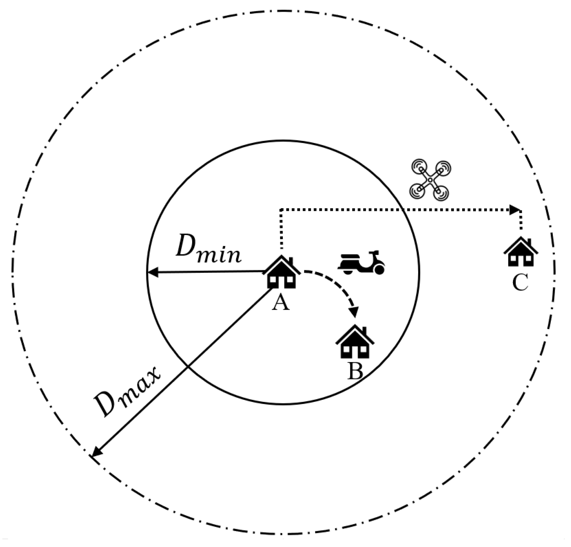
3.1. Problem Definition

We consider a multi-location assortment planning problem under the cooperative delivery by drone and human courier. We use $S_i$ to denote the assortment list for online store i, and the geographical regions are divided into M parts, $i\in M,M=\{1,\dots ,m\}$. The ratio of customers visiting an online retailer i is denoted by ${\theta }_i$ and satisfies ${\sum }_{i\in M}{\theta }_i=1$. The products are denoted by $N=\{1,\dots ,n\}$, and the online assortment consists of part of N. Customers can order a product in any online shop if it can be delivered to the spot where the customer is. Customers from spot $k,k\in M$ want to purchase a product in an online shop $i,i\in M$ according to the MNL model. In online store i with assortment $S_i$, the preference of product $j\in S_i$ delivered to spot k is $u_{ik}^j$, $u_i^0$ for the no-purchase option. Customers from spot k who visit online store i only consider the products in $S_i$ that can be delivered to k, and buy product j with probability $u_{ik}^j/(u_i^0+{\sum }_{l\in S_i^k}{u}_{ik}^l)$ or leave without buy anything with probability $u_i^0/(u_i^0+{\sum }_{l\in S_i^k}{u}_{ik}^l)$, $s_i^k$ meaning the products in $S_i$ can be delivered to spot k as well. Once the customer buys the product, the order will be served by drone or human courier. A drone can deliver goods within $D_{max}$ and more than $D_{min}$; a human courier can deliver goods within $D_{min}$. Figure 1 shows the distribution mode. We denote the marginal revenue of product j in online shop i is $r_i^j$, $j\in N$, the expected revenue of demand from spot k to online store i is ${\sum }_{l\in S_i^k}{r}_i^l{u}_{ik}^l/(u_i^0+{\sum }_{l\in S_i^k}{u}_{ik}^l)$. We define variable ${\gamma }_{ik}^j$ to be 1 if product j can be delivered from spot i to k, $i\in M,k\in M,j\in N$, and 0 otherwise. Variable $x_i^j=1$ when product i is provided in $S_i$, and 0 otherwise. We define variable $y_{ik}^j$ as equal to 1 if product j can be delivered from spot i to k using a drone, and 0 otherwise. Similarly, variable $z_{ik}^j$ is equal to 1 if product j can be delivered from spot i to k by human courier, and 0 otherwise. By introducing these binary variables, our MADH problem can be formulated as (1)–(8). We summarize all the other symbols in

Table 2. Nomenclature.

Notation	Description
$x_i^j$	1 if products j is provided in the online store i and 0 otherwise
$y_{ik}^j$	1 if product j can be delivered from spot i to k by drone and 0 otherwise
$z_{ik}^j$	1 if product j can be delivered from spot i to k by human courier and 0 otherwise
${\theta }_i$	Probability of demand for spot i
${\gamma }_{ik}^j$	Decision variable ${\gamma }_{ik}^j$ be 1 if product j can be delivered from spot i to k and 0 otherwise
$u_{ik}^j$	Preference associated with product j in assortment $S_i$ for demand from spot k
$u_i^0$	No-purchase preference of spot i
$r_i^j$	Marginal revenue of product j in spot i
W	Drone load capacity
$c_i$	The cardinality capacity of products in spot i
$w_j$	The weight of product j
$D_{max}$	Maximum delivery distance of the drone
$D_{min}$	Maximum delivery distance of the human courier

.

$$\begin{array}{cc}\hfill \pi =& max\sum _{i\in M}{\theta }_i\frac{{\sum }_{k\in M}{\sum }_{j\in N}{r}_i^j{u}_{ik}^j{\gamma }_{ik}^j}{u_i^0+{\sum }_{k\in M}{\sum }_{j\in N}{u}_{ik}^j{\gamma }_{ik}^j}\hfill \\ \hfill s.t.& \hfill \end{array}$$

(1)

$$\begin{array}{cc}\hfill & {\gamma }_{ik}^j=y_{ik}^j+z_{ik}^j,i\in M,j\in N,k\in M\hfill \end{array}$$

(2)

$$\left\{\begin{array}{c}if{d}_{ik}\in (D_{min},D_{max}),y_{ik}^j=1,i\in M,j\in N,k\in M\hfill \\ if{d}_{ik}\le D_{min},y_{ik}^j=0,i\in M,j\in N,k\in M\hfill \\ else{y}_{ik}^j=0,i\in M,j\in N,k\in M\hfill \end{array}\right.$$

(3)

$$\begin{array}{cc}\hfill & z_{ik}^j{d}_{ik}\le D_{min},i\in M,j\in N,k\in M\hfill \end{array}$$

(4)

$$\begin{array}{cc}\hfill & w_j{y}_{ik}^j\le W,i\in M,j\in N,k\in M\hfill \end{array}$$

(5)

$$\begin{array}{cc}\hfill & \sum _{j\in N}{x}_i^j\le c_i,i\in M\hfill \end{array}$$

(6)

$$\begin{array}{cc}\hfill & x_i^j\ge {\gamma }_{ik}^j,i\in M,j\in N,k\in M\hfill \end{array}$$

(7)

$$\begin{array}{cc}\hfill & x_i^j,y_{ik}^j,z_{ik}^j,{\gamma }_{ik}^j\in \{0,1\},i\in M,j\in N,k\in M\hfill \end{array}$$

(8)

The problem is to determine the optimal assortment of products for $\{S_1,\dots ,S_m\}$ to maximize the total revenue of the online retailer.

Equation (2) constrains the delivery of product j from i to k. If it can be delivered by drone or human courier, then ${\gamma }_{ik}^j=1$. Equation (3) means the delivery distance of the drone is within $D_{max}$ and more than $D_{min}$. Equation (4) means the delivery distance of a human courier is within $D_{min}$. Equation (5) means the product delivered by a drone cannot exceed the load capacity of the drone. Equation (6) is the cardinality constraint of the product in $S_i$. Equation (7) ensures that only the assortment $S_i$ include the product j, then it can be delivered to other location.

Based on the above equations, for Equation (3), we must add another two auxiliary binary variables $s_{ik}^j$, $t_{ik}^j$ which satisfy the following five equations where M is a big value. Then, Equation (3) can be expressed as Equations (9)–(14).

$$\begin{array}{cc}\hfill (Drone& deliveryconstraints)\hfill \end{array}$$

$$\begin{array}{cc}\hfill & s_{ik}^j+t_{ik}^j=2y_{ik}^j,i\in M,j\in N,k\in M\hfill \end{array}$$

(9)

$$\begin{array}{cc}\hfill & D_{min}<d_{ik}+M(1-s_{ik}^j),i\in M,j\in N,k\in M\hfill \end{array}$$

(10)

$$\begin{array}{cc}\hfill & D_{min}\ge d_{ik}-M{s}_{ik}^j,i\in M,j\in N,k\in M\hfill \end{array}$$

(11)

$$\begin{array}{cc}\hfill & D_{max}>d_{ik}-M(1-t_{ik}^j),i\in M,j\in N,k\in M\hfill \end{array}$$

(12)

$$\begin{array}{cc}\hfill & D_{max}\le d_{ik}+M{t}_{ik}^j,i\in M,j\in N,k\in M\hfill \end{array}$$

(13)

$$\begin{array}{cc}\hfill & s_{ik}^j,t_{ik}^j\in \{0,1\},i\in M,j\in N,k\in M\hfill \end{array}$$

(14)

3.2. Complexity

Lemma 1 

(Complexity). The multi-location assortment optimization problem under the cooperative delivery by drone and human courier is NP-hard.

Proof. 

For only one online store $M^{{}^{\prime }}=\left\{1\right\}$ and the products from it being delivered to spot $k,k\in M,M=\{1,\dots ,m\}$, the problem (1) can be reduced to the assortment problem with a single location under the MMNL model. The problem is proven to be NP-hard to approximate [41]. □

4. Mixed-Integer Linear Programming Formulation

In this section, we first convert the MADH problem into the MILP formulation in Section 4.1 and transfer it to the conic quadratic mixed 0–1 program in Section 4.2, then we strengthen it using McCormick inequalities in Section 4.3.

4.1. MILP Formulation

The above generic model (1)–(14) can be transformed into a linear program. To do that, we need to linearize the terms in the objective function of the above mathematical program. First, let $p_i=1/(u_i^0+{\sum }_{k\in M}{\sum }_{j\in N}{u}_{ik}^j{\gamma }_{ik}^j)$; by doing that, the objective function (1) becomes

$$\begin{array}{c}\hfill max\sum _{i\in M}\sum _{k\in M}\sum _{j\in N}{\theta }_i{r}_i^j{u}_{ik}^j{\gamma }_{ik}^j{p}_i\end{array}$$

(15)

Then, we linearize the bilinear term ${\gamma }_{ik}^j{p}_i$. We define new continuous variable $q_{ik}^j={\gamma }_{ik}^j{p}_i$ and add the following inequalities (16)–(18) to the formulation.

$$\begin{array}{cc}\hfill p_i-q_{ik}^j& \le M-M{\gamma }_{ik}^j,i\in M,j\in N,k\in M\hfill \end{array}$$

(16)

$$\begin{array}{cc}\hfill 0\le q_{ik}^j& \le p_i,i\in M,j\in N,k\in M\hfill \end{array}$$

(17)

$$\begin{array}{cc}\hfill q_{ik}^j& \le M{\gamma }_{ik}^j,i\in M,j\in N,k\in M\hfill \end{array}$$

(18)

where M is a sufficiently large number. We can replace M with an upper bound on $1/u_i^0$. The final MILP formulation can be expressed as (19)–(36)

$$\begin{array}{cc}\hfill \pi *=& max\sum _{i\in M}\sum _{k\in M}\sum _{j\in N}{\theta }_i{r}_i^j{u}_{ik}^j{q}_{ik}^j\hfill \\ \hfill s.t.& \hfill \end{array}$$

(19)

$$\begin{array}{cc}\hfill & {\gamma }_{ik}^j=y_{ik}^j+z_{ik}^j,i\in M,j\in N,k\in M\hfill \\ \hfill (Dronedelivery& constraints)\hfill \end{array}$$

(20)

$$\begin{array}{cc}\hfill & s_{ik}^j+t_{ik}^j=2y_{ik}^j,i\in M,j\in N,k\in M\hfill \end{array}$$

(21)

$$\begin{array}{cc}\hfill & D_{min}<d_{ik}+M(1-s_{ik}^j),i\in M,j\in N,k\in M\hfill \end{array}$$

(22)

$$\begin{array}{cc}\hfill & D_{min}\ge d_{ik}-M{s}_{ik}^j,i\in M,j\in N,k\in M\hfill \end{array}$$

(23)

$$\begin{array}{cc}\hfill & D_{max}>d_{ik}-M(1-t_{ik}^j),i\in M,j\in N,k\in M\hfill \end{array}$$

(24)

$$\begin{array}{cc}\hfill & D_{max}\le d_{ik}+M{t}_{ik}^j,i\in M,j\in N,k\in M\hfill \end{array}$$

(25)

$$\begin{array}{cc}\hfill & z_{ik}^j{d}_{ik}\le D_{min},i\in M,j\in N,k\in M\hfill \end{array}$$

(26)

$$\begin{array}{cc}\hfill & w_j{y}_{ik}^j\le W,i\in M,j\in N,k\in M\hfill \end{array}$$

(27)

$$\begin{array}{cc}\hfill & \sum _{j\in N}{x}_i^j\le c_i,i\in M\hfill \end{array}$$

(28)

$$\begin{array}{cc}\hfill & x_i^j\ge {\gamma }_{ik}^j,i\in M,j\in N,k\in M\hfill \end{array}$$

(29)

$$\begin{array}{cc}\hfill & u_i^0{p}_i+\sum _{k\in M}\sum _{j\in N}{u}_{ik}^j{q}_{ik}^j=1,i\in M\hfill \end{array}$$

(30)

$$\begin{array}{cc}\hfill \left(MILPfor{q}_{ik}^j\right)& u_i^0(p_i-q_{ik}^j)\le 1-{\gamma }_{ik}^j,i\in M,j\in N,k\in M\hfill \end{array}$$

(31)

$$\begin{array}{cc}\hfill & 0\le q_{ik}^j\le p_i,i\in M,j\in N,k\in M\hfill \end{array}$$

(32)

$$\begin{array}{cc}\hfill & u_i^0{q}_{ik}^j\le {\gamma }_{ik}^j,i\in M,j\in N,k\in M\hfill \end{array}$$

(33)

$$\begin{array}{cc}\hfill & p_i,q_{ik}^j\ge 0,i\in M,j\in N,k\in M\hfill \end{array}$$

(34)

$$\begin{array}{cc}\hfill & s_{ik}^j,t_{ik}^j\in \{0,1\},i\in M,j\in N,k\in M\hfill \end{array}$$

(35)

$$\begin{array}{cc}\hfill & x_i^j,y_{ik}^j,z_{ik}^j,{\gamma }_{ik}^j\in \{0,1\},i\in M,k\in M,j\in N\hfill \end{array}$$

(36)

4.2. Conic Formulation

Conic optimization has recently proven valid for the assortment planning problem in [33,34]. This work also used this method to achieve the purpose of accelerating calculation. We reformulate the objective function (1) as a conic formulation (37). Let ${\overline{r}}_i={max}_{j\in N}{r}_i^j$); instead of maximizing the revenue, we minimize the gap between the maximum possible gain by selling only the product with the highest revenue to an arriving customer $\left({\sum }_{i\in M}{\theta }_i{\overline{r}}_i\right)$.

$$\begin{array}{cc}\hfill max& \sum _{i\in M}{\theta }_i{\overline{r}}_i-\sum _{i\in M}\left[\frac{{\theta }_i{u}_i^0{\overline{r}}_i}{u_i^0+{\sum }_{k\in M}{\sum }_{j\in N}{u}_{ik}^j{\gamma }_{ik}^j}\right]-\sum _{i\in M}\sum _{k\in M}\sum _{j\in N}\left[\frac{{\theta }_i{u}_{ik}^j({\overline{r}}_i-r_i^j){\gamma }_{ik}^j}{u_i^0+{\sum }_{k\in M}{\sum }_{j\in N}{u}_{ik}^j{\gamma }_{ik}^j}\right]\hfill \end{array}$$

(37)

We assume $p_i=1/(u_i^0+{\sum }_{k\in M}{\sum }_{j\in N}{u}_{ik}^j{\gamma }_{ik}^j)$, $q_{ik}^j={\gamma }_{ik}^j{p}_i$ to linearize the problem as well, the maximization problem becomes the conic quadratic mixed 0–1 program as per (38)–(55):

$$\begin{array}{cc}\hfill \Omega =& min\sum _{i\in M}{\theta }_i{u}_i^0{\overline{r}}_i{p}_i+\sum _{i\in M}\sum _{k\in M}\sum _{j\in N}{\theta }_i{u}_{ik}^j({\overline{r}}_i-r_i^j)q_{ik}^j\hfill \\ \hfill s.t.& \hfill \end{array}$$

(38)

$$\begin{array}{cc}\hfill & {\gamma }_{ik}^j=y_{ik}^j+z_{ik}^j,i\in M,j\in N,k\in M\hfill \\ \hfill (Drone& deliveryconstraints)\hfill \end{array}$$

(39)

$$\begin{array}{cc}\hfill & s_{ik}^j+t_{ik}^j=2y_{ik}^j,i\in M,j\in N,k\in M\hfill \end{array}$$

(40)

$$\begin{array}{cc}\hfill & D_{min}<d_{ik}+M(1-s_{ik}^j),i\in M,j\in N,k\in M\hfill \end{array}$$

(41)

$$\begin{array}{cc}\hfill & D_{min}\ge d_{ik}-M{s}_{ik}^j,i\in M,j\in N,k\in M\hfill \end{array}$$

(42)

$$\begin{array}{cc}\hfill & D_{max}>d_{ik}-M(1-t_{ik}^j),i\in M,j\in N,k\in M\hfill \end{array}$$

(43)

$$\begin{array}{cc}\hfill & D_{max}\le d_{ik}+M{t}_{ik}^j,i\in M,j\in N,k\in M\hfill \end{array}$$

(44)

$$\begin{array}{cc}\hfill & z_{ik}^j{d}_{ik}\le D_{min},i\in M,j\in N,k\in M\hfill \end{array}$$

(45)

$$\begin{array}{cc}\hfill & w_j{y}_{ik}^j\le W,i\in M,j\in N,k\in M\hfill \end{array}$$

(46)

$$\begin{array}{cc}\hfill & \sum _{j\in N}{x}_i^j\le c_i,i\in M\hfill \end{array}$$

(47)

$$\begin{array}{cc}\hfill & x_i^j\ge {\gamma }_{ik}^j,i\in M,j\in N,k\in M\hfill \end{array}$$

(48)

$$\begin{array}{cc}\hfill & u_i^0{p}_i+\sum _{k\in M}\sum _{j\in N}{u}_{ik}^j{q}_{ik}^j\ge 1,i\in M\hfill \end{array}$$

(49)

$$\begin{array}{cc}\hfill \left(Conic\right)& o_i=u_i^0+\sum _{k\in M}\sum _{j\in N}{u}_{ik}^j{\gamma }_{ik}^j,i\in M\hfill \end{array}$$

(50)

$$\begin{array}{cc}\hfill & p_i{o}_i\ge 1,i\in M\hfill \end{array}$$

(51)

$$\begin{array}{cc}\hfill & q_{ik}^j{o}_i\ge {\gamma }_{ik}^{j^2},i\in M,j\in N,k\in M\hfill \end{array}$$

(52)

$$\begin{array}{cc}\hfill & p_i,q_{ik}^j\ge 0,i\in M,j\in N,k\in M\hfill \end{array}$$

(53)

$$\begin{array}{cc}\hfill & s_{ik}^j,t_{ik}^j\in \{0,1\},i\in M,j\in N,k\in M\hfill \end{array}$$

(54)

$$\begin{array}{cc}\hfill & x_i^j,y_{ik}^j,z_{ik}^j,{\gamma }_{ik}^j\in \{0,1\},i\in M,k\in M,j\in N\hfill \end{array}$$

(55)

4.3. McCormick Inequalities

We can further strengthen our formulation using McCormick inequalities for the bilinear term $q_{ik}^j$. If ${\gamma }_{ik}^j=0$. When calculating the lower bound of $p_i$, we first calculate the summation of ${\sum }_{k\in M}{u}_{ik}^j{\gamma }_{ik}^j,j\in N$ and sort the summary. The product with a higher summary will be added in the denominator of the fraction of $p_{i|{\gamma }_{ik}^j=0}^l$ when there still exists capacity. Therefore, there are two scenarios. One is when the preference summary of product j, ${\sum }_{\delta \in M^{-k}}{u}_{i\delta }^j$ in online store i is high enough to add to the assortment $S_i$, then it will be added into the denominator. In addition, the lower bound is as follows:

$$\begin{array}{cc}\hfill p_{i|{\gamma }_{ik}^j=0}^l:=& \frac{1}{u_i^0+{\sum }_{\delta \in M^{-k}}{u}_{i\delta }^j+{\sum }_{l=1}^{c_i-1}{\left({\sum }_{k=1}^m{u}_{ik}^{-j}\right)}_l}\le p_i,\hfill \end{array}$$

(56)

Otherwise, product j is not included in online store i, and the lower bound becomes

$$\begin{array}{cc}\hfill p_{i|{\gamma }_{ik}^j=0}^l:=& \frac{1}{u_i^0+{\sum }_{l=1}^{c_i}{\left({\sum }_{k=1}^m{u}_{ik}^{-j}\right)}_l}\le p_i\hfill \end{array}$$

(57)

The upper bound (58) assumes no product in the assortment $S_i$.

$$\begin{array}{cc}\hfill p_{i|{\gamma }_{ik}^j=0}^u:=& \frac{1}{u_i^0}\ge p_i\hfill \end{array}$$

(58)

If ${\gamma }_{ik}^j=1$, the lower bound of $p_i$ is as per (59), which means the product j is included in $S_i$ and can be delivered to any location $k,k\in M$. The upper bound (60) means the product is included in the $S_i$ and only can be delivered to location k. ${\sum }_{l=1}^{c_i-1}{\left({\sum }_{k=1}^m{u}_{ik}^{-j}\right)}_l$ is the summary of the former $c_i-1$ largest summation of $u_{ik}^{\xi },\xi \in N\backslash j$. $M^{-k}$ is the spot set without k.

$$\begin{array}{cc}\hfill p_{i|{\gamma }_{ik}^j=1}^l:=& \frac{1}{u_i^0+{\sum }_{k=1}^m{u}_{ik}^j+{\sum }_{l=1}^{c_i-1}{\left({\sum }_{k=1}^m{u}_{ik}^{-j}\right)}_l}\le p_i\hfill \end{array}$$

(59)

$$\begin{array}{cc}\hfill p_{i|{\gamma }_{ik}^j=1}^u:=& \frac{1}{u_i^0+u_{ik}^j}\ge p_i\hfill \end{array}$$

(60)

From the introduced bounds (56)–(60), we can obtain valid McCormick inequalities for each bilinear term $q_{ik}^j$.

$$\begin{array}{cc}\hfill q_{ik}^j& \le p_{i|{\gamma }_{ik}^j=1}^u·{\gamma }_{ik}^j,i\in M,j\in N,k\in M\hfill \end{array}$$

(61)

$$\begin{array}{cc}\hfill q_{ik}^j& \ge p_{i|{\gamma }_{ik}^j=1}^l·{\gamma }_{ik}^j,i\in M,j\in N,k\in M\hfill \end{array}$$

(62)

$$\begin{array}{cc}\hfill q_{ik}^j& \le p_i-p_{i|{\gamma }_{ik}^j=0}^l(1-{\gamma }_{ik}^j),i\in M,j\in N,k\in M\hfill \end{array}$$

(63)

$$\begin{array}{cc}\hfill q_{ik}^j& \ge p_i-p_{i|{\gamma }_{ik}^j=0}^u(1-{\gamma }_{ik}^j),i\in M,j\in N,k\in M\hfill \end{array}$$

(64)

5. Numerical Study

In our numerical study, we first test the performance of the conic optimization approach with McCormick inequalities. Then, we conduct two experiments to obtain some practical advice for drone delivery service. We fix the MADH problem using the Gurobi 9.5.2 solver on a computer with Intel Core i7-8700K 3.70 GHz processor and 64 GB RAM operating, and Windows 10 with the default settings of Gurobi.

5.1. Effectiveness of MILP and Conic + MC

In this subsection, we test the effectiveness of MILP and Conic + MC. First, we set $d_{ik}=d_{ki},i\in M,k\in M$ from a uniform U[1, 20] distribution and $d_{ii}=0,i\in M$. The $D_{max}$ and $D_{min}$ are 6 and 3, the weight of product $w_j,j\in N$ and marginal revenue $r_i^j=r_j,i\in M,j\in N$ from a uniform U[1, 5] distribution, respectively. The load capacity of a drone W is 3. To produce the arrival rate ${\theta }_i$ of online store $i,i\in M$, we generate ${\alpha }_i$ from the uniform distribution over [0, 1] for all $i=1,\dots ,m$. Then, we set ${\theta }_i={\alpha }_i/{\sum }_{i=1}^m\left({\alpha }_i\right)$.

In

Table 3. Effectiveness of MILP and Conic + MC.

M	N	${\mathit{c}}_{\mathit{i}}$	${\mathit{u}}_{\mathit{i}}^0$	${\mathit{u}}_{\mathit{ik}}^{\mathit{j}}$	MILP			Conic + MC
					Value	CPU/s	Gap	Value	CPU/s
10	200	[10, 12]	20	[0, 1]	2.416	600	5.57 × 10${}^{-6}$	2.416	13.086
15					2.758	600	3.36 × 10${}^{-5}$	2.758	57.993
20					2.968	600	6.78 × 10${}^{-6}$	2.968	161.322
25					3.199	600	2.57 × 10${}^{-5}$	3.199	310.179
30					3.352	600	5.03 × 10${}^{-6}$	3.352	372.597
20	100	[10, 12]	20	[0, 1]	2.869	600	5.08 × 10${}^{-7}$	2.869	42.040
	120				2.837	600	1.92 × 10${}^{-5}$	2.837	65.766
	140				2.939	600	7.33 × 10${}^{-8}$	2.939	80.716
	160				2.929	600	3.77 × 10${}^{-5}$	2.929	88.233
	180				2.956	600	3.21 × 10${}^{-5}$	2.956	113.929
	200				2.969	600	1.72 × 10${}^{-6}$	2.969	127.364
20	200	[4, 6]	20	[0, 1]	2.272	600	6.10 × 10${}^{-8}$	2.272	29.100
		[6, 8]			2.507	600	6.32 × 10${}^{-6}$	2.507	52.958
		[8, 10]			2.800	600	9.89 × 10${}^{-6}$	2.800	64.435
		[10, 12]			3.014	600	5.82 × 10${}^{-7}$	3.014	140.901
		[12, 14]			3.137	600	2.91 × 10${}^{-5}$	3.137	259.235
		[14, 16]			3.254	600	4.20 × 10${}^{-6}$	3.254	343.928
20	200	[10, 12]	10	[0, 1]	3.611	600	1.18 × 10${}^{-5}$	3.611	220.315
			20		2.804	600	6.77 × 10${}^{-6}$	2.804	108.650
			30		2.499	600	7.72 × 10${}^{-7}$	2.499	83.416
			40		2.274	600	2.02 × 10${}^{-6}$	2.274	74.115
			50		1.962	600	9.75 × 10${}^{-8}$	1.962	65.058
20	200	[10, 12]	20	[0, 1]	2.820	600	5.84 × 10${}^{-7}$	2.820	116.823
				[1, 2]	3.885	600	2.69 × 10${}^{-6}$	3.885	209.405
				[2, 3]	4.294	600	5.33 × 10${}^{-6}$	4.294	170.582
				[3, 4]	4.408	600	1.31 × 10${}^{-5}$	4.408	95.440
				[4, 5]	4.492	600	8.11 × 10${}^{-8}$	4.492	178.419

, we vary five different parameters, which are the number of stores M, varying from one of these possible values: $\{10,15,20,25,30\}$; and the number of products N, varying from one of these possible values: $\{100,120,140,160,180,200\}$. We set the cardinality constraints $c_i,i\in M$ of the online stores from the uniform distribution whose ranges are from $\left\{\right[4,6],[6,8],[8,10],[10,12],[12,14],[14,16\left]\right\}$; customers’ no-purchase preference on product $u_i^0$ vary from these values: $\{10,20,30,40,50\}$; and purchase preference $u_{ik}^j$ vary from the uniform distribution whose ranges are from $\left\{\right[0,1],[1,2],[2,3],[3,4],[4,5\left]\right\}$. Therefore, we have a total of 27 scenarios. We use MILP (19)–(36) and Conic + MC (38)–(64) to obtain the optimal valve and running 20 times, respectively. The gap equal to $(Valu{e}^{Conic+MC}-Valu{e}^{MILP})/Valu{e}^{Conic+MC}$. We set the time limit as 600s and show the effectiveness of MILP and Conic + MC in Table 3. From Table 3, we could safely conclude that Conic + MC performs better than MILP in these parameter settings. MILP can hardly finish computing in 600 s, even though the problem is easy to solve in Table 3 and Conic + MC solved the problem within 300 s. We can find that the optimal values between these two methods are roughly the same, but the Conic + MC that we propose for this MADH problem can obtain the optimal value much faster. The effectiveness of Conic + MC also shows that when the M, N, $c_i$ is bigger, the calculating time of Conic + MC is longer, and the calculation time is more sensitive to $c_i$ and M than N. When we change the $u_i^0$ and $u_{ik}^j$, the calculating time of Conic + MC is shorter when the $u_i^0$ becomes larger, but the calculating time increases first and then decreases with the increase of $u_{ik}^j$.

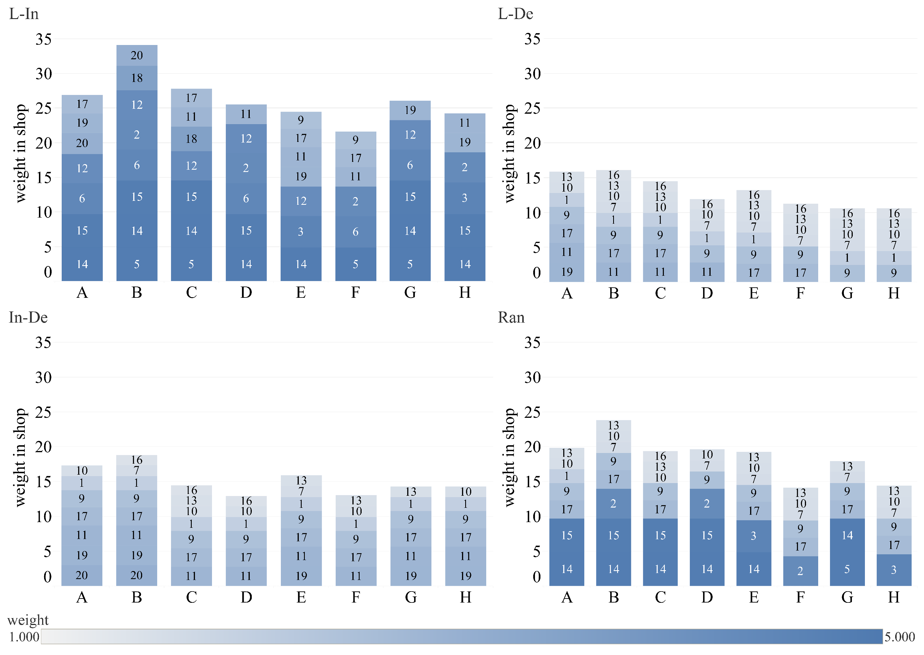
5.2. The Influence of Marginal Revenue Varying by Weight

In this subsection, we explore the influence of marginal revenue that varies according to the weight of the product. We assume there are eight spots (online stores) ranging from A to H, and 20 products. The capacity of each spot varies from $[6,8]$ in uniform distribution, $u_i^0=20$, $u_{ik}^j$ is of $[0,1]$ uniform distribution, $d_{ik}=d_{ki},i\in M,k\in M$ is of $[1,20]$ uniform distribution and $d_{ii}=0,i\in M$.

Table A1. Distance table.

	A	B	C	D	E	F	G	H	Capacity List
A	0.000	18.063	10.890	14.064	18.900	19.174	5.693	14.105	7
B	18.063	0.000	15.143	1.864	3.705	11.626	1.066	8.683	8
C	10.890	15.143	0.000	19.600	16.926	5.179	4.944	6.794	7
D	14.064	1.864	19.600	0.000	9.494	16.088	9.502	17.944	6
E	18.900	3.705	16.926	9.494	0.000	7.001	9.586	5.640	7
F	19.174	11.626	5.179	16.088	7.001	0.000	18.664	5.622	6
G	5.693	1.066	4.944	9.502	9.586	18.664	0.000	1.447	6
H	14.105	8.683	6.794	17.944	5.640	5.622	1.447	0.000	6

lists the details of these distances and the capacity of each spot. The $D_{max},D_{min}$, and W are 6, 3, and 3, respectively. We set $w_j$ to be of $[1,5]$ uniform distribution. We consider four scenarios where the $r_j$($r_i^j=r_j,i\in M,j\in N$) and $w_j,j\in N$ conform to the relation of linear–increasing, linear–decreasing, increasing–decreasing, and random. When the weight of product $w_j$ increases, we set $r_j=w_j$ as the linear–increasing scenario, set $r_j=-w_j+5$ as the linear–decreasing scenario, set $r_j=sin(\pi \ast w_j/5)\ast 5$ as the increasing–decreasing scenario, and $r_j$ is of $[1,5]$ uniform distribution in the random scenario.

Table A2. Revenue table.

Product	Weight	L–In	L–De	In–De	Ran	Product	Weight	L–In	L–De	In–De	Ran
1	1.987	1.987	3.013	4.743	2.069	11	2.828	2.828	2.172	4.894	1.064
2	4.317	4.317	0.683	2.079	3.592	12	4.241	4.241	0.759	2.296	1.262
3	4.586	4.586	0.414	1.284	4.964	13	1.528	1.528	3.472	4.097	3.888
4	3.112	3.112	1.888	4.635	4.163	14	4.849	4.849	0.151	0.474	4.152
5	4.856	4.856	0.144	0.453	3.586	15	4.831	4.831	0.169	0.531	3.680
6	4.471	4.471	0.529	1.633	2.572	16	1.462	1.462	3.538	3.974	2.651
7	1.600	1.600	3.400	4.222	4.422	17	2.646	2.646	2.354	4.979	4.486
8	3.105	3.105	1.895	4.643	1.248	18	3.523	3.523	1.477	4.002	3.295
9	2.462	2.462	2.538	4.999	4.629	19	2.841	2.841	2.159	4.886	2.113
10	1.564	1.564	3.436	4.161	3.490	20	3.003	3.003	1.997	4.753	1.639

lists the results of marginal revenues in different scenarios. For the convenience of expression, we denote them as L–In, L–De, In–De, and Ran. Figure 2 shows the results of our tests. It shows the weight distribution of products from A to H in four scenarios. The number in the middle of the rectangle represents the number of the product. Table A2 lists the product number and its weight. When the blue of the rectangle is darker, the product is heavier, as shown at the bottom of the Figure. The abscissa of each scenario represents the online store, and the vertical axis represents the product weight of each shop.

From Figure 2, we can find in the L–In scenario, the heavier product is more evenly distributed over the spots. On the contrary, the lighter product is more evenly distributed in the L–De scenario, and the product of moderate weight is more evenly distributed in the In–De scenario. In the Ran scenario, the product has the most evenly distributed weight. Therefore, we can put forward some management suggestions for weight–revenue-sensitive products. Retailers need to plan the distribution of products according to their weight more properly. For products whose marginal revenue and weight are positively correlated, such as some jewelry and small electronics that cost little in terms of storage, products with a high weight should be placed evenly in different locations. For products whose revenue and weight are negatively correlated, such as some huge home appliances that cost a lot in terms of storage, the lighter product should be evenly distributed. For some daily necessities that may show a characteristic of the In–De scenario because of its corruption, moderate-weight products are preferred in different locations. For the Ran case, products with different weights should be placed more evenly. Moreover, we can find that the maximum-weight product is not always distributed in all L–In stores, and the minimum-weight product is not always distributed in all L–De stores, which indicates that when the delivery weight is limited, the most profitable products do not have to be distributed in all stores. Therefore, considering delivery constraints, the reasonable arrangement of product assortment can improve retail revenue, especially in some chain stores.

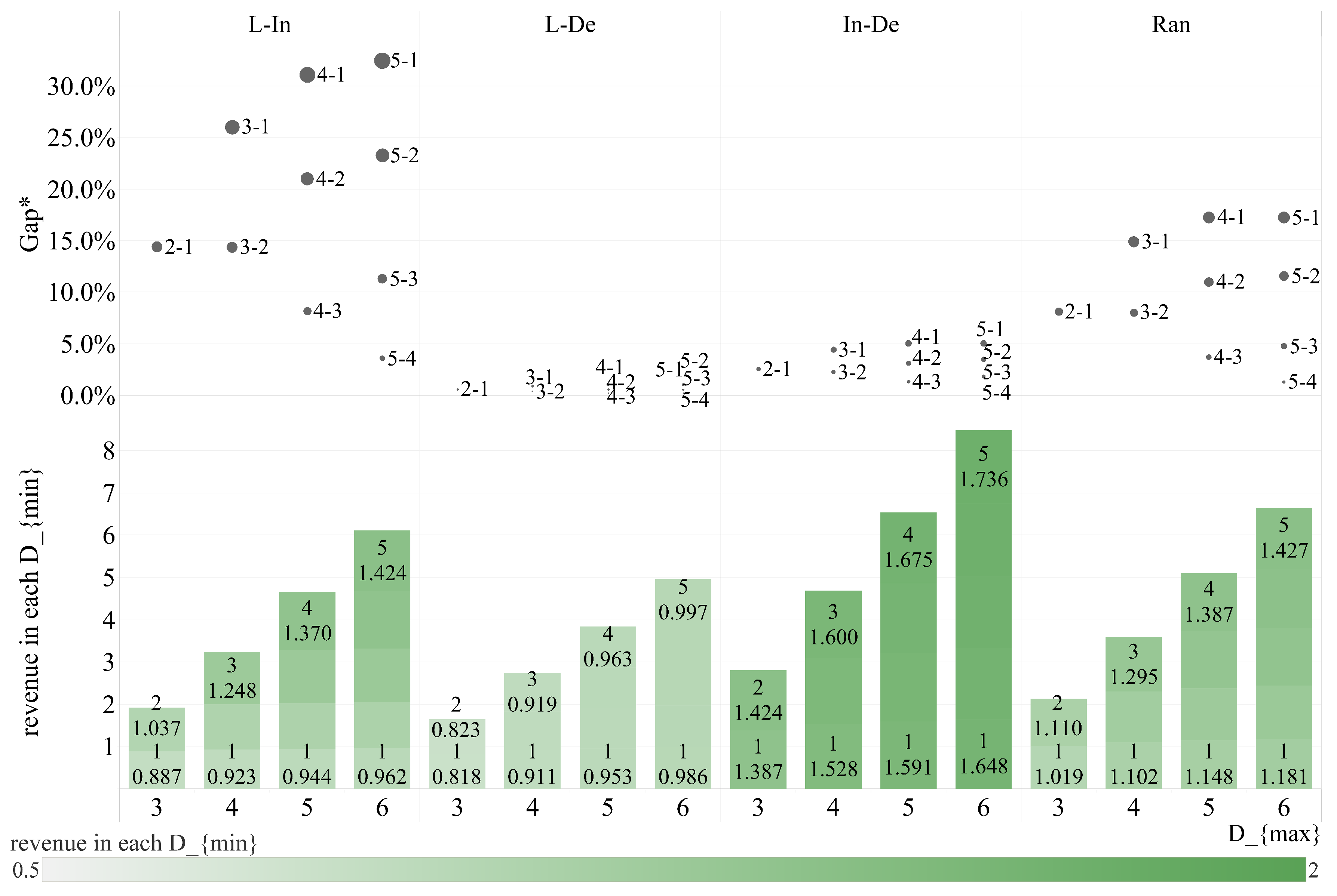
5.3. The Influence of Delivery Distance on Revenue

In this subsection, we consider the impact of delivery distance on the whole revenue, where the marginal revenue of a product varies from the four scenarios in Section 5.2. We use the same parameter settings as Section 5.2, and vary the $D_{max}$ and $D_{min}$ from $\{3,4,5,6\}$ and $\{1,2,3,4,5\}$. The results are shown in

Table 4. The revenue under different delivery distances and marginal revenues.

${\mathit{D}}_{\mathit{max}}$	3		4			5				6
${\mathit{D}}_{\mathit{min}}$	1	2	1	2	3	1	2	3	4	1	2	3	4	5
L–In	0.887	1.037	0.923	1.068	1.248	0.944	1.083	1.258	1.370	0.962	1.092	1.263	1.373	1.424
L–De	0.818	0.823	0.911	0.916	0.919	0.953	0.958	0.961	0.963	0.986	0.991	0.994	0.997	0.997
In–De	1.387	1.424	1.528	1.564	1.600	1.591	1.623	1.653	1.675	1.648	1.676	1.704	1.725	1.736
Ran	1.019	1.110	1.102	1.190	1.295	1.148	1.234	1.335	1.387	1.181	1.262	1.359	1.408	1.427

. There are also four weight-marginal revenue relations, namely L–In, L–De, In–De, and Ran, and Figure 3 is divided into four parts according to them. In each part, the abscissa represents $D_{max}$, the vertical above represents the $Ga{p}^{*}$, and below is the revenue in each $D_{min}$ for the same $D_{max}$. If we assume $D_{max}=D_{\alpha },D_{min}=D_{\beta }$, the revenue can be expressed as $R_{\alpha -\beta }$, then the $Ga{p}^{*}$ is equal to $(D_{\alpha -{\alpha }^{{}^{\prime }}\{{\alpha }^{{}^{\prime }}=\alpha -1\}}-D_{\alpha -\beta })/D_{\alpha -{\alpha }^{{}^{\prime }}\{{\alpha }^{{}^{\prime }}=\alpha -1\}}$ which is shown as a circle in the top half of each part and is numbered as ${\alpha }^{\prime }-\beta$. The size of the circle indicates the gap size. For the rectangle shown below, in the middle, the number above represents $D_{min}$, below is the retailers’ optimal revenue under this delivery setting, and we only show the maximization and minimization of it. Moreover, the width of the rectangle represents the revenue in each $D_{min}$ under this $D_{max}$. In addition, we use the depth of green to represent the revenue level under different $D_{max}$ and $D_{min}$ as shown at the bottom of the Figure.

From Figure 3, when $D_{max}$ is fixed, we can easily see that L–In and Ran offer obvious improvements to revenue if we improve the $D_{min}$, as the green grows darker and the $Ga{p}^{*}$ decreases quickly. Therefore, retailers can have a significant increase in revenue when they improve the $D_{min}$ in these two situations. In addition, the rate of gap reduction is not slowing down, which means the increase of $D_{min}$ is effective in obtaining a higher revenue for retailers. However, when In–De improves slightly, L–De is even less. Moreover, we can find when the $D_{max}$ grows bigger, the $Ga{p}^{*}$ increases fast in 3-1, and then the trends flatten out in all scenarios. This reflects that when $D_{max}$ is fixed, no matter what $D_{min}$ is, the $Ga{p}^{*}$ between $D_{max}-D_{max-1}$ and $D_{max}-1$ is within $40\%$ in the L–In situation, $5\%$ in L–De, $10\%$ in In–De and $20\%$ in Ran under this parameter setting. As the rate of gap reduction is not slowing down, one can speculate the $Ga{p}^{*}$ when the $D_{max}$ is given. Moreover, we can also conclude that in the L–In and Ran scenarios, $R_{\alpha -\beta }$ is larger than $R_{\alpha -{\beta }^{{}^{\prime }}\{{\beta }^{{}^{\prime }}<\beta \}}$, $R_{{\alpha }^{{}^{\prime }}\{{\alpha }^{{}^{\prime }}<\alpha \}-\beta }$ and $R_{{\alpha }^{{}^{\prime }}\{{\alpha }^{{}^{\prime }}>\alpha \}-{\beta }^{{}^{\prime }}\{{\beta }^{{}^{\prime }}<\beta \}}$ as the green is darker in $R_{\alpha -\beta }$ obviously. The L–De and In–De are also consistent with this conclusion, but the difference is relatively small. This principle shows that retailers can earn more by improving the $D_{min}$ slightly and fixing the $D_{max}$ or decreasing $D_{max}$ slightly to reduce the delivery cost.

6. Conclusions

This paper studies the problem of multi-location assortment planning under cooperative delivery by drone and human courier. We use the MMNL model to capture customer purchase behavior. We present a conic quadratic mixed-integer formulation of this problem and strengthen it using McCormick inequalities. We verify that our Conic + MC is effective, and we try to explore the weight distribution under four product marginal revenue structures and give some advice on assortment planning and distribution management for retailers. In general, this work can provide some suggestions for the commercial use of drones and enrich the study of assortment optimization under the MMNL model.

For future work, one direction is to consider different stores equipped with different delivery distances. Another direction is to consider other cooperative distribution modes such as truck–drone. Furthermore, our results may also provide some guidance for distribution network setup and revenue management research.

References

1. Jin. Meituan Drones: In 2022, More Than 100,000 Orders Were Delivered between Shanghai and Shenzhen, with an Average of 12 Minutes per Order. 2023. Available online: https://finance.sina.com.cn/jjxw/2023-01-16/doc-imyakpnk9115299.shtml (accessed on 16 January 2023).
2. Kirschstein, T. Comparison of energy demands of drone-based and ground-based parcel delivery services. Transp. Res. Part Transp. Environ. 2020, 78, 102209. [Google Scholar] [CrossRef]
3. Kim, S.H. Choice model based analysis of consumer preference for drone delivery service. J. Air Transp. Manag. 2020, 84, 101785. [Google Scholar] [CrossRef]
4. Borghetti, F.; Caballini, C.; Carboni, A.; Grossato, G.; Maja, R.; Barabino, B. The use of drones for last-mile delivery: A numerical case study in milan, italy. Sustainability 2022, 14, 1766. [Google Scholar] [CrossRef]
5. Lyu, G.; Teo, C.-P. Last mile innovation: The case of the locker alliance network. Manuf. Serv. Oper. Manag. 2022, 24, 2425–2443. [Google Scholar] [CrossRef]
6. Clothier, R.A.; Greer, D.A.; Greer, D.G.; Mehta, A.M. Risk perception and the public acceptance of drones. Risk Anal. 2015, 35, 1167–1183. [Google Scholar] [CrossRef]
7. Waris, I.; Ali, R.; Nayyar, A.; Baz, M.; Liu, R.; Hameed, I. An empirical evaluation of customers’ adoption of drone food delivery services: An extended technology acceptance model. Sustainability 2022, 14, 2922. [Google Scholar] [CrossRef]
8. Aydin, B. Public acceptance of drones: Knowledge, attitudes, and practice. Technol. Soc. 2019, 59, 101180. [Google Scholar] [CrossRef]
9. Park, J.; Kim, S.; Suh, K. A comparative analysis of the environmental benefits of drone-based delivery services in urban and rural areas. Sustainability 2018, 10, 888. [Google Scholar] [CrossRef]
10. Baldisseri, A.; Siragusa, C.; Seghezzi, A.; Mangiaracina, R.; Tumino, A. Truck-based drone delivery system: An economic and environmental assessment. Transp. Res. Part Transp. Environ. 2022, 107, 103296. [Google Scholar] [CrossRef]
11. Chauhan, D.; Unnikrishnan, A.; Figliozzi, M. Maximum coverage capacitated facility location problem with range constrained drones. Transp. Res. Part Emerg. Technol. 2019, 99, 1–18. [Google Scholar] [CrossRef]
12. Cicek, C.T.; Gultekin, H.; Tavli, B. The location-allocation problem of drone base stations. Comput. Oper. Res. 2019, 111, 155–176. [Google Scholar] [CrossRef]
13. Aurambout, J.-P.; Gkoumas, K.; Ciuffo, B. Last mile delivery by drones: An estimation of viable market potential and access to citizens across european cities. Eur. Transp. Res. Rev. 2019, 11, 30. [Google Scholar] [CrossRef]
14. Salama, M.; Srinivas, S. Joint optimization of customer location clustering and drone-based routing for last-mile deliveries. Transp. Res. Part Emerg. Technol. 2020, 114, 620–642. [Google Scholar] [CrossRef]
15. Poikonen; S; Golden; B Multi-visit drone routing problem. Comput. Oper. Res. 2020, 113, 104802. [CrossRef]
16. Wang, Z.; Sheu, J.-B. Vehicle routing problem with drones. Transp. Res. Part Methodol. 2019, 122, 350–364. [Google Scholar] [CrossRef]
17. Sadiq, O.B.; Salawudeen, A. Fanet optimization: A destination path flow model. Int. J. Electr. Comput. Eng. (IJECE) 2020, 10, 4381–4389. [Google Scholar] [CrossRef]
18. Poikonen, S.; Golden, B. The mothership and drone routing problem. Informs J. Comput. 2020, 32, 249–262. [Google Scholar] [CrossRef]
19. Leon-Blanco, J.M.; Gonzalez-R, P.L.; Andrade-Pineda, J.L.; Canca, D.; Calle, M. A multi-agent approach to the truck multi-drone routing problem. Expert Syst. Appl. 2022, 195, 116604. [Google Scholar] [CrossRef]
20. Chung, S.H.; Sah, B.; Lee, J. Optimization for drone and drone-truck combined operations: A review of the state of the art and future directions. Comput. Oper. Res. 2020, 123, 105004. [Google Scholar] [CrossRef]
21. Talluri, K.; Van Ryzin, G. Revenue management under a general discrete choice model of consumer behavior. Manag. Sci. 2004, 5, 15–33. [Google Scholar] [CrossRef]
22. Rusmevichientong, P.; Shen, Z.-J.M.; Shmoys, D.B. Dynamic assortment optimization with a multinomial logit choice model and capacity constraint. Oper. Res. 2010, 58, 1666–1680. [Google Scholar] [CrossRef]
23. Davis, J.; Gallego, G.; Topaloglu, H. Assortment planning under the multinomial logit model with totally unimodular constraint structures. In Work in Progress; Department of IEOR, Columbia University: Palisades, NY, USA, 2013. [Google Scholar]
24. Feldman, J.; Paul, A. Relating the approximability of the fixed cost and space constrained assortment problems. Prod. Oper. Manag. 2019, 28, 1238–1255. [Google Scholar] [CrossRef]
25. Davis, J.M.; Gallego, G.; Topaloglu, H. Assortment optimization under variants of the nested logit model. Oper. Res. 2014, 62, 250–273. [Google Scholar] [CrossRef]
26. Gallego, G.; Topaloglu, H. Constrained assortment optimization for the nested logit model. Manag. Sci. 2014, 60, 2583–2601. [Google Scholar] [CrossRef]
27. Feldman, J.; Topaloglu, H. Capacitated assortment optimization under the multinomial logit model with nested consideration sets. Oper. Res. 2018, 66, 380–391. [Google Scholar] [CrossRef]
28. Rusmevichientong, P.; Shmoys, D.; Topaloglu, H. Assortment optimization with mixtures of logits. In Technical Report; School of IEOR, Cornell University: Ithaca, NY, USA, 2010. [Google Scholar]
29. Mittal, S.; Schulz, A.S. A general framework for designing approximation schemes for combinatorial optimization problems with many objectives combined into one. Oper. Res. 2013, 61, 386–397. [Google Scholar] [CrossRef]
30. Désir, A.; Goyal, V.; Zhang, J. Near-optimal algorithms for capacity constrained assortment optimization. SSRN 2014, 2543309. [Google Scholar] [CrossRef]
31. Bront, J.J.M.; Méndez-Díaz, I.; Vulcano, G. A column generation algorithm for choice-based network revenue management. Oper. Res. 2009, 57, 769–784. [Google Scholar] [CrossRef]
32. Méndez-Díaz, I.; Miranda-Bront, J.J.; Vulcano, G.; Zabala, P. A branch-and-cut algorithm for the latent-class logit assortment problem. Discret. Appl. Math. 2014, 164, 246–263. [Google Scholar] [CrossRef]
33. Bebitoğlu, B. Multi-Location Assortment Optimization under Capacity Constraints. Ph.D. Thesis, Bilkent Universitesi, Ankara, Turkey, 2016. [Google Scholar]
34. Sen, A.; Atamturk, A.; Kaminsky, P. A conic integer optimization approach to the constrained assortment problem under the mixed multinomial logit model. Oper. Res. 2018, 66, 994–1003. [Google Scholar] [CrossRef]
35. Chen, J.; Liang, Y.; Shen, H.; Shen, Z.-J.M.; Xue, M. Offline-channel planning in smart omnichannel retailing. Manuf. Serv. Oper. Manag. 2022, 24, 2444–2462. [Google Scholar] [CrossRef]
36. Akçay, Y.; Tan, B. On the benefits of assortment-based cooperation among independent producers. Prod. Oper. Manag. 2008, 17, 626–640. [Google Scholar] [CrossRef]
37. Besbes, O.; Sauré, D. Product assortment and price competition under multinomial logit demand. Prod. Oper. Manag. 2016, 25, 114–127. [Google Scholar] [CrossRef]
38. Rodríguez, B.; Aydın, G. Pricing and assortment decisions for a manufacturer selling through dual channels. Eur. J. Oper. Res. 2015, 242, 901–909. [Google Scholar] [CrossRef]
39. Gallego, G.; Li, A.; Truong, V.-A.; Wang, X. Approximation algorithms for product framing and pricing. Oper. Res. 2020, 68, 134–160. [Google Scholar] [CrossRef]
40. Lin, Y.H.; Wang, Y.; He, D.; Lee, L.H. Last-mile delivery: Optimal locker location under multinomial logit choice model. Transp. Res. Part Logist. Transp. Rev. 2020, 142, 102059. [Google Scholar] [CrossRef]
41. Désir, A.; Goyal, V.; Zhang, J. Capacitated assortment optimization: Hardness and approximation. Oper. Res. 2022, 70, 893–904. [Google Scholar] [CrossRef]
Figure 1. Delivery range of drone and human courier.
Applsci 13 05441 g001
Figure 2. Weight distribution of four scenarios.
Applsci 13 05441 g002
Figure 3. Impacts of delivery distance.
Applsci 13 05441 g003