Article

A 2.5D Finite Element Method Combined with Zigzag-Paraxial Boundary for Long Tunnel under Obliquely Incident Seismic Wave

1
The Key Laboratory of Urban Security and Disaster Engineering, Ministry of Education, Beijing University of Technology, Beijing 100124, China
2
The Beijing Key Laboratory of Urban Underground Space Engineering, School of Civil and Resource Engineering, University of Science and Technology Beijing, Beijing 100083, China
3
Department of Hydraulic Engineering, Tsinghua University, Beijing 100084, China
*
Author to whom correspondence should be addressed.
Appl. Sci. 2023, 13(9), 5743; https://doi.org/10.3390/app13095743
Submission received: 24 March 2023 / Revised: 1 May 2023 / Accepted: 5 May 2023 / Published: 6 May 2023
(This article belongs to the Special Issue Geotechnical Earthquake Engineering: Current Progress and Road Ahead)

Abstract

:
Seismic waves propagation with an oblique angle to the tunnel axis will cause asynchronous tunnel motions and have a significant effect on the axial response. A high-precision 2.5D finite element method is established in the frequency domain to simulate the 3D seismic response of the tunnel. This method avoids the disturbance caused by the truncation of the tunnel in the longitudinal direction. Meanwhile, a 2.5D zigzag-paraxial boundary is derived to further improve the calculation efficiency of the 2.5D finite element model. Moreover, by combining the 2.5D finite element method, 2.5D zigzag boundary condition and seismic motion input methods, an obliquely incident substructure method for plane seismic waves is built by converting the plane seismic wave into equivalent nodal forces. The proposed 2.5D finite element method is verified by comparing with a reference solution. Finally, the 2.5D finite element method is applied to study the seismic response of the long lined tunnel. Parameter analyses illustrate that the wave propagation effect to the tunnel axis has a non-negligible influence on the axil deformation of long tunnels.

1. Introduction

In seismic engineering problems, the study of tunnel dynamic characteristics has become increasingly important. The safety of tunnels under earthquakes has attracted extensive attention [1,2,3,4,5]. Some observation results show that when seismic wave propagates along the longitudinal direction, it will cause tension, compression and bending deformation of the tunnel [6]. As an underground structure with a large span in the longitudinal direction, tunnel deformation in the longitudinal direction is more remarkable than that in the transverse direction, which should be highly considered in seismic design.
The common seismic analysis methods of underground tunnels include analytical solutions [7,8], model experiments [9] and numerical methods [10,11,12,13,14]. Compared with the assumption limitation of the analytical method and the long period of experimental testing, numerical methods can efficiently and accurately analyze complex soil–structure dynamic interaction. For a 3D simplified soil–tunnel model, soil around the tunnel is denoted by using soil springs to consider the soil–tunnel interaction [15]. Based on the concurrent discretization of the entire computation domain with coarse and fine-scale finite element meshes, Yu et al. [10] used a multi-scale method to simulate dynamic responses of a long tunnel. Li and Song [11] established a 3D soil–tunnel structure interaction model to simulate the longitudinal response of the tunnel when subjected to an asynchronous earthquake. Based on the time-domain finite element method with the viscous-spring artificial boundary condition, Huang et al. [13] conducted a study of the seismic responses of the long lined tunnels under the obliquely incident earthquake. Fabozzi et al. [12] addressed the problem of underground tunnels when subjected to asynchronous seismic shaking along the axis by a comparison with the synchronous case that is usually considered in the tunnel design. Both sides of the tunnel model are truncated, resulting in some numerical errors in the seismic response of the tunnel. Therefore, the 3D finite element model needs to take a long distance in the longitudinal direction to ensure that the tunnel seismic response results are accurate.
In recent years, some researchers have become increasingly interested in 2.5D modeling methods for tunnel–soil system dynamic interaction analysis, because in long lined tunnels, 2.5D finite element models are more efficient and accurate than 3D models. Hwang and Lysmer [16] first used a special type of wave transmission element to simplify the 3D system into a finite element plane, where each node of the plane element has three degrees of freedom, while retaining the propagation effects of waves. Yang and Hung [17] introduced the 2.5D method, which applies Fourier transform of the longitudinal coordinate to reduce the problem’s dimensionality and named it the 2.5D finite element/infinite element method. According to the different positions of the excitation source, the dynamic interaction analysis of the tunnel–soil system is mainly divided into two categories. One is the internal source problem, such as the vibration analysis of tunnel–soil system under moving train load [17,18,19,20,21,22,23,24,25]. Sheng et al. [19] coupled the finite element boundary element (FE–BE) method to analyze the vibration problem of the soil–tunnel system caused by moving trains load in the ground or tunnels. François et al. [20] studied the dynamic interaction between tunnels and layered soil under train load by using the general 2.5D FE-BE method. Jin et al. [22] used measurement data of dynamic response of tunnel to verify 2.5D coupled FE–BE model under the passage of a train. Lopes et al. [23] proposed a coupled 2.5D FEM–perfectly matched layer method to study the effect of soil stiffness on soil–tunnel interaction in the frequency domain. Recently, Liravi et al. [25] proposed the 2.5D FEM–singular boundary method (FEM–SBM) to deal with soil–tunnel interaction problems under the moving train load. The other category is the study under external source loads such as seismic motions [26,27,28,29]. Lin et al. [26] used the 2.5D finite element/infinite element method to analyze the seismic response of longitudinal invariant tunnels. Zhu et al. [27] used a 2.5D finite element indirect boundary element (FE–IBE) model to analyze the difference in seismic response of tunnels embedded in single-phase and two-phase media. Meanwhile, by using 2.5D FE–BE method, the dynamic response of segmented tunnels [28] and long lined tunnel in a water-saturated poroviscoelastic half-space [29] under earthquake were analyzed.
In the domain-based method, it is necessary to introduce artificial boundary conditions to consider the radiation damping effect of infinite domain [30,31,32,33,34,35,36]; this also applies in the 2.5D finite element method. In this case, the artificial boundary needs to be established by 2.5D forms. A 2.5D form of infinite element boundary is first developed by Yang and Hung [17], in which the choice of wave number is different from that of the previous infinite element method. The 2.5D boundary element condition was deduced by Sheng et al. [19], which was used to simulate the ground vibration caused by train moving loads. However, for some complex infinite domain problems, the fundamental solution is complicated, which limits the application of the boundary element method to a certain extent. Zhu et al. [27] established 2.5D indirect boundary element method, which is easier to simulate the layered site than boundary element method in solving tunnel seismic response. In addition to the boundary element method, other artificial boundaries require finite element spatial domain and mesh discretization. At the beginning of this century, a consistent absorbing boundary for horizontally layered soil was derived by Park and Tassoulas [37]. The thin layer method was popularized to obtain the zigzag boundary of multi-layer soil [38,39]. The zigzag boundary can transform the boundary into a nonvertical line. Since the zigzag boundary can adapt to complex geometric shapes, it is easy to attach to the structural surface. However, the zigzag boundary is limited to a rigid base. At the same time, in order to further improve the computational efficiency, Lin et al. [40] established a substructure technique to simulate the wave scattering problem. Combined with the site response analysis method and the seismic input method, Zhang et al. [41] has established a substructure analysis method for seismic response of the soil–structure system, which is suitable for multi-medium coupling conditions. Kausel and Roesset [42] derived an accurate dynamic stiffness matrix of a homogeneous half space, which constitutes an accurate boundary condition of an infinite underlying half space. However, since this matrix is not a polynomial of wave numbers, it cannot be coupled with the zigzag boundary. Later, Andrade [43] deduced the stiffness matrix of the homogeneous half space, which can be assembled in the overall stiffness matrix to deal with the wave problem in layered half space.
Compared with previous numerical analyses of 3D tunnel models, the 2.5D method has a greater advantage in terms of saving computational costs. In addition, the novelty of this article mainly includes the following two aspects. (1) The paper first derives the 2.5D zigzag boundary condition for 2.5D finite element method. Compared with other boundary conditions, the formula is simpler and can be attached to the structure surface, effectively reducing the calculation domain. (2) The paper proposes a 2.5D substructure method by combining the 2.5D finite element method, 2.5D zigzag boundary condition and seismic motion input method, where the 2.5D calculation model only includes structure domain, resulting in fast and efficient computation.
In this study, combined with 2.5D finite element method, zigzag-paraxial boundary condition and seismic wave input method, a 2.5D substructure method for analyzing wave scattering of tunnel in layered half space is proposed. The rest of this article is as follows. The 2.5D underground soil–structure interaction problem is proposed in Section 2. In Section 3, combining the 2.5D finite element method with zigzag-paraxial boundary condition, an efficient 2.5D substructure method is developed. Based on the 2.5D substructure model, it is verified that the 2.5D finite element method combined with zigzag-paraxial boundary is accurate and effective in Section 4. Section 5 discusses the variation law of dynamic response of tunnel under different incident angles of seismic waves and different buried depths. The conclusions are drawn in Section 6.

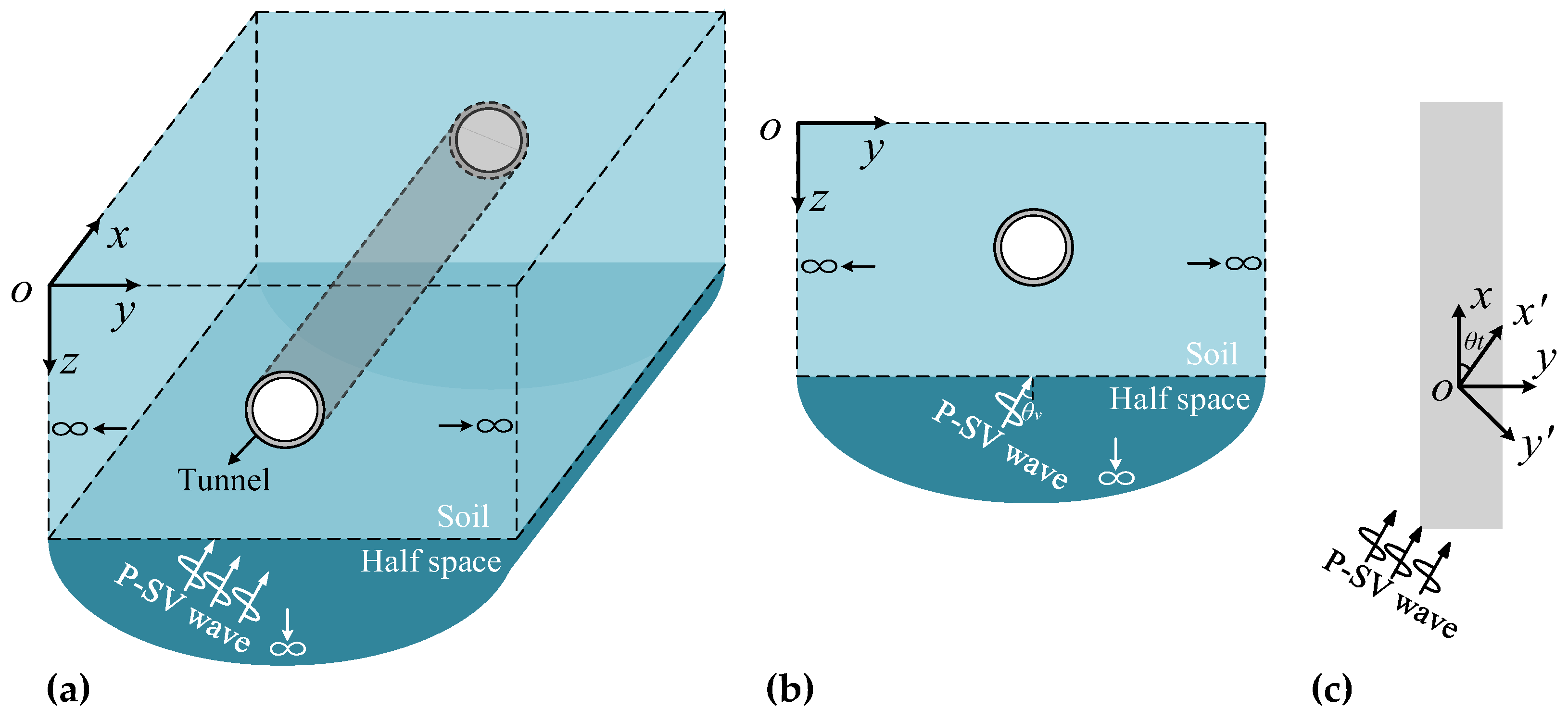
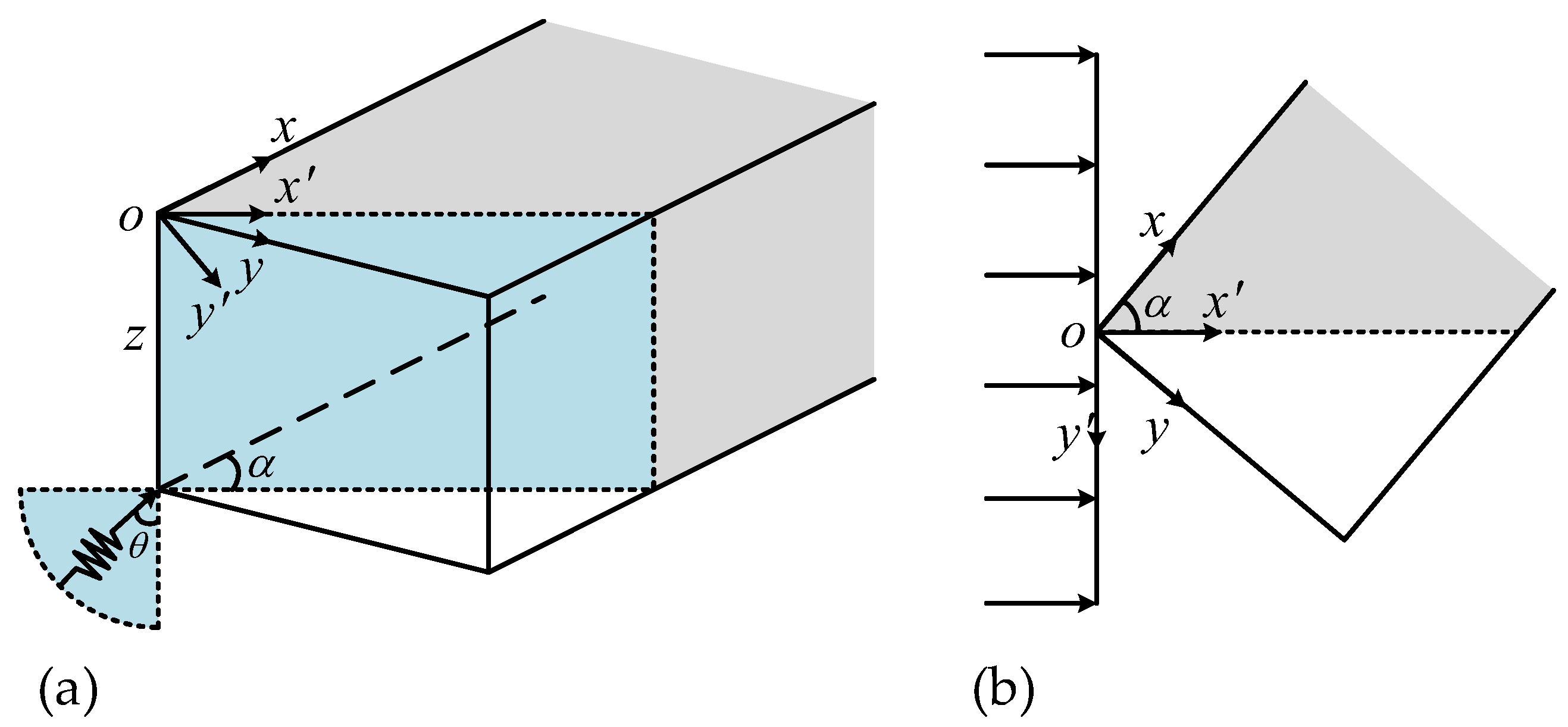
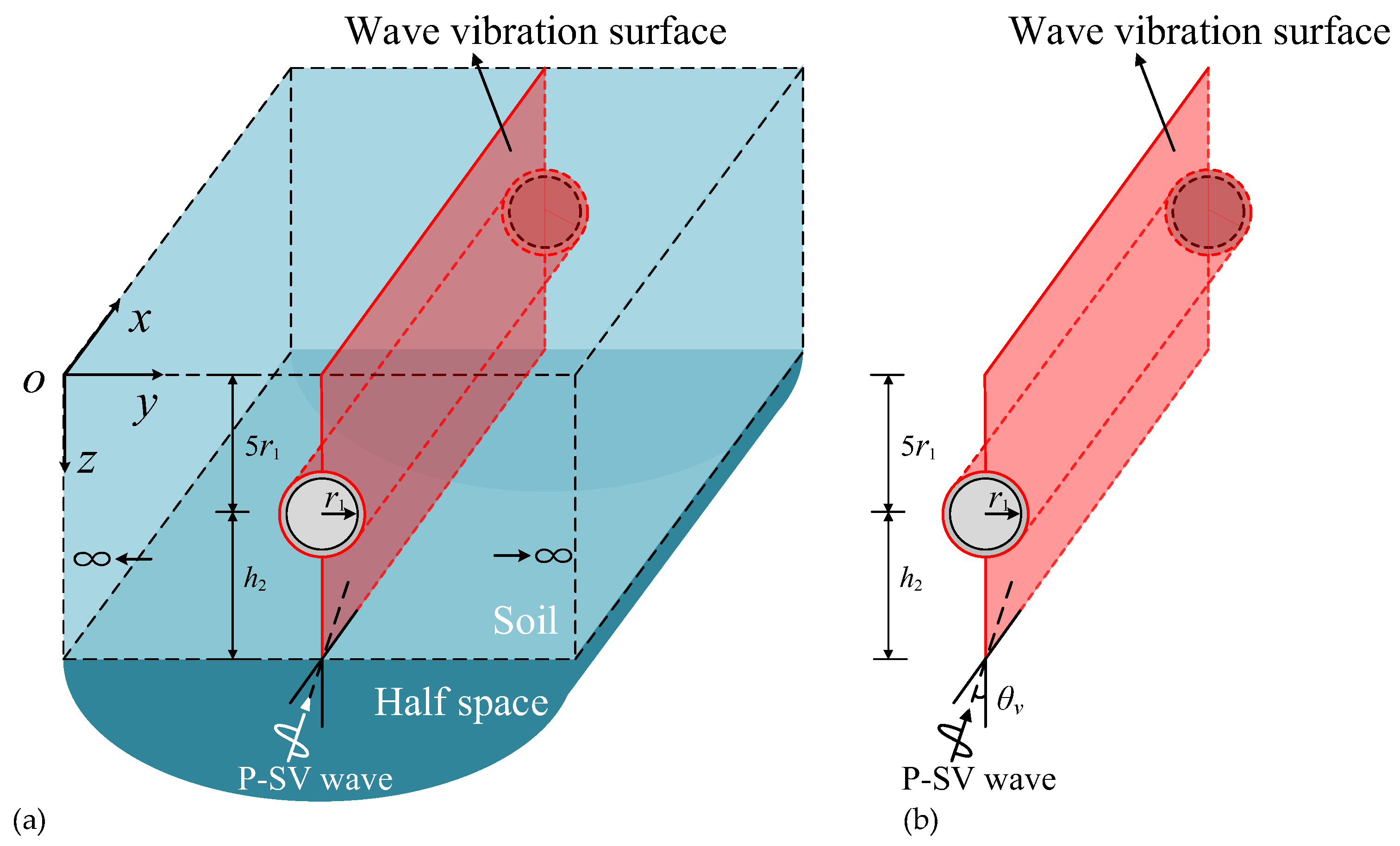
2. Wave Scattering Problem of Soil–Tunnel Interaction under Oblique Incidence of P-SV Wave

The soil–tunnel interaction system used for seismic analysis of underground long lined tunnel is shown in Figure 1a. The site is divided into the underlying half space bedrock and overlying soil layer. The interface between the soil and the tunnel is fully bonded. In addition, at the interface nodes, the displacement and stress are continuous. The geometry and material properties remain consistent along the longitudinal direction of the tunnel. The underlying half space bedrock, overlying soil layer and tunnel are assumed to be homogeneous, isotropic and linear elastic material. The surface traction and initial stress of the tunnel is zero.
In this study, the seismic wave is input from underlying half space with any angle in the form of a plane wave. The tunnel is subjected to earthquake loading by compression wave and shear wave. In the Cartesian coordinate system (x, y, z), as shown in Figure 1b, θv is defined as the incident angle between the x′ axis and the z axis. θt is the conversion angle between the x′ axis and the x axis in the x-o-y view in Figure 1c. The wave propagation direction is x′ axis.

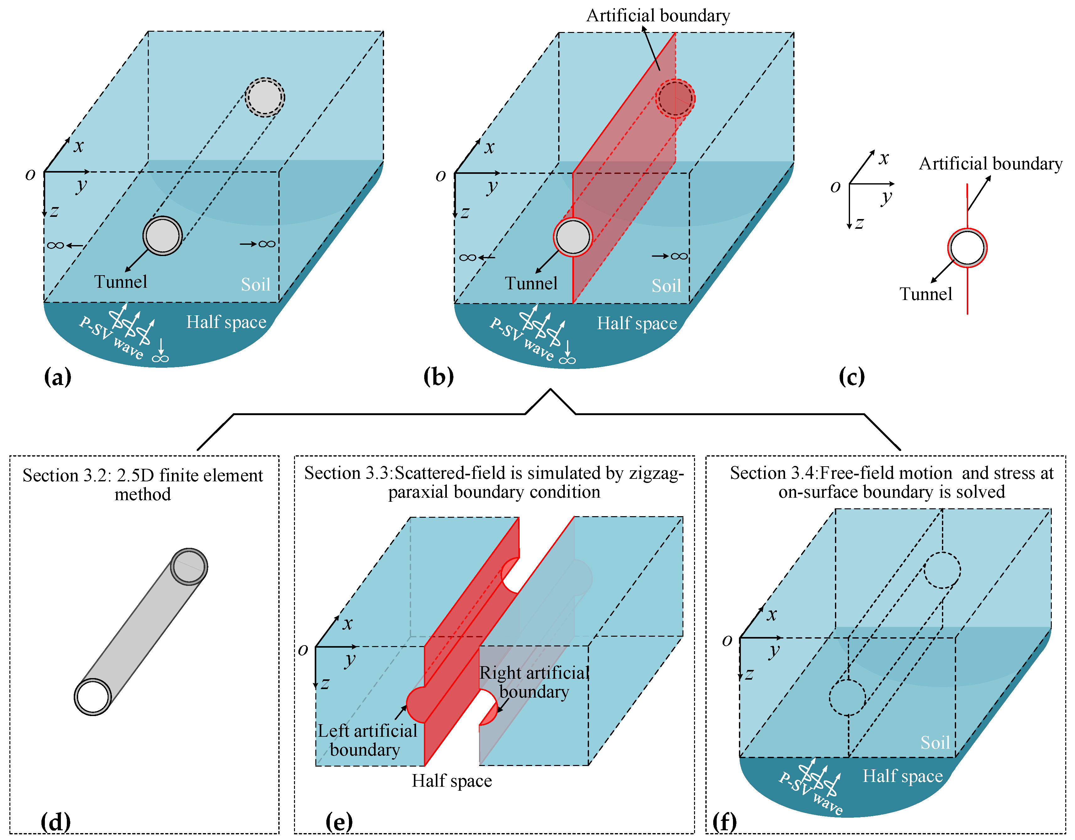
3. 2.5D Finite Element Substructure Method

3.1. The Framework of the Proposed 2.5D Finite Element Substructure Method

The framework of the 2.5D finite element substructure method is presented in Figure 2. As shown in Figure 2b, the zigzag-paraxial boundary (denoted by red surface) attached to the surface of tunnel is employed to divide the 3D model into finite domain and infinite domains. The finite domain with complex geometry and material properties is discretized based on the 2.5D finite element method in Figure 2d. The combined zigzag-paraxial boundary condition, as illustrated in Figure 2e, is presented to provide the dynamic stiffness of the truncated infinite rock or soil media and simulate scattered field. As shown in Figure 2f, wave superposition of free field and scattered field on boundary are stated, in which free field displacement and traction on the boundary are obtained by the stiffness matrix method in reference [42]. Figure 2c shows that the final total 2.5D substructure model is established.

3.2. Description of the 2.5D Finite Element Method

Through the decomposition of Figure 2b, the finite domain contains the long tunnel, which can be modeled by the 2.5D finite element method. Different from 2D finite element, each 2.5D element node has three degrees of freedom. The tunnel displacement is expressed as follows:
u ( x , y , z , t ) = N u ¯ ( y , z ) exp ( i k x x ) exp ( i ω t ) d ω
where N is the shape function matrix in the 2D isoparametric finite element analysis. The u-bar is the nodal displacement with three components in the frequency domain and wavenumber domain. i is imaginary. The circular frequency is ω. The wavenumber is given as kx = cosθvsinθtω/cb in the x direction, with cb being the wave velocity of the elastic underlying half space.
The dry soil layer is assumed to be an elastic solid medium whose governing equation can be written in global coordinate system (x, y, z) as follows:
L T σ = ω 2 ρ u ¯
where ρ is density; σ is stress matrix; L is a differential operator; the superscript T represents the transpose of the matrix; specifically, as follows:
L = [ x 0 0 y 0 z 0 y 0 x z 0 0 0 z 0 y x ] T
According to the Hooke’s law, the stress–strain relationship is
σ = D ε
where ε is strain. It is well known that D is a 3D linear elastic constitutive matrix with Lame constants λ and G.
D = [ λ + 2 G λ λ 0 0 0 λ λ + 2 G λ 0 0 0 λ λ λ + 2 G 0 0 0 0 0 0 G 0 0 0 0 0 0 G 0 0 0 0 0 0 G ]
The strain–displacement relation is
ε = B u ¯
where B is the strain matrix.
By replacing partial derivative ∂/∂x with longitudinal wave number −ikx, the calculation equation of tunnel finite element model in 2.5D form is obtained.
K u ¯ ω 2 M u ¯ = F ¯
where F ¯ is the interaction force vector between the tunnel and the surrounding soil; K and M are the stiffness matrix and mass matrix of the 2.5D tunnel model, respectively
K = B T D B J d ξ d η
M = N T ρ N J d ξ d η
where J is the Jacobian matrix which represents dξdη area mapping to dxdy.
As shown in the Figure 2d, the 2.5D finite element equation of finite domain can be rewritten as follows:
[ S p p S p q S q p S q q ] { u ¯ p u ¯ q } = { 0 F ¯ q }
with dynamic stiffness matrix
S = K ω 2 M
where subscript q represents the nodes at the interface of the soil–tunnel system and subscript p represents all structural nodes except for the structural boundary.

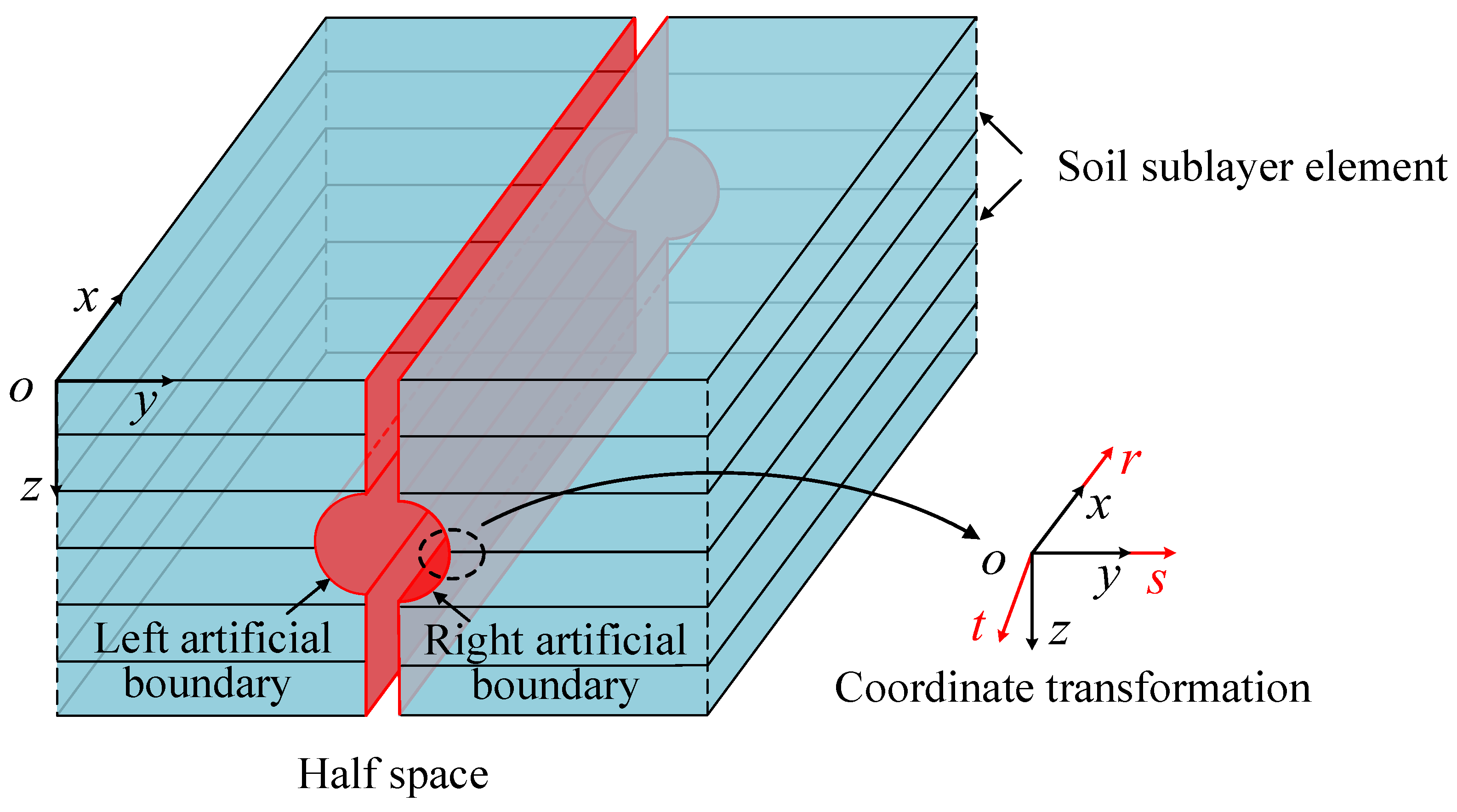
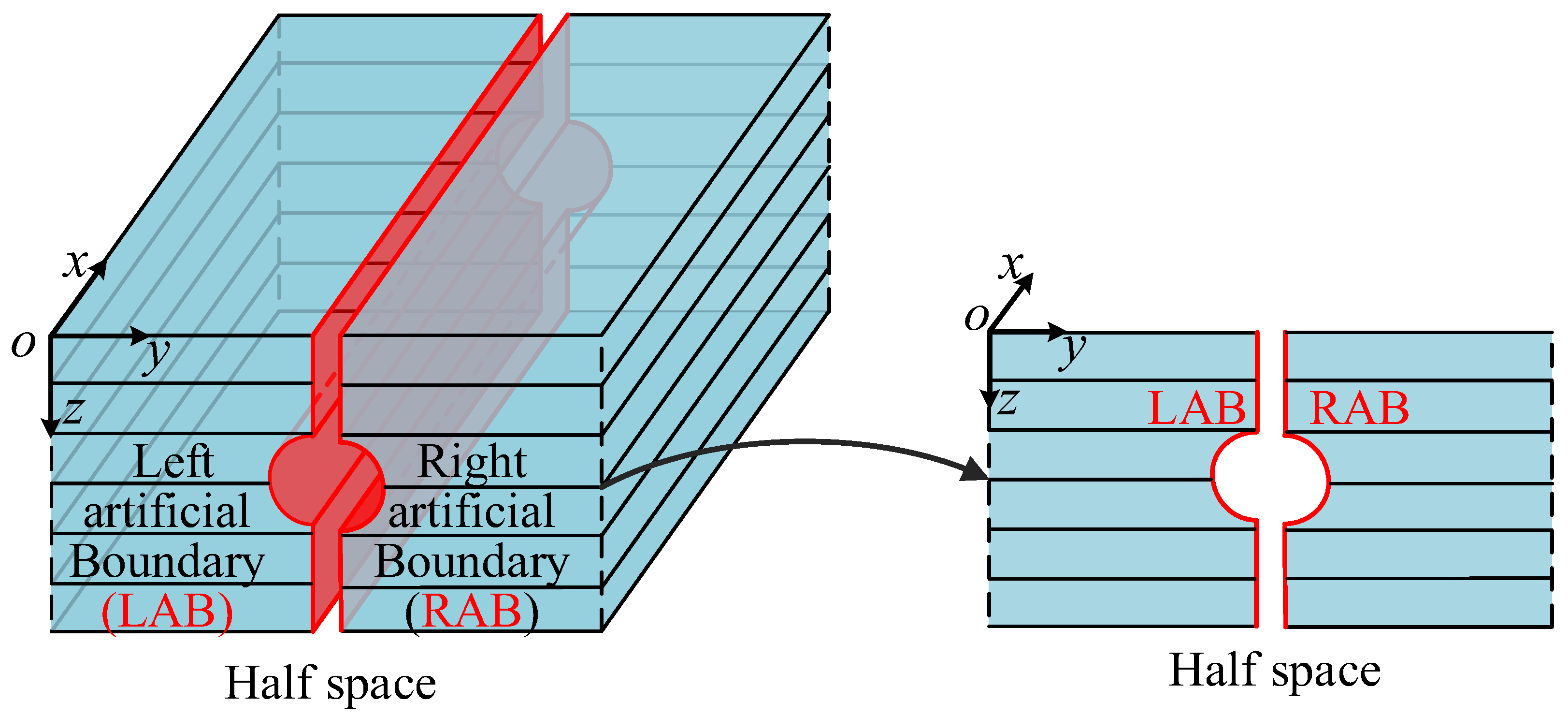
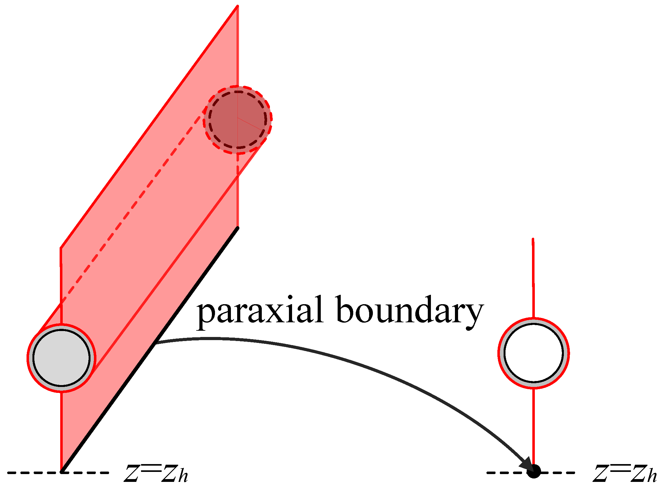
3.3. A Zigzag-Paraxial Boundary Condition Suitable for 2.5D Finite Element Method

The infinite domain includes multilayer soil and underlying half space bedrock. A zigzag-paraxial boundary condition suitable for 2.5D finite element method is presented, which can be used for efficient analysis seismic responses of long lined tunnel.
The establishment process of the 2.5D zigzag-paraxial boundary condition is introduced, leading into an independent non-orthogonal local coordinate system (r, s, t) with zigzag boundaries attached to the surface of the tunnel. Due to the artificial boundary conditions on the left and right having the same building process, the detailed derivation process of the right boundary is introduced in this subsection.
The conversion relationship between the global coordinate system (x, y, z) and the local coordinate system (r, s, t) is shown in Figure 3. The local coordinate system is used in each soil sublayer element to represent the zigzag shape of the boundary, in which the direction of r-axis and s-axis are the same as x-axis and y-axis of global coordinate, respectively. The t-axis is aligned with the zigzag shape of the surface boundary. The coordinate conversion relationship is as follows:
{ x y z } = [ 1 0 0 0 1 n y 0 0 n z ] { r s t }
where ny and nz are the y and z components of unit directional vector along t axis, respectively.
According to the Equation (12), the derivatives with respective to x, y and z can be obtained from the corresponding ones with respective to r, s and t as follows:
{ x y z } = [ 1 0 0 0 1 0 0 n y / n z 1 / n z ] { r s t }
Substituting Equation (13) into Equation (2), the wave equation of multi-layer soil can be expressed as follows:
L k T D L k u ˜ = ω 2 ρ u ˜
where the ~ on u denotes its value in frequency domain.
Since x and r have the same direction, the partial derivative along the r direction ∂/∂r is also replaced by −ikx. Lst is the differential operator in the local coordinate system. The Lst expression is as follows:
L k = [ i k x 0 0 s 0 n y n z s + 1 n z t 0 s 0 i k x n y n z s + 1 n z t 0 0 0 n y n z s + 1 n z t 0 s i k x ] T
To conveniently discretize the wave equilibrium equation along the s direction, Lk is rewritten as
L k = i k x L r + L s s + L t t
with
L r = [ 1 0 0 0 0 0 0 0 0 1 0 0 0 0 0 0 0 1 ] T
L s = 1 n z [ 0 0 0 n z 0 n y 0 n z 0 0 n y 0 0 0 n y 0 n z 0 ] T
L t = 1 n z [ 0 0 0 0 0 1 0 0 0 0 1 0 0 0 1 0 0 0 ] T
Thus, Equation (14) can be rewritten as
A s s 2 u ˜ s 2 + ( A s t + A s t T ) 2 u ˜ s t + A t t 2 u ˜ t 2 i k x [ ( A r s + A r s T ) u ˜ s + ( A r t + A r t T ) u ˜ t ] k x 2 A r r u ˜ + ω 2 ρ u ˜ = 0
with the coefficient matrices of the Equation (18) being
{ A s s = L s T D L s A s t = L s T D L t A t t = L t T D L t A r s = L r T D L s A r t = L r T D L t A r r = L r T D L r
By discretizing Equation (18) along the s direction, the displacement vector of any thin layer element can be expressed:
u ˜ = N e u ¯
with the nodal shape function matrix Ne as
N e = [ N 1 0 0 N 2 0 0 0 N 1 0 0 N 2 0 0 0 N 1 0 0 N 2 ]
with
N 1 = s 2 s s 2 s 1
N 2 = s s 1 s 2 s 1
In the frequency domain, the discrete value of displacement u ¯ at nodes are prescribed as follows:
u ¯ = { u ¯ 1 T u ¯ 2 T } T = { u 1 x u 1 y u 1 z u 2 x u 2 y u 2 z } T
Equation (20) is taken into Equation (18). The weak form of the equivalent integral is obtained by using the definition of the stress on the surface.
B s s 2 u ¯ s 2 ( B s t B s t T ) u ¯ s ( B r s + B r s T ) u ˜ s ( B r t B r t T + B r r B t t + ω 2 M ) u ¯ = σ z
with coefficient matrices of the equation
{ B s s = n z N T A s s N d t B s t = n z N T A s t N t d t B t t = n z N T t A t t N t d t B r s = i k x n z N T A r s N d t B r t = i k x n z N T A r t N t d t B r r = k x 2 n z N T A r r N d t M = ρ n z N T N d t
The stress vector on the right side of the Equation (24) can be expressed as
σ z = { n z L t T σ 1 n z L t T σ 2 } T = { τ x z τ y z σ z τ x z τ y z σ z } T
As shown in Figure 4, the zigzag boundary changes from a red surface to a curve with three degrees of freedom at each node. A zigzag boundary condition suitable for 2.5D finite element method is derived in the local coordinate system.
Due to the zigzag boundary is limited to rigid base, the 2.5D paraxial boundary condition in the underlying half space can improve the boundary accuracy. The paraxial boundary condition is a paraxial approximation of the exact dynamic stiffness matrix. When the seismic wave is incident obliquely, the relationship between the stress and the displacement at z = zh (as shown in Figure 5) on the underlying half space surface is as follows
σ ˜ h = { τ x z τ y z σ z } T = A h 2 u ˜ h y 2 B h u ˜ h y + C h u ˜ h
The matrices Ah, Bh, and Ch as the 3 × 3 matrices are given below
A h = i G h c s 2 ω [ 1 0 0 0 ( 1 2 α ) / α 3 0 0 0 ( α 2 ) / α ]
B h = [ 0 0 G h c s k x 2 ω ( α 3 2 α 2 α 3 + 1 ) 0 0 G h ( 1 2 α ) α G h c s k x 2 ω ( α 3 2 α 2 α 3 + 1 ) G h ( 1 2 α ) α 0 ]
C h = [ i ω ρ C s + i G h c s k x 2 2 ω ( α 3 2 α 2 α 3 ) i G h k x ( 1 2 α ) α 0 i G h k x ( 1 2 α ) α i ω ρ c p + i G h c s k x 2 2 ω ( 1 2 α α 3 ) 0 0 0 i ω ρ c s + i G h c s k x 2 2 ω ]
where the matrices subscript h indicates the half space; the P and SV wave velocities are cp and cs, respectively; α is the ratio of cs to cp. Gh is the shear modulus of the half-space.
The thin layer element Equation (24) is assembled by displacement and stress continuity conditions in the soil layer. According to the relationship between the global coordinate system and the local coordinate system, ∂/∂s = ∂/∂y can be obtained. Finally, combined with the relationship between the surface stress and displacement of the underlying half space Equation (27), the assembled equation of Equations (24) and (27) can be obtained
A 2 u ¯ y 2 B u ¯ y + C u ¯ = 0
with
A = B s s A h B = ( B s t B s t T + B r s + B r s T ) A h C = ( B r t + B r t T B r r + B t t ω 2 M ) C h
where the notation is used to describe 2.5D finite element assembly in the matrix.
Taking the Fourier transform of Equation (29) into the wavenumber domain and transforming into solving the quadratic eigenvalue problem,
( k y 2 A + i k y B + C ) u = = 0
where ky is the wavenumber along the y direction and u = is nodal displacement vector in the wavenumber-frequency domain.
According to Zhang et al. [44], when the seismic wave propagates in the positive direction of the y-axis, the wave number satisfies the condition that Re(ky) < 0 and Im(ky) > 0. Select the corresponding ky on the right boundary to superimpose the displacement mode as
u ¯ = Φ E y Γ
where Ey is a diagonal matrix and the diagonal elements are exp(−ikyy); Φ and Г are the eigenvector corresponding to the selected eigenvalue and the undetermined coefficient, respectively.
Taking the artificial boundary on the right as an example, the surface stress of the thin layer element is discretized. The element node stress vector can be expressed as follows
f ¯ = N T T ˜ d s = B s s u ¯ s ( B r s T + B s t ) u ¯
with the surface stress T ˜ of artificial boundary given as
T ˜ = n z L s T σ = i k x n z A r s T u ˜ n z A s s u ˜ s n z A s t u ˜ t
The force of the bedrock half space on the bottom of the overlying soil layer is represented by f ¯ h
f ¯ h = A h u ¯ h y B h 2 u ¯ h
Assembling the above f ¯ and f ¯ h , the right artificial boundary node force can be obtained
F ¯ = A u ¯ y H u ¯
with
H = B r s T + B s t + B B 2
Taking Equation (31) into Equation (35), the expression of the right boundary force-displacement relationship in the frequency-wavenumber domain is as follows
F ¯ = A Φ E y y Γ H Φ E y Γ = [ i A Φ K Φ 1 H ] Φ E y Γ = K u ¯
with
K = i A Φ K Φ 1 H
where K is a diagonal matrix consisting of diagonal elements ky and K is the stiffness coefficient of the 2.5D zigzag-paraxial boundary.
As shown in Figure 2c, a 2.5D zigzag-paraxial boundary condition be obtained, which can be written as the following
{ F ¯ l , L F ¯ c , L + F ¯ c , R F ¯ r , R } = [ K l l , L K l c , L 0 K c l , L K c c , L + K c c , R K c r , R 0 K r c , R K r r , R ] { u ¯ l u ¯ c u ¯ r }
where the subscripts L and R denote the left and right artificial boundaries, respectively; the subscripts c represent the common nodes of the left and right boundaries. The l and r only refer to the left and right boundaries of the structure.
{ F ¯ q s 0 } = [ K q q K q r K r q K r r ] { u ¯ m s u ¯ r s }
where the r represents the remaining artificial boundary nodes except the interface between soil and structure.

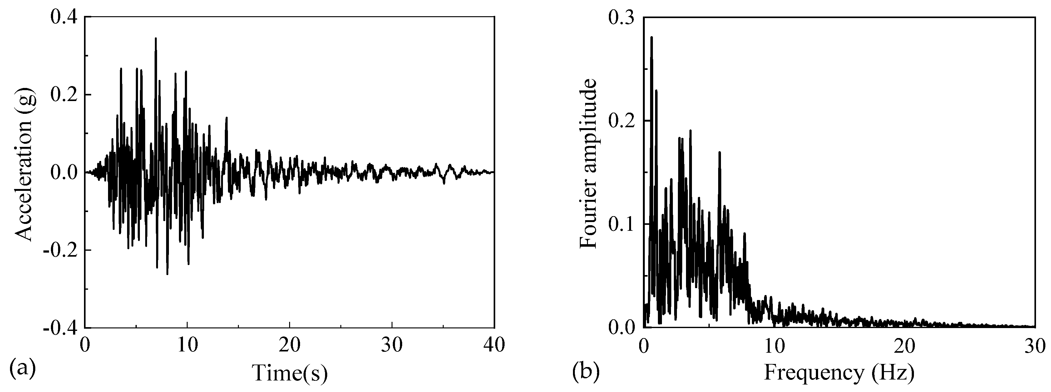
3.4. Seismic Wave Input

In this subsection, the 2.5D seismic wave input method is used to convert the incident seismic wave into the equivalent node load on the artificial boundary surface.
When solving the free field response [41], we use the stiffness matrix method [42] to calculate the free field response of the 1D site. The 3D site seismic response can be obtained through time delay. In the local coordinate system (x′, y′, z) shown in Figure 6, the displacement vector of the i-node on the artificial boundary of the soil structure interaction model can be written as
u ¯ i f ( 1 ) ( x i , y i , z i , t ) = { 0 0 t t i u ¯ j ( 0 , y i , 0 , t t i ) t > t i
with
t i = | x i cos φ + z i sin φ | c x
where the superscript (1) indicates the local coordinate system (x′, y′, z); ui and uj are the displacement of the node i and j on the 1D site response analysis; ti is the time of along the z direction from j to i.
The coordinate transformational relationship of site response on the truncated boundary is as follows
u ¯ f = Q u ¯ f ( 1 )
σ ¯ f = Q σ ¯ f ( 1 ) Q T
where u ¯ f and σ ¯ f are the displacement vector and stress vector in the global coordinates (x, y, z), respectively; the free field response is denoted by the superscript f, which is determined according to the site response. Q is the coordinate transform matrix, which can be written as
Q = [ cos α sin α 0 sin α cos α 0 0 0 1 ]
The node force of the element can be obtained from stress by finite element discretization along the boundary.
F ¯ f = L i σ ¯ f d
where d is the element outer normal vector of the artificial boundary surface; L is the element length on the 2.5D artificial boundary surface.
The scattered field response can be simulated by the proposed 2.5D zigzag-paraxial boundary conditions.

3.5. System Equation

The total force and displacement can be decomposed into the following expressions, respectively
F ¯ = F ¯ f + F ¯ s
u ¯ = u ¯ f + u ¯ s
where the scattered field, denoted by the superscript s, is unknown.
Equations (47) and (48) are brought into Equation (40). The unknown scattering field response at the artificial boundary can be represented by the known free field response and the total response.
[ K q q K q r K r q K r r ] { u ¯ q u ¯ r } = { f ¯ q f + K q q u ¯ q f + K q r u ¯ r f K r q u ¯ q f + K r r u ¯ r f }
Considering the continuous conditions of displacement and stress between layers, the 2.5D finite element Equation (10) and the 2.5D zigzag-paraxial boundary condition Equation (49) are assembled, and the equation of the 2.5D substructure method is established as follows
[ S p p S p q 0 S q p S q q + K q q K q r 0 K r q K r r ] { u ¯ p u ¯ q u ¯ r } = { 0 f ¯ q f + K q q u ¯ q f + K q r u ¯ r f K r q u ¯ q f + K r r u ¯ r f }
By inverse Fourier transform of the results, we will obtain the displacement time history of the total response of the tunnel.

4. Method Verification

The substructure models are established by using the 2.5D method combined with zigzag-paraxial boundary condition, which verifies the accuracy of the proposed method under P-SV wave incidence.

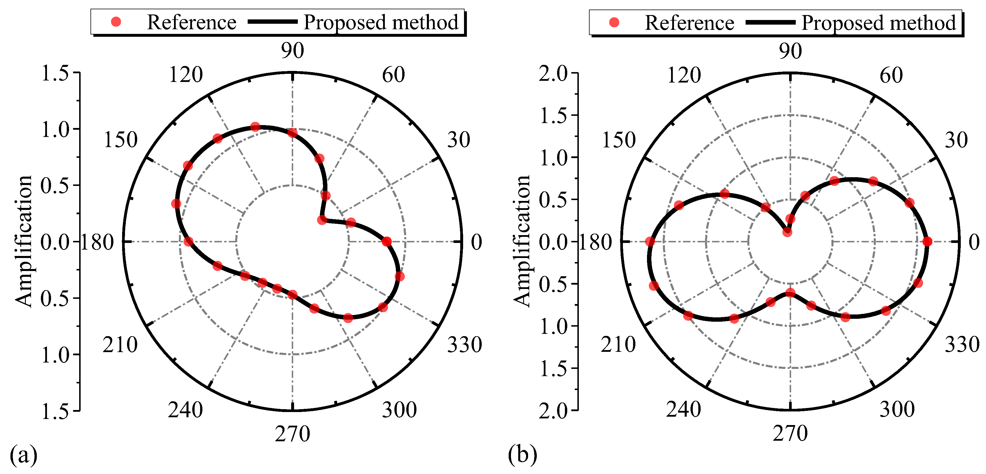
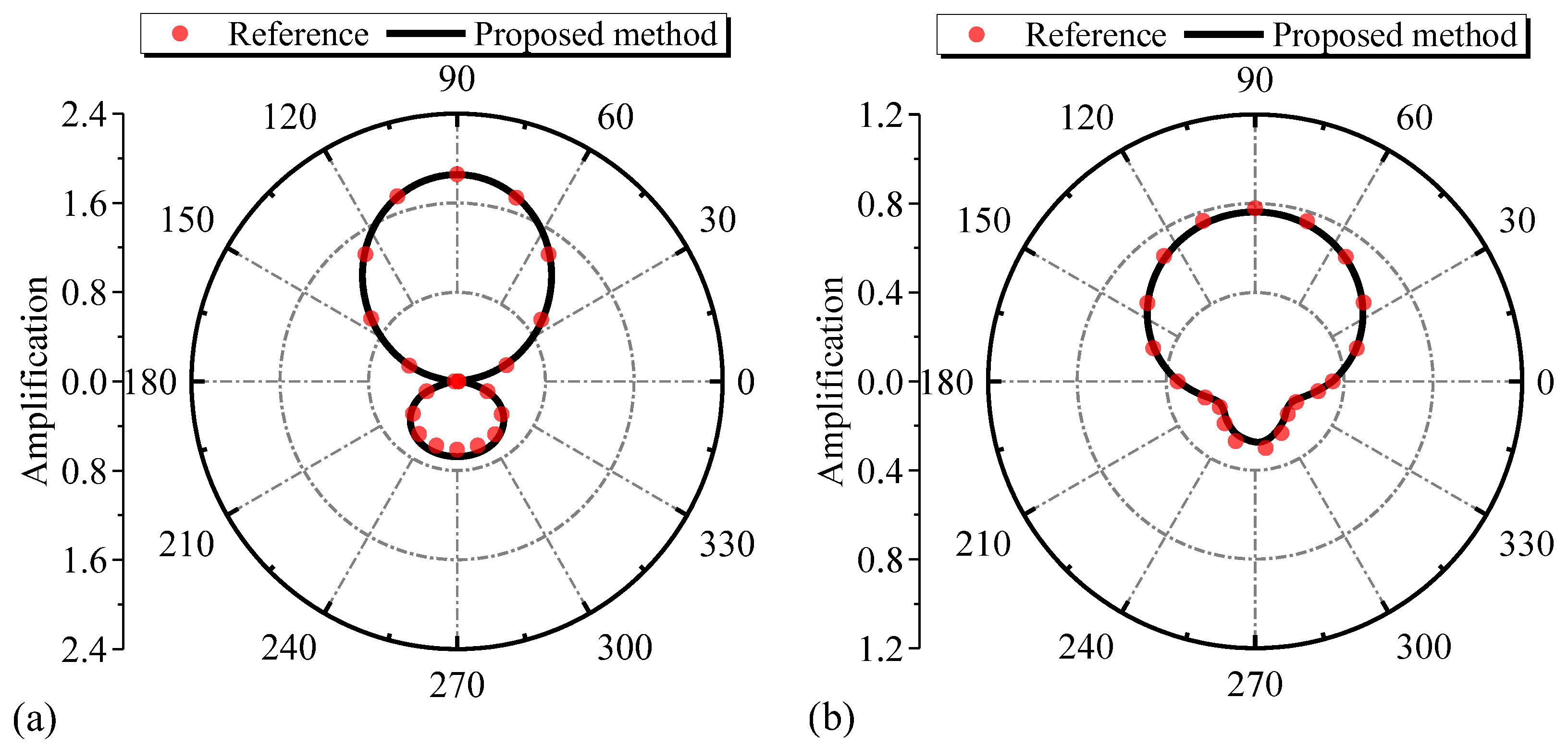
4.1. Oblique Incidence of Seismic Waves in the Plane

For the problem of P-SV wave scattering with oblique incidence at any angle in the plane, the geometric characteristics are shown in Figure 7a. The lining depth of the tunnel is H = 8.33r1, and the thickness is 0.1r1. The numerical example takes r1 = 5.0m. The material parameters are shown in Table 1. The 2.5D finite element substructure model is compared with the 2D finite domain extension model. The size of the 2D finite domain is 300 m × 140 m.
When the P wave is incident, the angle with the vertical direction is θv = 60°. For the incident SV wave, the angle with the vertical direction is θv = 15°. Due to the verification of the 2D oblique incidence problem, the conversion angle is θt = 90°. The dashed line in Figure 7a represents the 2D viscous spring artificial boundary. The radial displacement of the substructure model is compared with that of the 2D finite element model, as shown in Figure 8. It can be seen from the results that the 2.5D finite element substructure method has a high consistency with the reference solution under 2D oblique incidence.
To improve the comprehensiveness of the validation results, the data are further processed and analyzed [45]. The validation results are converted into a scatter plot based on relevant features (maximum normalized displacement amplitude for seismic simulations), as shown in Figure 9. The scatter plot uses the 3D model reference solution as the x-axis, and the 2.5D model solution is used as the y-axis.
Based on validation example 4.1, the R2, maximum error, average error and standard deviation of the correlation coefficient kc are calculated. The results are listed in Table 2. It can be seen from Table 2 that all R2 values are close to 1, indicating that the 2.5D substructure method proposed in the paper is consistent with the 3D reference solution.

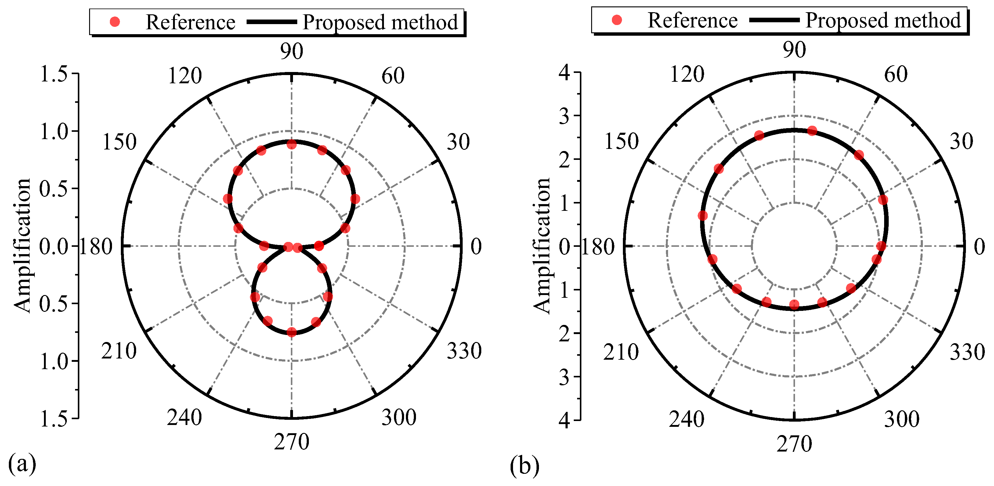
4.2. Incidence along the Longitudinal Direction

For the accuracy of the longitudinal response of the method proposed, according to the results proposed by Debarros and Luco [46], the P-SV waves incident obliquely along the tunnel axis were analyzed. The substructure model is shown in Figure 10b; the oblique incidence angle θv = 30° and the conversion angle θt = 0° of the seismic wave are input. The corresponding dimensionless frequency is η = ωr1/πcs. Tunnel are buried with a depth of H = 5.0r1 = 4.545r0 and a lining thickness of d = 0.1r1 = 0.0909r0. The material parameters are shown in Table 3.
By comparing the normalized radial displacement ur(r0) in Figure 11 and the normalized longitudinal displacement ul(r0) in Figure 12, the longitudinal seismic response of the 2.5D finite element substructure calculation method is highly in agreement with the reference solution.
Figure 13 and Figure 14 show the comparison between the 2.5D calculated value and the 3D reference solution for each node when seismic waves are obliquely incident along the longitudinal direction. The closer the data points are to the 1:1 line, the more accurate the proposed method out of the plane.
It can be seen from Table 4 that all R2 values are close to 1, indicating that the 2.5D substructure method proposed in the paper is consistent with the 3D reference solution. On the whole, the statistical indicators used for evaluation show that the 2.5D model proposed in this article has high accuracy.

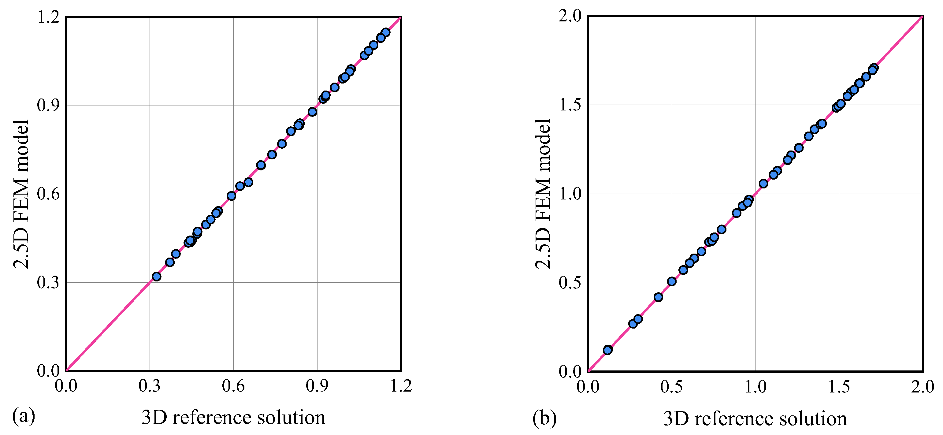
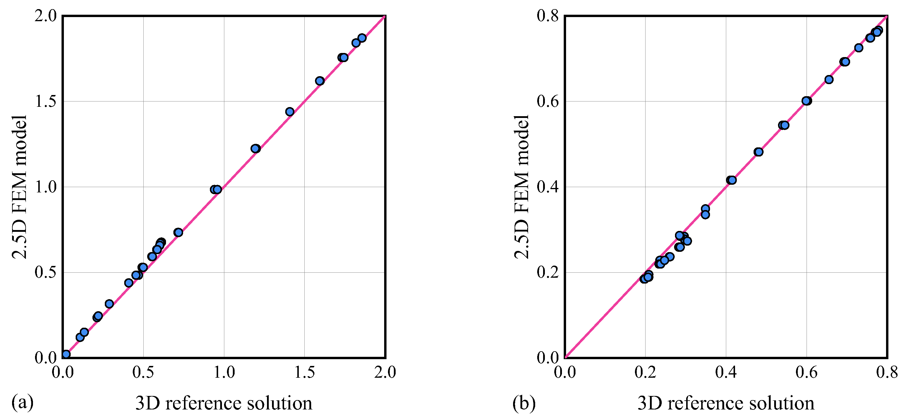
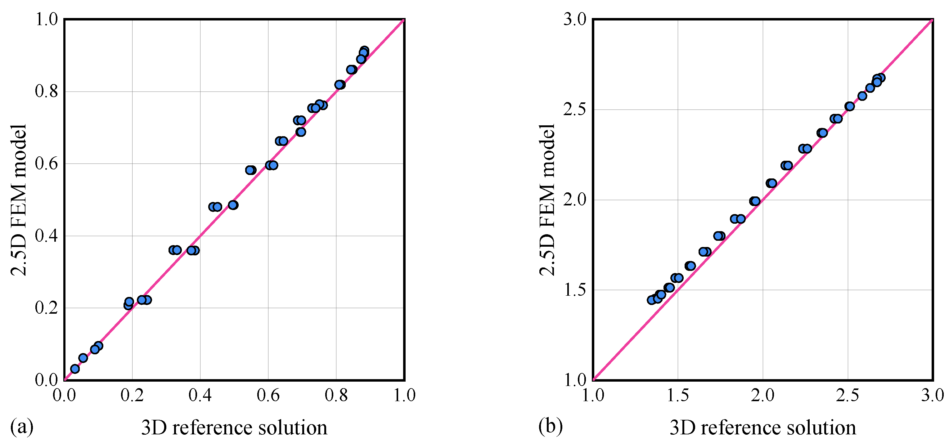
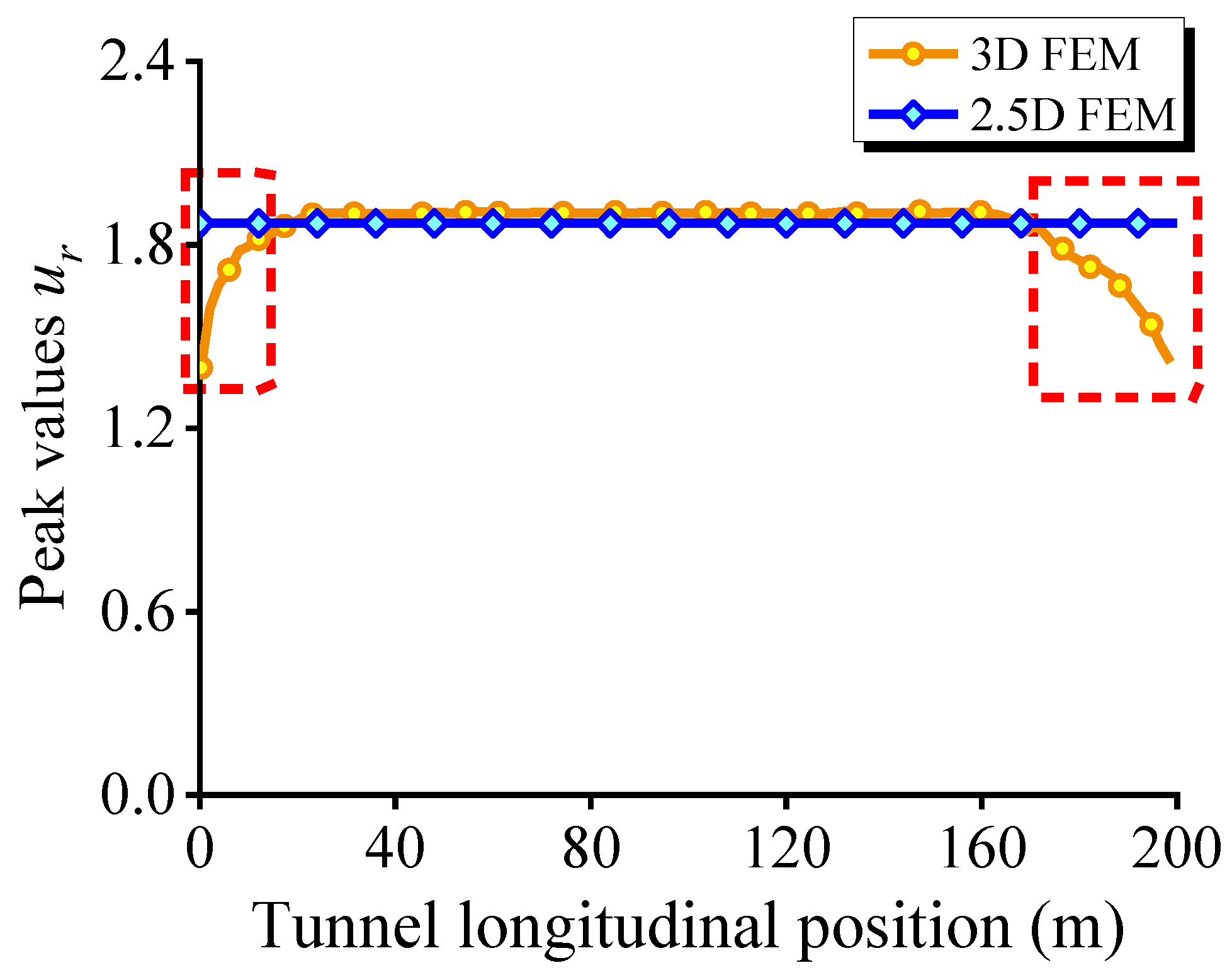
4.3. Accuracy of Longitudinal Responses

According to the 3D finite element calculation model established by Huang et al. [13], the length, width and height are 220 m, 60 m and 80 m, respectively. The length of the tunnel is 200 m. In the middle section of the numerical model, the response of the tunnel is accurate and is not affected by the truncation of both sides. The calculated material parameters are the same as Table 3. The 2.5D substructure method proposed in this paper is verified with a numerical example of the 3D finite element method. The substructure model and the incident angle of seismic wave are the same as those in Section 4.2.
Figure 15 shows the peak value of radial displacement ur along the longitudinal direction of 3D tunnel finite element model and 2.5D tunnel finite element model respectively. In fact, when seismic motion is incident on the underlying half space at any incident angle, according to Snell’s law of wave propagation, the seismic peak response along the longitudinal direction of the tunnel is the same. There is only a delay of occurred time of dynamic response, so the peak value should be constant along the longitudinal direction of the tunnel, as shown in the 2.5D finite element method results presented in Figure 15. In the middle section of the tunnel, the seismic response results of the two methods are basically consistent. The two sides of the 3D long tunnel model are truncated, resulting in the error of the numerical calculation results (as shown by the red dashed box in Figure 15). It is found that the 2.5D finite element model can avoid the disturbance caused by the truncation of the tunnel in the longitudinal direction. At the same time, compared with the calculation time of 3D finite element model, the time cost of using 2.5D substructure model is only 1/6, which reflects the efficiency of 2.5D substructure calculation method.

5. P-SV Wave Scattering of Long Lined Tunnel

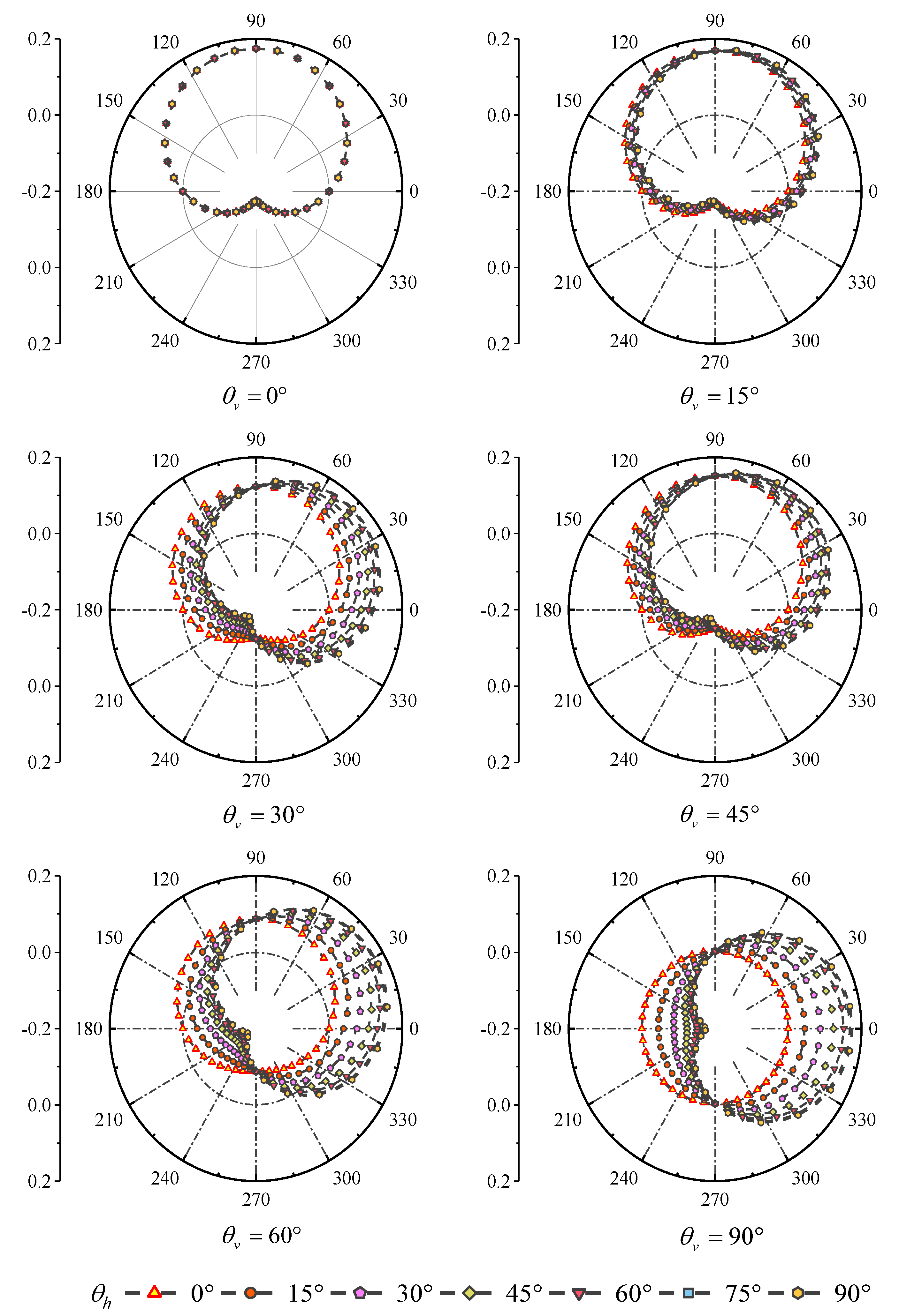
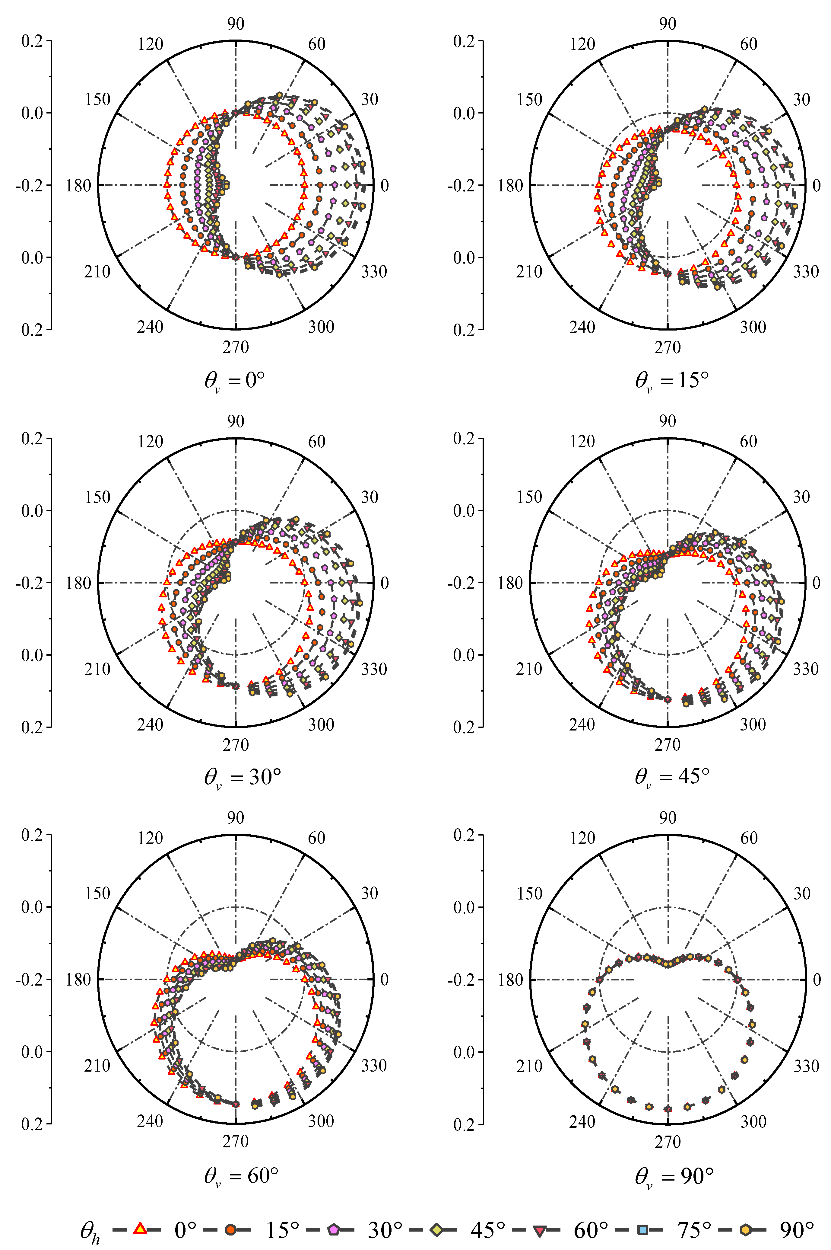
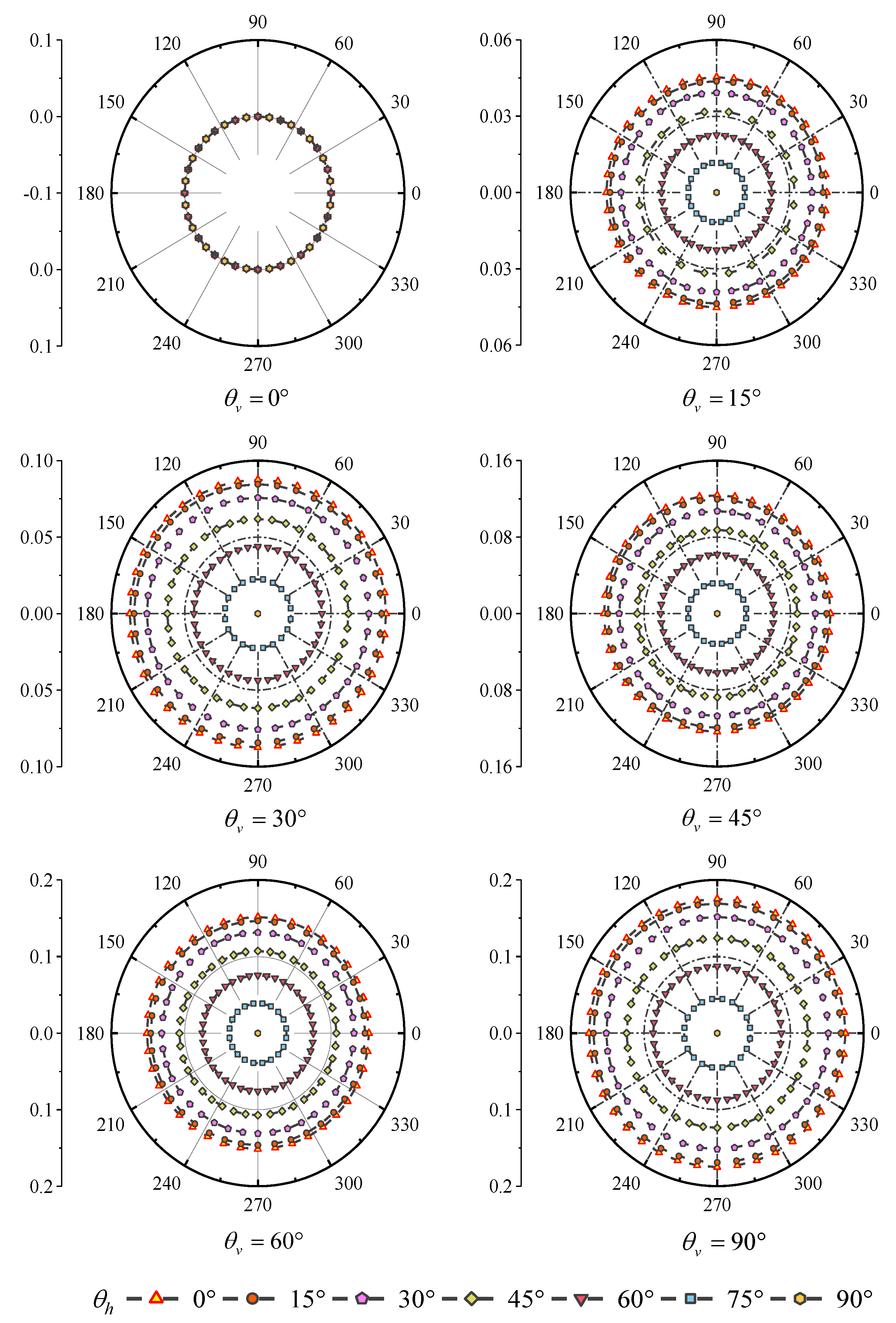
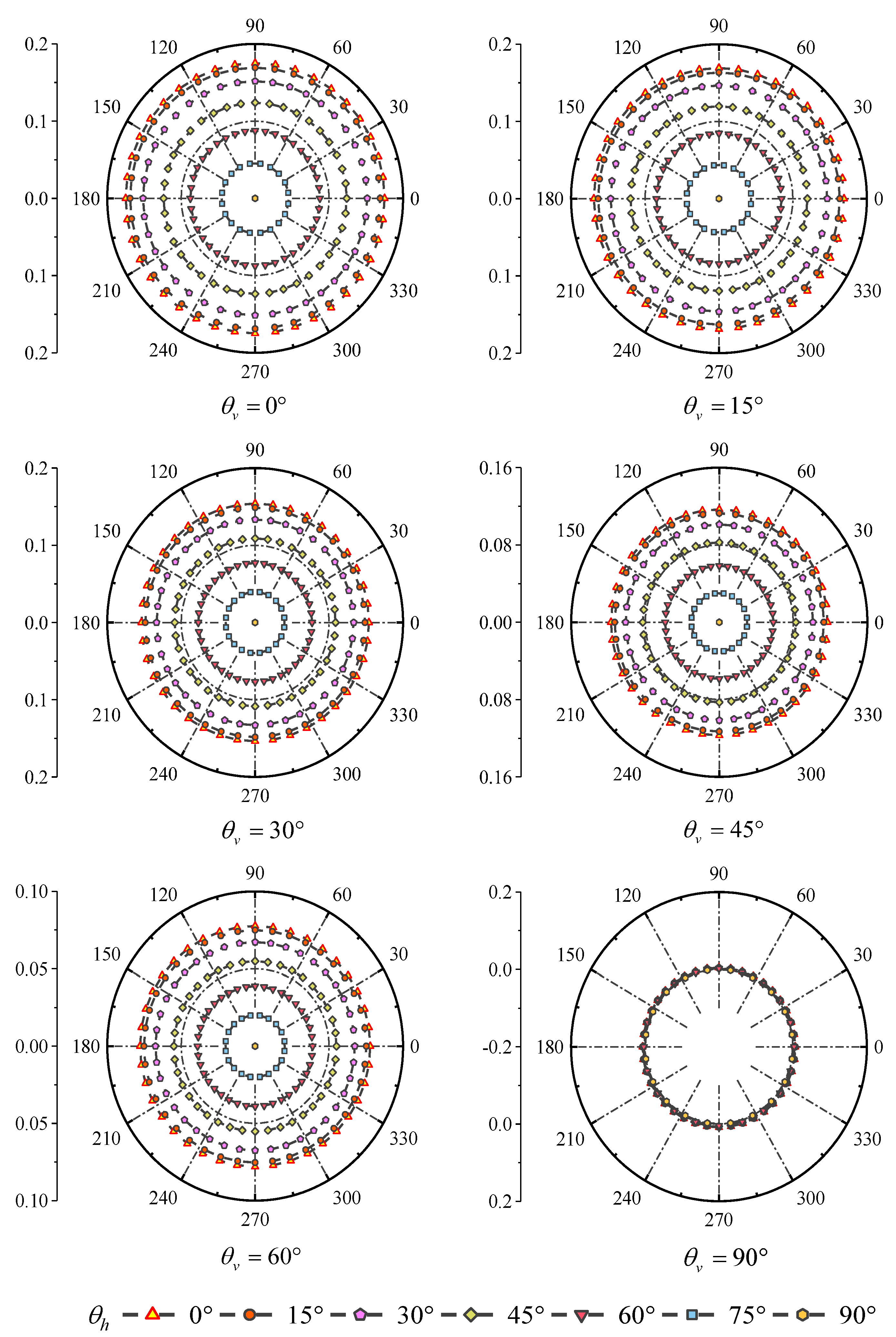
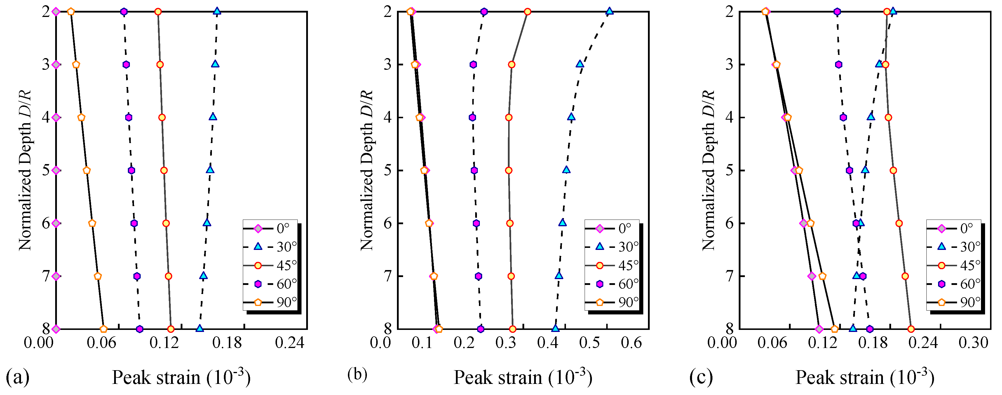
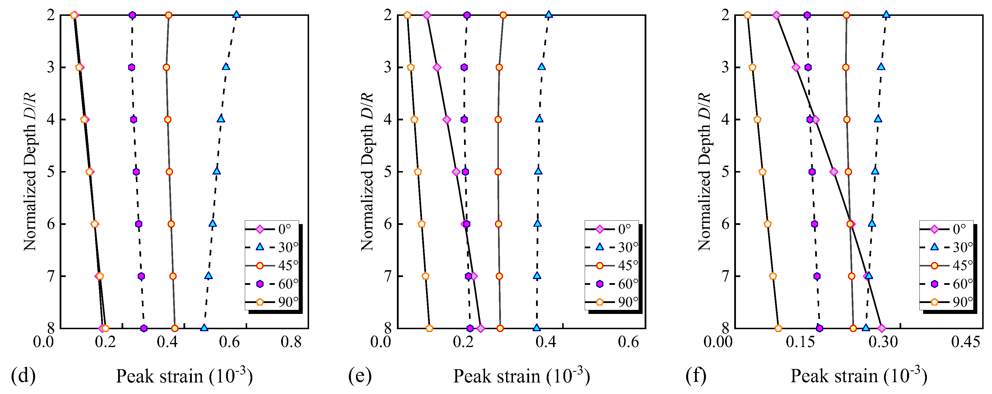
5.1. Influence of Seismic Wave Incidence Angle and Conversion Angle on Seismic Response of Tunnels

The computational model is shown in Figure 16. The tunnel and site parameters are shown in Table 1. Kobe wave is selected for the incident seismic wave record. The acceleration time history curve and spectrum curve are shown in Figure 17. For the incident with the P wave and the SV wave, respectively, the incident angle θv ranges from 0° to 90°, and the conversion angle θt ranges from 0° to 90°. The increment interval between the incident angle and the conversion angle is 15°. The external surface seismic responses of tunnel lining are calculated under different incident angles and conversion angles.
At dimensionless frequency η = 0.132, Figure 18 shows the variation of radial displacement when the P wave is incident at different incident angles and conversion angles. With the gradual increase of the incident angle, the position of the maximum radial displacement gradually shifted from the vault to the haunch. Except for vertical incidence, for the same incidence angle, the radial displacement of the tunnel lining increases gradually with the increase of the conversion angle. The radial displacement values of the SV wave at different incident angles are given in Figure 19. At this time, with the increase of the incident angle, the position of the maximum radial displacement is gradually shifted from the haunch to the arch bottom. For the axial displacement, Figure 20 shows that when the P wave is incident and the conversion angle is fixed, the axial displacement increases gradually with the increase of the incident angle. In the case of the same incident angle, the larger the conversion angle, the smaller the radial displacement. When the SV wave is incident and the conversion angle remains the same, as the angle of incidence increases, the radial displacement decreases gradually in Figure 21. Therefore, when the incident angle is large, the longitudinal seismic response of the tunnel should be given enough attention. With the change of the transfer angle, the position of the maximum seismic response of the tunnel in the cross section is changed.

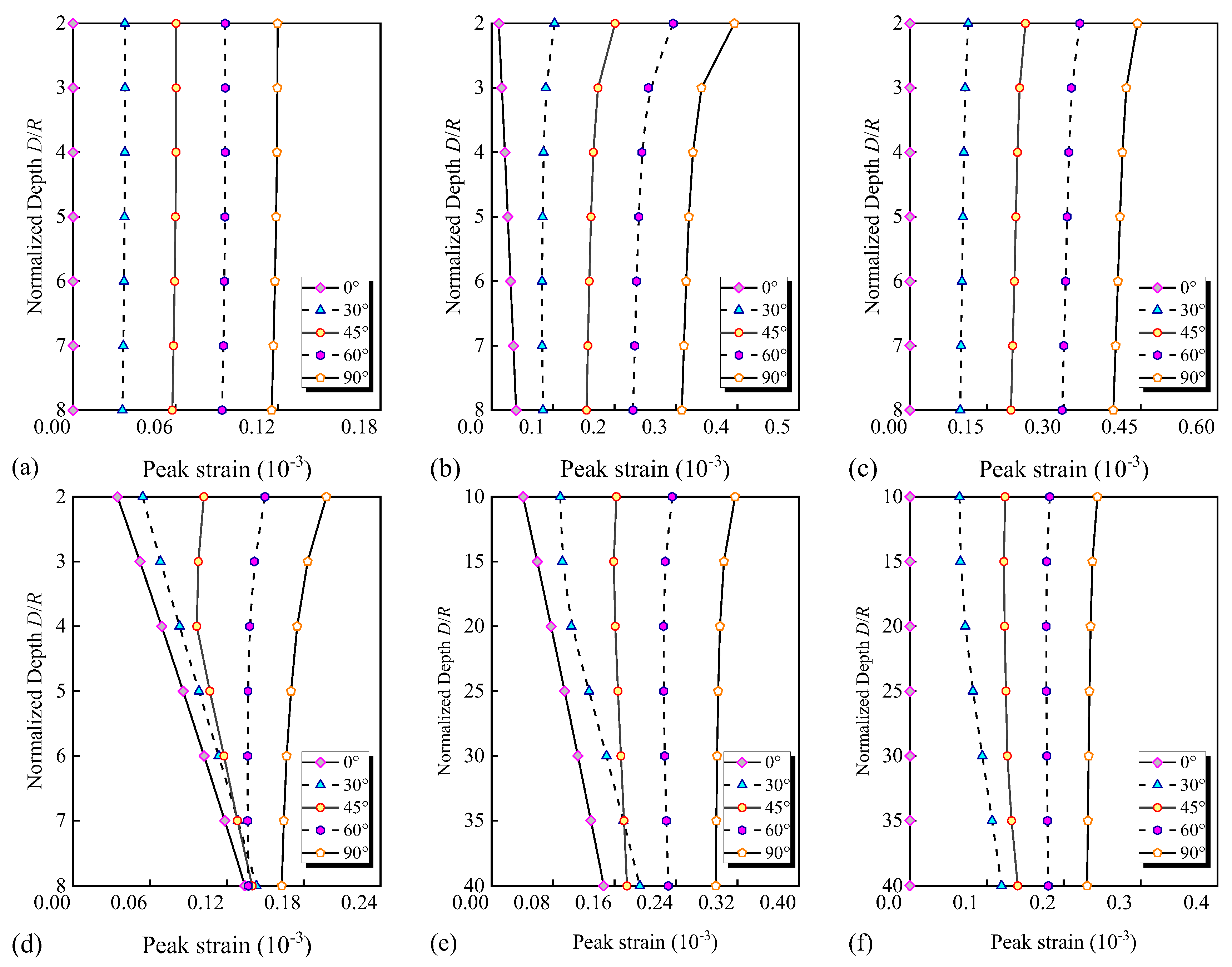
5.2. Influence of Buried Depths of Tunnels

The parameters and dimensions of tunnel material, thickness of soil layer and seismic waves selected for ground motion input are the same as those in Section 5.1, and the parameters of site and bedrock are shown in Table 3. The depth of the tunnel center is 10~40 m. According to the shear wave velocity of the medium and the dominant frequency of the seismic wave, the mesh size of the finite element is determined. The seismic wave is obliquely incident on the bedrock surface. According to the discussion in Section 5.1, the fixed conversion angle is 45° and the oblique incidence inclination angle is changed. The seismic response law of the tunnel lining at different burial depths and the influence of the change of the oblique incident angle on the seismic response of the lining at the same burial depth were investigated. To ensure the generalization, normalized depth is the ratio of tunnel burial depth D to inner diameter R, which is used to describe the influence of the embedded depth.
Figure 22 and Figure 23 show the maximum values of normal strain and shear strain of the tunnel lining under the incidence of P wave and SV wave, respectively. As can be seen from Figure 22a–c, when the P wave is incident, as the distance from the center point of the tunnel to the surface gradually increases, the normal strains in the three directions gradually decrease in most calculated conditions; this illustrates that the seismic response of the shallow buried structure cannot be ignored. The shear strain increases with the burial depth at a small incident angle (less than 45°). When the incident angle is larger, the shear strain decreases with the increase of burial depth. SV wave results are given in Figure 23.
As the burial depth increases, the internal force of the tunnel will gradually decrease. Figure 24 shows the time history curves of the maximum internal force calculated from the burial depth of 10 m when the P wave and SV wave are incident, respectively.

6. Conclusions

In this study, combined with 2.5D finite element method, zigzag-paraxial boundary condition and seismic wave input method, a 2.5D substructure method for analyzing wave scattering of tunnel in half space is proposed. Compared with the 3D time history analysis, the computational efficiency is greatly improved by using the 2.5D finite element substructure method. It provides a high efficiency analysis method for calculating large-scale seismic response of long linear underground structures.
The high precision artificial boundary condition can be placed on the surface of the structure, which greatly saves the computational cost. The dynamic stiffness of the surrounding infinite domain is provided. Under the incident P-SV wave, the proposed method is compared with the numerical model and the analytical solution. The correctness of the uniform half space wave scattering problem is verified by the calculation results. Further comparison shows that the 2.5D substructure method can effectively avoid the disturbance caused by the truncation of the tunnel in the longitudinal direction. In order to verify the capability of the proposed method, the actual seismic records are used in the numerical examples. When the P-SV wave is incident, the influence law of the incident angle of the seismic wave is mainly discussed. The effect of burial depth on the seismic response of lining structures is presented.
At the same time, the proposed method can also adapt to the complex structural shape of the cross section and the multi-structure soil–structure interaction problem. Due to the high precision of this method, discussing the changes of different model factors can provide accurate analysis for engineering design. The dynamic stiffness matrix of the underlying half space is obtained by the second-order paraxial approximation. In the next work, researchers can provide a new way to further improve the accuracy of the paraxial boundary.

Author Contributions

Conceptualization, Q.Z. and X.D.; methodology, Q.Z., M.Z. and J.H.; software, Q.Z.; validation, Q.Z. and J.H.; data curation, J.H.; writing—original draft preparation, Q.Z. and J.H.; writing—review and editing, M.Z.; visualization, G.Z.; supervision, X.D.; project administration, X.D. All authors have read and agreed to the published version of the manuscript.

Funding

This work described in this paper is supported by the National Natural Science Foundation of China (52278476 and 52208484), Project funded by China Postdoctoral Science Foundation (2022M721882) and National Key Research and Development Program (2022YFC3003603, 2022YFC3004304), which are gratefully acknowledged.

Institutional Review Board Statement

Not applicable.

Informed Consent Statement

Not applicable.

Data Availability Statement

The relevant data are all included in the paper.

Conflicts of Interest

The authors declare no conflict of interest.

References

  1. Iida, H.; Hiroto, T.; Yoshida, N.; Lwafuji, M. Damage to Daikai subway station. Soils Found 1996, 36, 283–300. [Google Scholar] [CrossRef] [PubMed]
  2. Stamo, A.A.; Beskos, D.E. Dynamic analysis of large 3-D underground structures by the BEM. Earthq. Eng. Struct. Dyn. 1995, 24, 917–934. [Google Scholar] [CrossRef]
  3. Stamos, A.A.; Beskos, D.E. 3-D seismic response analysis of long lined tunnels in half-space. Soil Dyn. Earthq. Eng. 1996, 15, 111–118. [Google Scholar] [CrossRef]
  4. Huo, H.; Bobet, A.; Fernández, G.; Fernandez, G.; Ramirez, J. Load transfer mechanisms between underground structure and surrounding ground: Evaluation of the failure of the Daikai station. J. Geotech. Geoenviron. Eng. 2005, 131, 1522–1533. [Google Scholar] [CrossRef]
  5. Hashash, Y.M.A.; Hook, J.J.; Schmidt, B.; Yao, J.I. Seismic design and analysis of underground structures. Tunn. Undergr. Space Technol. 2001, 16, 247–293. [Google Scholar] [CrossRef]
  6. Owen, G.N.; Scholl, R.E. Earthquake Engineering of Large Underground Structures; Federal Highway Administration: Washington, DC, USA, 1981. [Google Scholar]
  7. Yu, H.T.; Cai, C.; Yuan, Y.; Jia, M.C. Analytical solutions for Euler-Bernoulli Beam on Pasternak foundation subjected to arbitrary dynamic loads. Int. J. Numer. Anal. Methods Geomech. 2017, 41, 1125–1137. [Google Scholar] [CrossRef]
  8. John, C.; Zahrah, T.F. Aseismic design of underground structures. Tunn. Undergr. Space Technol. 1987, 2, 165–197. [Google Scholar] [CrossRef]
  9. Chen, J.; Shi, X.; Li, J. Shaking table test of utility tunnel under non-uniform earthquake wave excitation. Soil Dyn. Earthq. Eng. 2010, 30, 1400–1416. [Google Scholar] [CrossRef]
  10. Yu, H.T.; Yuan, Y.; Qiao, Z.Z.; Gu, Y.; Yang, Z.H.; Li, X.D. Seismic analysis of a long tunnel based on multi664 scale method. Eng. Struct. 2013, 49, 572–587. [Google Scholar] [CrossRef]
  11. Li, P.; Song, E.X. Three-dimensional numerical analysis for the longitudinal seismic response of tunnels under an asynchronous wave input. Comput. Geotech. 2015, 63, 229–243. [Google Scholar] [CrossRef]
  12. Fabozzi, S.; Bilotta, E.; Yu, H.T.; Yuan, Y. Effects of the asynchronism of ground motion on the longitudinal behaviour of a circular tunnel. Tunn. Undergr. Space Technol. 2018, 82, 529–541. [Google Scholar] [CrossRef]
  13. Huang, J.Q.; Du, X.L.; Jin, L.; Zhao, M. Impact of incident angles of P waves on the dynamic responses of long lined tunnels. Earthq. Eng. Struct. Dyn. 2016, 45, 2435–2454. [Google Scholar] [CrossRef]
  14. Gao, Z.D.; Zhao, M.; Huang, J.Q.; Du, X.L. Three-dimensional nonlinear seismic response analysis of subway station crossing longitudinally inhomogeneous geology under obliquely incident P waves. Eng. Geol. 2021, 293, 106341. [Google Scholar] [CrossRef]
  15. Miao, Y.; Yao, E.L.; Ruan, B.; Zhuang, H.Y. Seismic response of shield tunnel subjected to spatially varying earthquake ground motions. Tunn. Undergr. Space Technol. 2018, 77, 216–226. [Google Scholar] [CrossRef]
  16. Hwang, R.; Lysmer, J. Response of buried structures to traveling waves. J. Geotech. Geoenviron. 1981, 107, 183–200. [Google Scholar] [CrossRef]
  17. Yang, Y.B.; Hung, H.H. A 2.5D finite/infinite element approach for modelling viscoelastic bodies subjected to moving loads. Int. Int. J. Numer. Anal. Methods Geomech. 2001, 51, 1317–1336. [Google Scholar] [CrossRef]
  18. Alves, C.P.; Calçada, R.; Silva, C.A.; Bodare, A. Influence of soil non-linearity on the dynamic response of high-speed railway tracks. Soil Dyn. Earthq. Eng. 2010, 30, 221–235. [Google Scholar] [CrossRef]
  19. Sheng, X.; Jones, C.J.C.; Thompson, D.J. Prediction of ground vibration from trains using the wavenumber finite and boundary element methods. J. Sound Vibr. 2006, 293, 575–586. [Google Scholar] [CrossRef]
  20. François, S.; Schevenels, M.; Galvín, P.; Lombaert, G.; Degrande, G. A 2.5D coupled FE-BE methodology for the dynamic interaction between longitudinally invariant structures and a layered halfspace. Comput. Meth. Appl. Mech. Eng. 2010, 199, 1536–1548. [Google Scholar] [CrossRef]
  21. He, C.; Zhou, S.; Di, H.; Shan, Y. A 2.5-D coupled FE-BE model for the dynamic interaction between saturated soil and longitudinally invariant structures. Comput. Geotech. 2017, 82, 211–222. [Google Scholar] [CrossRef]
  22. Jin, Q.; Thompson, D.J.; Lurcock, D.; Toward, M.; Ntotsios, E. A 2.5D finite element and boundary element model for the ground vibration from trains in tunnels and validation using measurement data. J. Sound Vibr. 2018, 422, 373–389. [Google Scholar] [CrossRef]
  23. Lopes, P.; Alves Costa, P.; Calçada, R.; Silva Cardoso, A.; Costa, P.A.; Calçada, R.; Cardoso, A.S. Influence of soil stiffness on building vibrations due to railway traffic in tunnels: Numerical study. Comput. Geotech. 2014, 61, 277–291. [Google Scholar] [CrossRef]
  24. Rieckh, G.; Kreuzer, W.; Waubke, H.; Balazs, P. A 2.5D-Fourier-BEM model for vibrations in a tunnel running through layered anisotropic soil. Eng. Anal. Bound. Elem. 2012, 36, 960–967. [Google Scholar] [CrossRef]
  25. Liravi, H.; Arcos, R.; Clot, A.; Conto, F.; Romeu, J. A 2.5D coupled FEM–SBM methodology for soil–structure dynamic interaction problems. Eng. Struct. 2021, 250, 113371. [Google Scholar] [CrossRef]
  26. Lin, K.C.; Hung, H.H.; Yang, J.P.; Yang, Y.B. Seismic analysis of underground tunnels by the 2.5D finite/infinite element approach. Soil Dyn. Earthq. Eng. 2016, 85, 31–43. [Google Scholar] [CrossRef]
  27. Zhu, J.; Liang, J.W.; Ba, Z.N. A 2.5D equivalent linear model for longitudinal seismic analysis of tunnels in water-saturated poroelastic half-space. Comput. Geotech. 2019, 109, 166–188. [Google Scholar] [CrossRef]
  28. Zhu, J.; Li, X.J.; Liang, J.W. 2.5D FE-BE modelling of dynamic responses of segmented tunnels subjected to obliquely incident seismic waves. Soil Dyn. Earthq. Eng. 2022, 163, 107564. [Google Scholar] [CrossRef]
  29. Zhu, J.; Li, X.; Liang, J. 3D seismic responses of a long lined tunnel in layered poro-viscoelastic half-space by a hybrid FE-BE method. Eng. Anal. Bound. Elem. 2020, 114, 94–113. [Google Scholar] [CrossRef]
  30. Du, X.L.; Zhao, M. Stability and identiffcation for rational approximation of frequency response function of unbounded soil. Earthq. Eng. Struct. Dyn. 2010, 39, 165–186. [Google Scholar]
  31. Zhao, M.; Wu, L.H.; Du, X.L.; Zhong, Z.L.; Xu, C.S.; Li, L. Stable high-order absorbing boundary condition based on new continued fraction for scalar wave propagation in unbounded multilayer media. Comput. Meth. Appl. Mech. Eng. 2018, 334, 111–137. [Google Scholar] [CrossRef]
  32. Mossessian, T.K.; Dravinski, M. Application of a hybrid method for scattering of P, SV, and Rayleigh waves by near-surface irregularities. Bull. Seismol. Soc. Amer. 1987, 77, 1784–1803. [Google Scholar]
  33. Mojtabazadeh-Hasanlouei, S.; Panji, M.; Kamalian, M. Attenuated orthotropic time-domain half-space BEM for SH-wave scattering problems. Geophys. J. Int. 2022, 229, 1881–1913. [Google Scholar] [CrossRef]
  34. Panji, M.; Mojtabazadeh-Hasanlouei, S. On subsurface box-shaped lined tunnel under incident SH-wave propagation. Front. Struct. Civ. Eng. 2021, 15, 948–960. [Google Scholar] [CrossRef]
  35. Panji, M.; Mojtabazadeh Hasanlouei, S. Time-history response on the surface by regularly distributed enormous embedded cavity: Incident SH-waves. Earthq. Sci. 2018, 31, 137–153. [Google Scholar] [CrossRef]
  36. Shah, A.H.; Wong, K.C.; Datta, S.K. Diffraction of plane SH waves in a half-space. Earthq. Eng. Struct. Dyn. 1982, 10, 519–528. [Google Scholar] [CrossRef]
  37. Park, S.H.; Tassoulas, J.L. Time-harmonic analysis of wave propagation in unbounded layered strata with zigzag boundaries. J. Eng. Mech. 2002, 128, 359–368. [Google Scholar] [CrossRef]
  38. Lysmer, J. Lumped mass method for Rayleigh waves. Bull. Seismol. Soc. Amer. 1970, 60, 89–104. [Google Scholar] [CrossRef]
  39. Sun, L.; Pan, Y.; Gu, W. High-order thin layer method for viscoelastic wave propagation in stratified media. Comput. Meth. Appl. Mech. Eng. 2013, 257, 65–76. [Google Scholar] [CrossRef]
  40. Lin, G.; Li, Z.; Li, J. A substructure replacement technique for the numerical solution of wave scattering problem. Soil Dyn. Earthq. Eng. 2018, 111, 87–97. [Google Scholar] [CrossRef]
  41. Zhang, G.L.; Zhao, M.; Huang, J.Q.; Du, X.L.; Zhao, X. A substructure method for underground structure dry soil-saturated soil-bedrock interaction under obliquely incident earthquake and its application to groundwater effect on tunnel. Tunn. Undergr. Space Technol. 2021, 111, 103864. [Google Scholar] [CrossRef]
  42. Kausel, E.; Roesset, M.J. Stiffness matrices for layered soils. Bull. Seismol. Soc. Amer. 1981, 71, 1743–1761. [Google Scholar] [CrossRef]
  43. Andrade, P. Implementation of Second-Order Absorbing Boundary Conditions in Frequency Domain Computations; University of Texas at Austin: Austin, TX, USA, 1999. [Google Scholar]
  44. Zhang, G.L.; Zhao, M.; Du, X.L.; Zhang, X.L.; Wang, P.G. 1D finite element artificial boundary method for transient response of ocean site under obliquely incident earthquake waves. Soil Dyn. Earthq. Eng. 2019, 126, 105787. [Google Scholar] [CrossRef]
  45. Contento, A.; Aloisio, A.; Xue, J.; Quaranta, G.; Briseghella, B.; Gardoni, P. Probabilistic axial capacity model for concrete-filled steel tubes accounting for load eccentricity and debonding. Eng. Struct. 2022, 268, 114730. [Google Scholar] [CrossRef]
  46. Debarros, F.C.P.; Luco, J.E. Seismic response of a cylindrical shell embedded in a layered viscoelastic half-space. 2. Validation and numerical results. Earthq. Eng. Struct. Dyn. 1994, 23, 569–580. [Google Scholar] [CrossRef]
Figure 1. Oblique incidence of seismic waves in three dimensions. (a) The model of soil–tunnel interaction (b) The y-o-z view showing the incident angle of incidence θv and (c) The x-o-y view showing the conversion angle of incidence θt.
Applsci 13 05743 g001
Figure 2. Framework to construct the proposed 2.5D substructure method: (a) the model of soil–tunnel interaction, (b) the 3D substructure model, (c) the 2.5D substructure model, (d) finite domain, (e) scattered field and (f) free field.
Applsci 13 05743 g002
Figure 3. The coordinate system conversion relationship.
Applsci 13 05743 g003
Figure 4. The 2.5D zigzag boundary condition.
Applsci 13 05743 g004
Figure 5. The 2.5D paraxial boundary condition.
Applsci 13 05743 g005
Figure 6. Oblique incidence of seismic wave (a) the three dimensions view and (b) the x-o-y view.
Applsci 13 05743 g006
Figure 7. P-SV wave scattering in a homogenous half space (a) 2D finite element model and (b) 2.5D substructural model.
Applsci 13 05743 g007
Figure 8. Distribution of the radial displacement amplification along the tunnel external surface under oblique incidence of seismic waves in the plane (a) P wave incidence and (b) SV wave incidence.
Applsci 13 05743 g008
Figure 9. Normalized radial displacement amplitude Ur – 1 (dimensionless frequency η = 0.132) when seismic waves are obliquely incident along the tunnel plane (a) P wave incidence and (b) SV wave incidence.
Applsci 13 05743 g009
Figure 10. P-SV wave along longitudinal scattering by tunnel in a homogenous half space: (a) 3D finite element model and (b) 2.5D substructure model.
Applsci 13 05743 g010
Figure 11. Distribution of the radial displacement amplification along the tunnel external surface under longitudinal oblique incidence of seismic waves (a) P wave incidence and (b) SV wave incidence.
Applsci 13 05743 g011
Figure 12. Distribution of the axial displacement amplification along the tunnel external surface under longitudinal oblique incidence of seismic waves (a) P wave incidence and (b) SV wave incidence.
Applsci 13 05743 g012
Figure 13. Normalized radial displacement amplitude Ur – 2 (dimensionless frequency η = 0.105) when seismic waves obliquely incident along the longitudinal direction (a) P wave incidence and (b) SV wave incidence.
Applsci 13 05743 g013
Figure 14. Normalized axial displacement amplitude Ul (dimensionless frequency η = 0.105) when seismic waves are obliquely incident along the longitudinal direction (a) P wave incidence and (b) SV wave incidence.
Applsci 13 05743 g014
Figure 15. Distribution of peak values of radial displacement ur.
Applsci 13 05743 g015
Figure 16. The computational model.
Applsci 13 05743 g016
Figure 17. Kobe seismic wave (a) acceleration time history and (b) spectrum.
Applsci 13 05743 g017
Figure 18. Radial displacement of lining surface under oblique incidence of P wave at 0–90°.
Applsci 13 05743 g018
Figure 19. Radial displacement of lining surface under oblique incidence of SV wave at 0–90°.
Applsci 13 05743 g019
Figure 20. Axial displacement of lining surface under oblique incidence of P wave at 0–90°.
Applsci 13 05743 g020
Figure 21. Axial displacement of lining surface under oblique incidence of SV wave at 0–90°.
Applsci 13 05743 g021
Figure 22. The strain peak responses of the lining with different burial depths under seismic waves with incident P waves at different incidence angles: (a) normal strain in x direction, (b) normal strain in y direction, (c) normal strain in z direction, (d) x-o-y plane shear strain, (e) y-o-z plane shear strain and (f) z-o-x plane shear strain.
Applsci 13 05743 g022
Figure 23. The strain peak responses of the lining with different burial depths under seismic waves with incident SV waves at different incidence angles: (a) normal strain in x direction, (b) normal strain in y direction, (c) normal strain in z direction, (d) x-o-y plane shear strain, (e) y-o-z plane shear strain and (f) z-o-x plane shear strain.
Applsci 13 05743 g023aApplsci 13 05743 g023b
Figure 24. Time histories of internal forces for different incident waves at a burial depth of 10 m (a) P wave, θv = 90°, θt = 45° and (b) SV wave, θv = 30°, θt = 45°.
Applsci 13 05743 g024aApplsci 13 05743 g024b
Table 1. Material constants of lining and rock.
SoilThe First Lamé Constant λ1 (GPa)The Second Lamé Constant G1 (GPa)Density ρ1 (kg/m3)
Lining4.446.672240
Rock2.140.242665
Table 2. R2, maximum error, mean error and standard deviation of the ratio between maximum seismic response calculated by 2.5D finite element method and 3D reference solution U2.5D/U3D.
VerificationU2.5D/U3D
R2Maximum ErrorMean ErrorStandard Deviation
P wave Ur − 10.99980.02400.00570.0075
SV wave Ur − 10.99990.03170.00490.0064
Table 3. Material constants of lining and rock.
SoilElastic Modulus E1 (GN/m3)Poisson’s Ratio ν1Density ρ1 (kg/m3)
Lining160.22240
Rock7.5670.3332664
Table 4. R2, maximum error, mean error and standard deviation of the ratio between maximum seismic response calculated by 2.5D finite element method and 3D reference solution U2.5D/U3D.
VerificationU2.5D/U3D
R2Maximum ErrorMean ErrorStandard Deviation
P wave Ur – 20.99900.12550.06100.0386
SV wave Ur – 20.99860.10110.03470.0359
P wave Ul0.99540.14060.04400.0360
SV wave Ul0.99930.07300.02440.0197
Disclaimer/Publisher’s Note: The statements, opinions and data contained in all publications are solely those of the individual author(s) and contributor(s) and not of MDPI and/or the editor(s). MDPI and/or the editor(s) disclaim responsibility for any injury to people or property resulting from any ideas, methods, instructions or products referred to in the content.

