Resource Management in FlexSim Modelling: Addressing Drawbacks and Improving Accuracy

Abstract

The use of resources is an excellent concept for solving the contradiction problem in the Theory of Inventive Problem Solving (TRIZ; Russian acronym) methodology. However, it is always assumed that a proposed solution that uses external resources is elegant and perfect. This paper presents an example of simulation 3D modelling using FlexSim, which shows that the use of external resources can give rise to inaccurate waiting times in a queue. This paper provides an alternative process flow model in FlexSim to remove this drawback and show that, when solving the contradiction problem in TRIZ using external resources, one needs to consider the function replacement of an object and consideration should also be given to the measurement of the performance of other objects. To the best of our recalled knowledge, this paper is probably the first attempt to apply the resource concept to the simulation model. Three levels of resource are developed through the contradiction matrix of a technical contradiction in the default usage of resources in the simulation model. These resources can progressively reduce the measurement errors in waiting time and are easily ignored by simulation programmers.

1. Introduction

1.1. Function Analysis

Resources provide functions. For example, water is a resource that can be used for fire-extinguishing or as refreshment for animals and plants. Many resources can serve a given function. Fire can be quenched by both water and baking soda, meaning that baking soda can replace water in the function of fire-extinguishing. Similarly, milk (from a cow or goat, for instance) can refresh animals and plants in the same way as water. In the Theory of Inventive Problem Solving (TRIZ) [1], a function analysis of a product or process can be carried out to identify opportunities to use external objects or objects inside the system to replace the function of another object, so that fewer objects are required by the system to deliver a given function. A famous example of the use of resources in TRIZ is the problem of overflow in painting [2]. Using the external resource, gravity, one can easily reduce many other unnecessary parts.

1.2. Research Problem

People who are not familiar with TRIZ can also use the concept of resources in their work. For example, in FlexSim simulation modelling software, the designer can use the situation of an incoming customer to trigger a count of the waiting time in a queue. The details of this process are given below [3]. It should be noted that this example is taken from a FlexSim tutorial.

A simple queueing model is considered, in which customers arrive with an inter-arrival time that has an exponential distribution and a mean of 60 s. A service desk (such as in a barber shop) will first help those customers who have been waiting the longest, and the service time has a log normal 2 distribution with a location, scale and shape of 90, 3.1, and 0.5, respectively. However, customers who have waited more than 200 s will become frustrated and leave via the unhappy customers sink. Customers who have been waiting the longest will be pulled from the waiting list and receive service at the service desk. There are two possible scenarios for a customer who is waiting in line: one is to be served at the service desk, and the other is to leave the system and become an unhappy customer. One is, therefore, unable to use an ordinary port connection between the waiting line and service desk, and a new set of logic operations needs to be established to fulfil the situation.

To create this functionality, one uses a global list to filter and prioritise the flow of items using sophisticated sets of criteria. One sets up a list of flow items, named WaitingCustomers. For each item in the list, one sets up a field which helps keep track of the information on the items. One of these fields is called WaitTime, which tracks the length of time the item has been in the queue. The question is “how should one update the value in WaitTime?” Since FlexSim is a discrete simulation modelling package, the value of each flow item only advances when a new event occurs. The event that triggers the updating of WaitTime is an incoming customer to the queue. The 3D model and its parameter settings for each of the objects of this case study are described below.

Figure 1 shows the layout of a 3D model. Note that there are no port connections between the queue and the service desk, or between the queue and the unhappy customers sink; this is because a port connection ensures that the activity is executed, and since there are two possible scenarios following the queuing activity, no port correction should be made. How does a customer proceed to the next station? One sets up a global list called WaitingCustomers and pushes all the customers in the queue to the list, as shown in Figure 2. A field called WaitTime is used to keep track of the time spent by each customer in the queue. Under the tab entitled Back Orders, one checks the box marked Reevaluate All Values on Push to update WaitTime, as shown in Figure 3. This marking enables the system to update the waiting time of the customers in the Waiting Line when a new customer joins the queue.

Hence, when customers are created from the source (Customers Arrive), they enter the queue and are pushed into a list entitled WaitingCustomers. When the service desk is free to serve a new customer, it pulls the new customer, who has waited the longest time, from the WaitingCustomers list, as indicated by the query field in the input section of the service desk. The value of the query field is set to ORDER by WaitTime DESC (meaning descending), indicating that the customer with the longest wait will always be served first.

Finally, the unhappy customers sink pulls any unhappy customer with a waiting time of more than 200 s. Note that the pull of the unhappy customers is activated when the new customers join the queue. At this moment, the wait times of the customers in the queue are re-evaluated and any with a wait time of more than 200 s will be pulled to the unhappy customers sink.

For the sake of completeness, default flow charts of the queueing model and the discrete event simulation model are shown in Figure 4 and Figure 5, respectively. The model in Figure 4 is similar to the queueing model presented by Jacobs and Verbraeck [4], where a conventional single-server, single-queue model is modified to accommodate the scenario in which an unhappy customer leaves early. The model in Figure 5 is similar to the discrete event simulation model proposed by Rykov and Kozyrev [5]. One notes that Figure 4 shows one part of Figure 5, since the action “Determine the next event” refers to the events in Figure 4. One also notes that in the conventional queueing model, all of the statistics are updated simultaneously; however, in this case, the waiting time is updated only when a new customer enters the queue.

In summary, the 3D model uses the event of an incoming customer to the queue as a trigger to recalculate the waiting times of the customers in the queue, meaning that there is no need to set up a timer to keep track of the waiting time of each customer in the queue. However, there is a problem with the conservation strategy in the discrete simulation, as the customers will stay in the queue for more than 200 s before they leave as unhappy customers. This is a typical example of a technical contradiction [1]. This occurs when one tries to improve one characteristic or parameter of a technical system, which causes another to deteriorate. A contradiction matrix can be used to solve this problem.

1.3. Significances and Objectives

Why is the problem of inaccurate waiting time measurements so significant to eliminate? It is because a key element of service quality or experience quality is reduced waiting time. In a hospital, patients were upset by their inability to manage their waiting time efficiently. A lack of visibility and traceability was the key pain point for patients and an obstacle to reaching operational excellence [6]. In other service industries, such as museums and women’s underwear, the quality of experience can be enhanced by proper physical surroundings that attract customers’ attention so that they are immersed in consumption activities and lose track of time [7]. In their study of service quality in the COVID-19 swab test, Bin et al. [8] show that applying servicescape elements at an emergency department could increase patients’ tolerance while waiting. Thus, if the management knows the exact waiting time in the queue, they can provide some fittings in the waiting room to ease the mood of their customers. Moreover, this paper aims to outline the TRIZ method to identify resources in the simulation programming to mitigate the inaccurate measurement of waiting time.

In this research, one explores the possibility of using a timer to ensure the rule in which customers leave after 200 s in the waiting line using a process flow model in FlexSim. A technical contradiction for the problem is set up and the contradiction matrix and 40 principles are used to solve it [9]. An analysis of the solution shows the improvement obtained by using TRIZ resources in the measurement of waiting time. The remainder of the paper is organised as follows: Section 2 presents a literature review, Section 3 introduces the process flow model and the experimental results, including data analysis and interpretation, and Section 4 presents the conclusion.

2. Literature Review

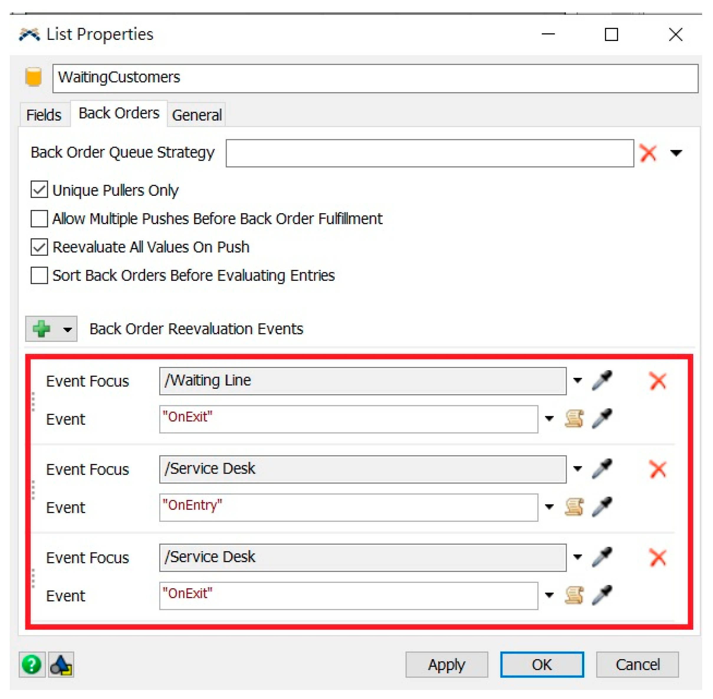
2.1. Resources

The concept of resources was introduced by Genrich Altshuller in 1985, in the form of ‘substance-field resources’, which formed a component of his Algorithm for Inventive Problem Solving (ARIZ). The main contribution of Altshuller is that it expands the current means of a subject (or tool) performing a function unto an object. The simple function model between two objects is expanded into a substance-field model between two objects, as shown in Figure 6. Different fields can provide the same function; thus, the substance-field model expands the ability to solve the problem of a function model using different means [10]. Later, this concept was expanded to include other types of resources, such as functions, information, space, time, and change [11]. Zlotin and Zusman [11] also developed evolutionary resources, which help reveal hidden resources, and considered inventive resources including functions, fields, information, ideas, substances, space, time, and trends. The term ‘resources of change’ (or ‘change resources’, but not ‘resources for change’) means the resources produced by a change to the system. A simple example of a change resource is that a bamboo basket cannot hold water because the basket is not waterproof. However, the addition of a plastic bag set into the basket can make the basket hold water. The resource of the bamboo basket is changed by combing a plastic bag with the basket, such that the poor waterproof feature of the basket is amended, enabling it to hold the water.

The substance-field model can be further expanded to the tool–object–product (TOP) model [12]. This is a graphical model of the problem, shown as a combination of the action tool, action object, and action product in the form of a transformed action object. The TOP model is just an extension of the substance-field model, including the results of useful and harmful interactions. This model makes it possible to compare and identify opportunities for further development and aggregation and has proved its practicality for efficiently forecasting biomedical engineering systems such as Automated External Defibrillators (AED).

Bogatyrev and Bogatyreva [13] proposed the seven stepping-stones algorithm to break down the inventive challenge in a step-by-step way. In the fourth stage, resources are used to create the conditions for the ideal final result. One systematically considers subtle changes to the parameters of all available resources within the system at hand, including the free environmental ones. By applying a nine-window analysis of time and space to the system, one can obtain a full view of the context of the system behaviour and avoid missing any opportunity to employ the existing resources. It is worth noting that Bogatyrev and Bogatyreva [13] worked with Bio-TRIZ, and most of their examples were inspired by biological evolution [14,15]. Bio-TRIZ relies more on information resources than substance resources, which are more environmentally conservative.

Mann [16,17] proposed two ways of identifying the resources within a system. The first is linked to the trend of evolution: from an evolutionary potential radar plot, one can perceive how much further a given system is able to evolve. In these plots, every bit of unused evolutionary potential represents a resource. The second approach is to provide a trigger list of resources that other problem solvers in other fields have at some time, which are successfully harnessed as resources. An example that illustrates the concept of an unused property in an object is shaving cream, which is usually opaque, making it difficult for the user to see where to shave under the cream. A transparent shaving cream was thus produced by Gillette to solve this problem, allowing users to easily notice where to shave. Here, opaqueness was a resource before transparent shaving cream was invented because its property was not being fully utilised.

A resource can be regarded as a function carrier and can be used to perform a function on a receiving object. With proper trimming rules, this resource can be identified. Weaver [18] proposed six trimming rules that are very helpful for function analysis. Using the six trimming rules, one can identify a hidden object in the function analysis and its hidden function, so that the function of another existing component can be trimmed or replaced by the hidden component in the system or supersystem. Sheu and Hou [19] further expanded the six trimming rules and developed a two-loop, depth-first, recursive trimming process to maximise the trimming effect. An industrial case of a slit-valve failure problem was tackled with the algorithm and breakthrough results were presented.

There is a good reference [20] for classifying resources in TRIZ. Since businesspeople have their own concepts about what constitutes a resource, Mueller also extended this to the management field to allow businesspeople to convert their resource concept into TRIZ terms to help solve their management problems. This merging of the understanding of a resource between business and TRIZ has dramatically enhanced the practicality of resources in TRIZ.

Sheu et al. [21] extended the use of resources from “Useless to Useful” and “Harmful to Helpful”. Most people do not consider harmful things to be “resources”. They usually want to avoid or eliminate them rather than taking advantage of them. Breaking such psychological inertia, TRIZ resources proposed the concepts of Useless to Useful and Harmful to Helpful. One intriguing example of exhaust gas emitted from a thermal power plant polluting the environment was used to show its practicality.

For those new to the TRIZ field who want to know the basics of TRIZ philosophies, an excellent reference is the work by Sheu et al. [22]. There, resources are considered one of the seven pillars of TRIZ. Furthermore, the zero-waste concept in lean thinking is compared with the TRIZ resources concept. Zero waste means utilising resources fully within or around the operational system. The abovementioned Useless to Useful and Harmful to Helpful concepts can further complement the zero-waste concept in lean thinking.

None of the above researchers discussed the side effects of using a free resource, especially in the field of software and simulation modelling. Since information and knowledge are two of the key competitive weapons of our time, the companies that have the best information, or wield it most effectively, will win in the competitive market [23,24]. One feels that it is important to discuss the cost of misusing misleading information due to the use of a free resource to trigger the waiting time measurements in a queue.

2.2. Simulation Modelling

One starts with an introduction to the importance of simulation modelling. One reason for this is that the ordinary equations used in queuing theory cannot handle the complexity of a modern logistical system. In order to gain insights into the dynamic behaviour of a complex system, one needs to use simulation modelling [25]. Examples include the flow of people in a railway station [26], ladles travelling through a steel plant [27], or a car frame going through the interior assembly line section in an automobile production plant [28].

Queueing is a common frustration in daily life. When the resources are not sufficient to meet the demand, a queue develops. The problem with queueing is that, in a complex model, it is intractable, making it difficult to find relevant performance indices such as the average content in the queue, the average waiting time in the queue, and the busy status of the server. Thus, a discrete simulation model is used to resolve this problem. Furthermore, a proper queueing strategy was found to help to reduce the queue length and waiting time in a truck assignment task at marine container terminals [29].

The waiting time of a flow item (such as a customer or part) in a system is one of the seven sources of waste in lean production [30]. To reduce the waiting time, one first needs to measure the waiting time that occurs when the flow item remains static and no value-added operations are applied.

One way to address this is the modelling methods used in FlexSim. Suppose that one is interested in knowing the average waiting time in a simple queue with one processor, similar to an M/M/1 system. To make the system more realistic, one adds a limit to the waiting time that the customer will tolerate: if the customer waits more than 200 s, they will become frustrated and leave the system. This system is shown in Figure 1. There is an important issue related to measuring the waiting time, as the 3D model uses an incoming customer to activate the updating of the waiting time of the remaining customers in the queue. Although the use of this measure is very smart, because it avoids the need to apply an additional timer, it means that there will be a measurement error in the waiting time of frustrated customers who leave the system without being served. It is well-known from Maister [31] that an additional waiting time causes customer resentment. Knowing the accurate waiting time of a frustrated customer is very important from a managerial perspective; misleading information regarding waiting times can cause great problems in terms of retaining potential customers.

2.3. Technical Contradiction

Now, one can set a technical contradiction in our 3D model and use the customer joining the waiting line as an event to update the waiting time of the customers in the waiting line. This saves the need for a timer in the simulation model; however, it causes inaccurate measurements of the waiting time of the customers in line. Thus, one can say that the thing they want to improve is ‘resource reduction’, and the thing they worsen is the ‘inaccurate measurement of waiting time’. Put into TRIZ terms, they want to improve feature 26, the amount of substance yet worsen feature 28, accuracy of measurement. The inventive principles (IP) suggested in the contradiction matrix are IP 13, 2, and 28. One can use these IPs to trigger the possible solutions.

IP 13, ‘The other way around’, has three sub-categories:

• Invert the action used to solve the problem (i.e., cooling instead of heating).
• Make a moveable part fixed and a fixed part moveable.
• Turn the object (or process) upside down.

IP 13a implies that instead of using the incoming event of customers in the waiting line, one uses the outgoing event of customers in the waiting line to update the time.

IP 2, ‘Taking out’, has two sub-categories:

• Extract the disturbing part or property from an object.
• Extract only the necessary part of an object.

IP 2b implies using all events to update time (e.g., an incoming customer to the waiting line, outgoing customer from the waiting line, incoming customer to the service desk, and outgoing customer from the service desk.)

IP 28, ‘Replacing the mechanical system’, has four sub-categories:

• Replace a mechanical system with a sensory one (optical, acoustical, thermal, etc.)
• Use an electric, electromagnetic field to interact with an object.
• Replace a stationary field with a moving field, an unstructured field with a structured one.
• Use fields in conjunction with ferromagnetic particles.

IP 28c implies using an additional event from outside to update time. One may set a limit for the measurement error; for example, 30 s. When there is no update in the waiting time for more than 30 s, the system will automatically update the waiting time.

To summarise, the technical contradiction model provides some ideas regarding the solution to our model.

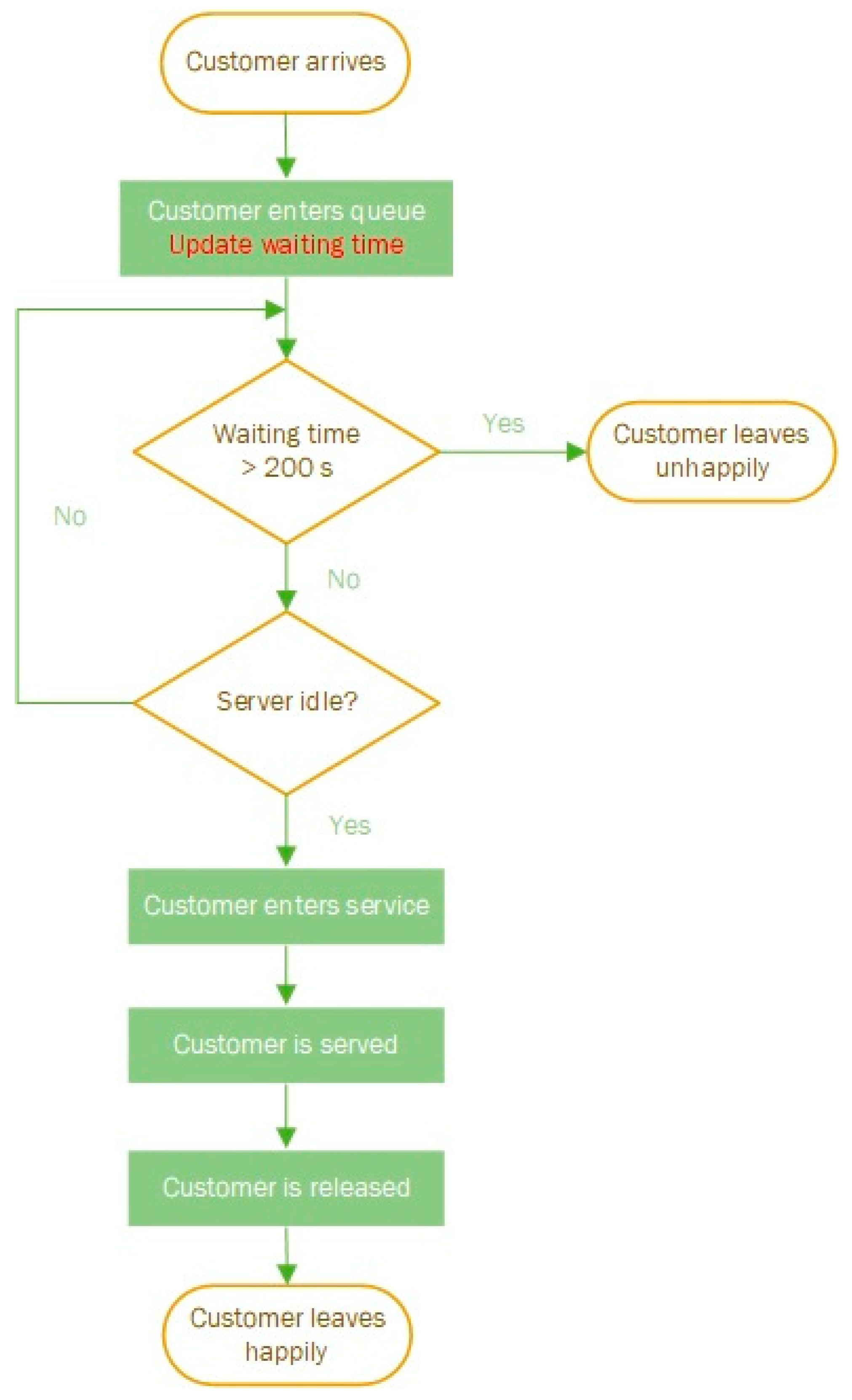
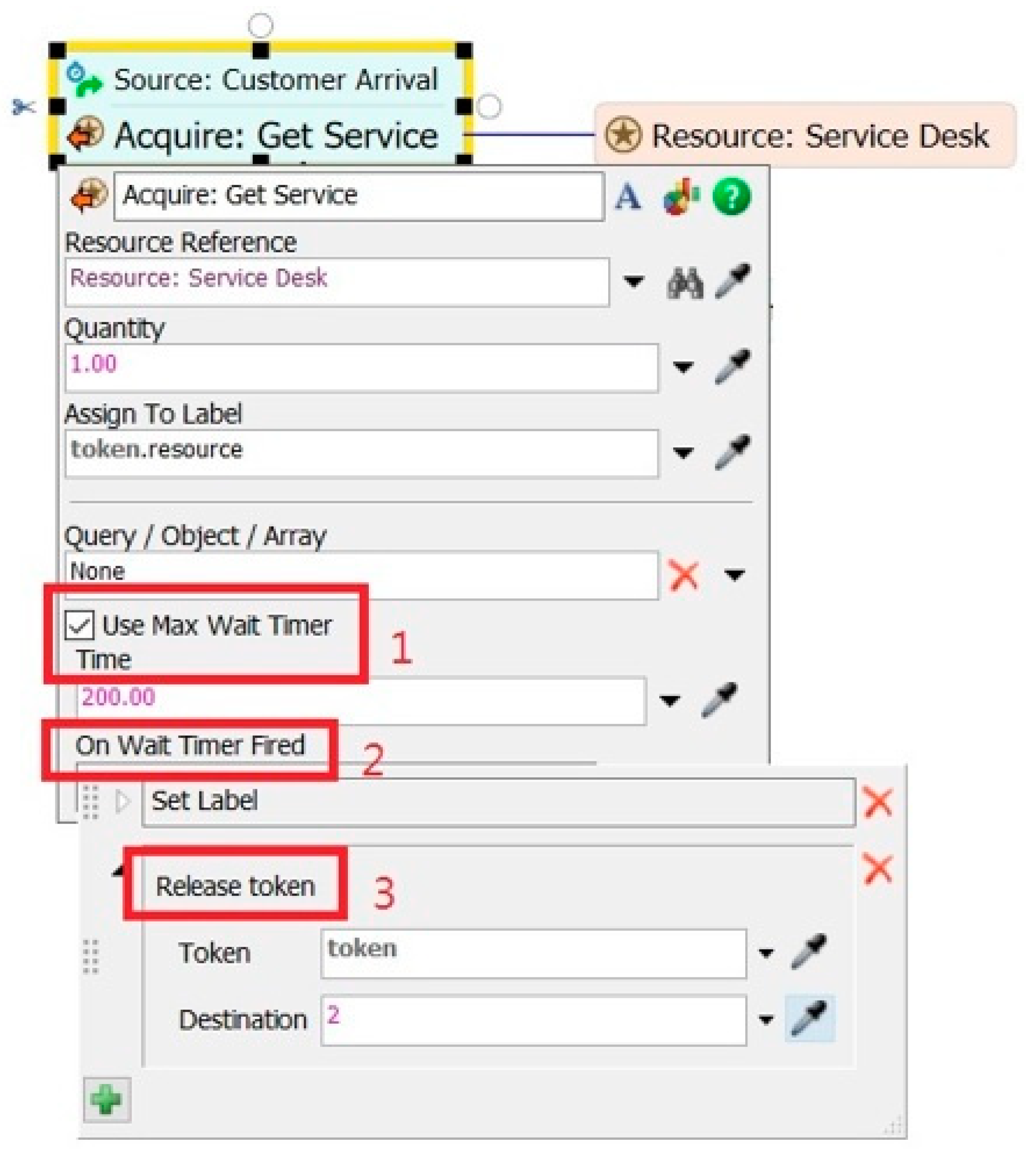
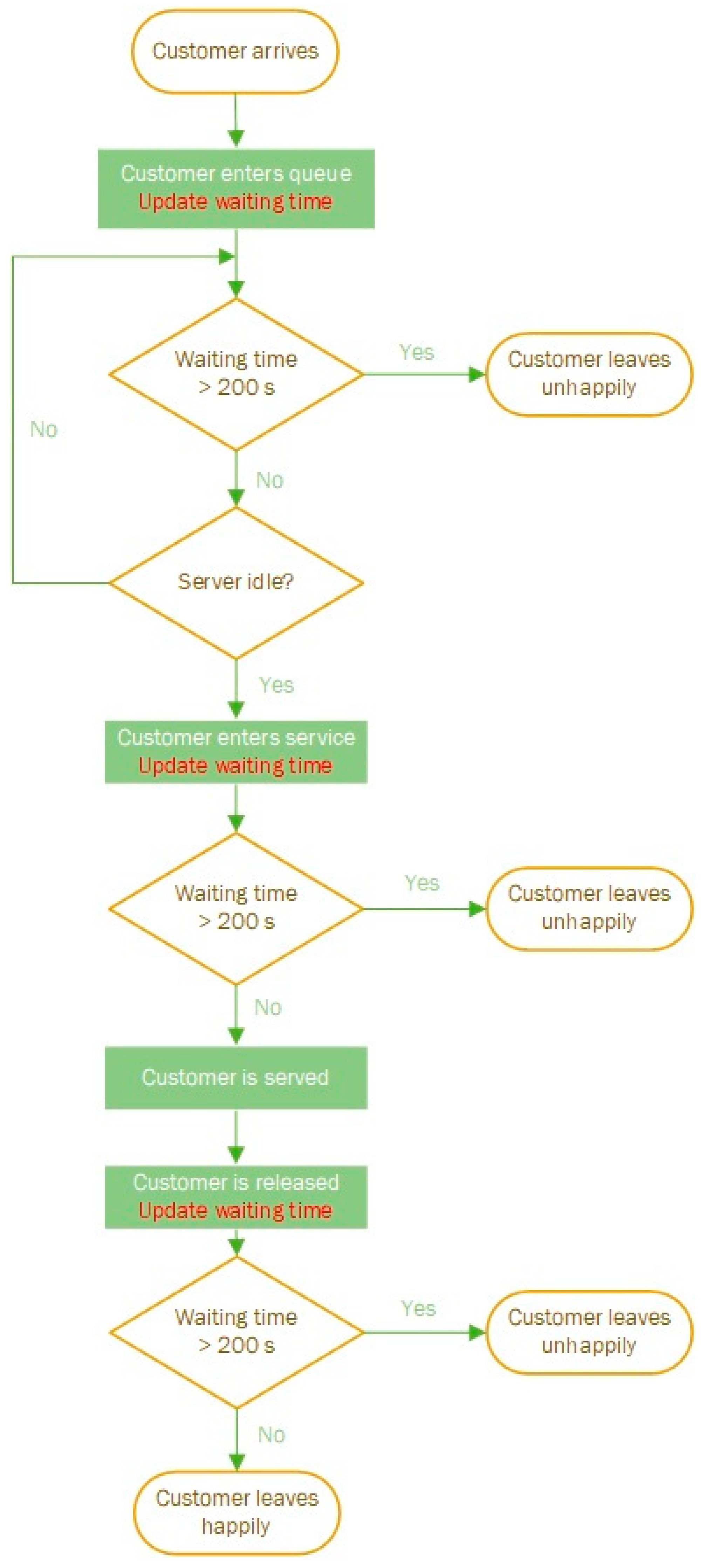
• Use incoming customers to the waiting line to update the time (original alternative provided by the tutorial.) This method is intuitive.
• Use outgoing customers from the waiting line to update the time (this was not thought of in the tutorial.)
• Use incoming customers to the service desk to update the time (this is thinking outside the box.)
• Use outgoing customers from the service desk to update the time (this is thinking outside the box.)
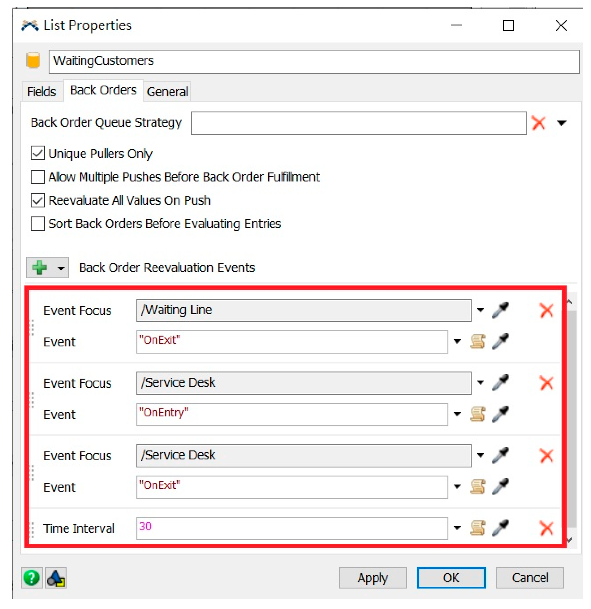
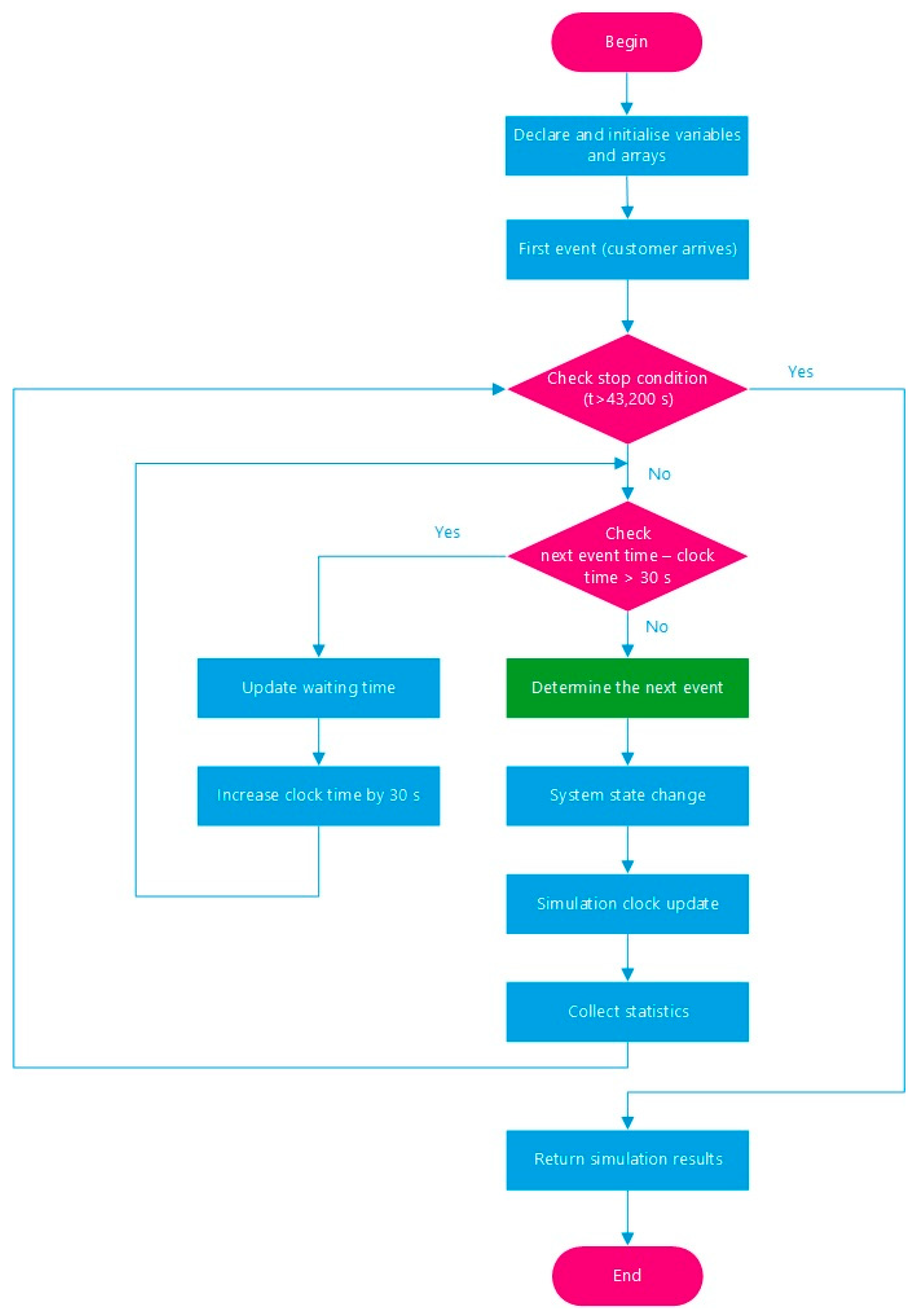
• Use a measurement error limit of 30 s for waiting time and update the waiting time automatically whenever there is no update for more than 30 s (this is thinking outside the box).

In sum, a proper queueing strategy can reduce waiting time. Furthermore, making proper use of a resource to trigger the waiting time calculation can reduce the need to measure the waiting time. The waiting time must be recorded correctly to measure the queueing strategy. The research problem is finding the right TRIZ resources in the discrete simulation modelling to help record the waiting time so that the measurement error can be mitigated without the use of a timer for each customer. This problem is significant because it will provide management with a proper perspective of the queueing system and help them to take prompt action. Without a correct measurement of the waiting time, management could easily be misled, with disastrous effects on the system.

In the following section, one can present a process flow model that provides a counterpart to the 3D model. This model provides a timer for each customer in the waiting line. Then, one can run the 3D model in the tutorial, a histogram of the waiting times in both systems will be compared to show the superiority of the new process flow model. After that, the triggered solution is implemented in the 3D model. Statistical tables of the waiting times will show the improvements in the triggered model.

3. Process Flow Model, 3D Model and Experimental Results

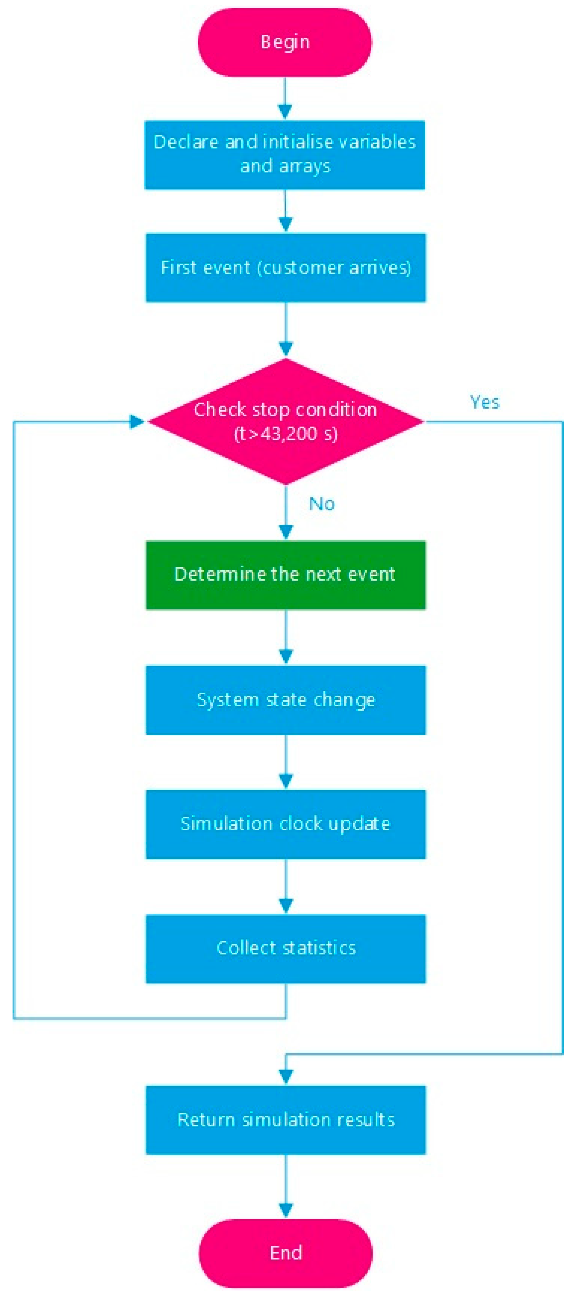
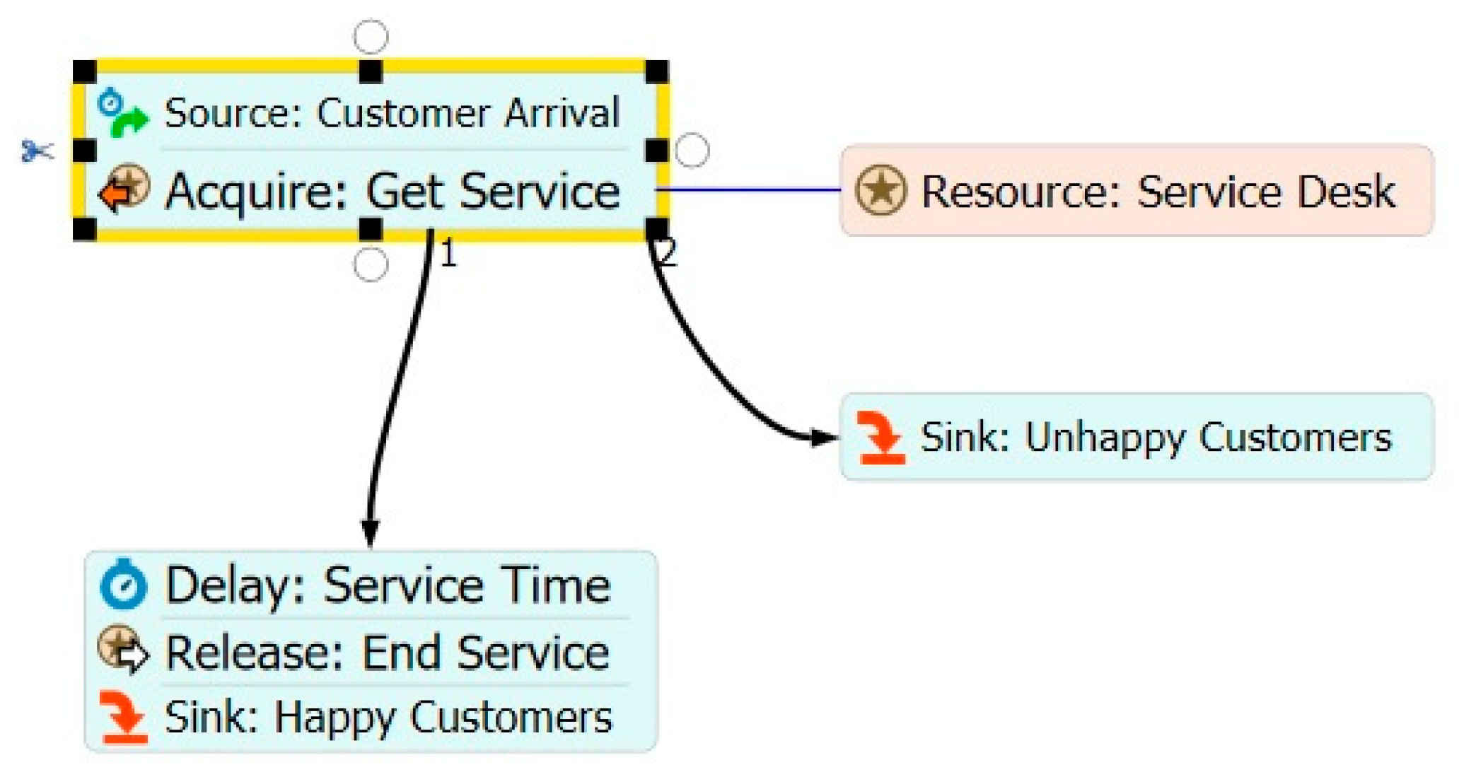
3.1. Process Flow Model

Unlike an object-based 3D model, a process flow uses event activity to represent a modelling system. An activity is similar to a chunk of logic or a logical operation in a simulation model. One advantage of using a process flow tool is the relative ease of creating a logical custom model in this tool. The layout of the process flow corresponding to the 3D model is given below [32]. It should be noted that this process flow model is also taken from a FlexSim tutorial [32]. Figure 7 shows that when a token is created in the inter-arrival source, it will try to obtain a resource before it proceeds to performing the processing work in the service desk. For this reason, the Acquire: Get Service activity is connected to the Resource: Service Desk activity in blue line. There are two connectors from the Acquire: Get Service activity: one is connector 1 to the Delay: Service Time activity and the other is connector 2 to Sink: Unhappy Customers. By default, the Acquire: Get Service activity will connect via connector 1 to the Delay: Service Time activity, meaning that, after acquiring the resource, the token will immediately enter the service desk and receive the service typified by the Delay: Service Time. However, for those waiting in the Acquire: Get Service activity, if their waiting time is more than 200 s, they will be sent to Sink: Unhappy Customers via connector 2, as shown in Figure 8. In this way, the process flow fulfils the requirements for system modelling. One can set up the inter-arrival source with an exponential distribution with a mean of 60 s and the Delay: Service Time with a log normal 2 distribution with a location, scale, and shape of 90, 3.1, and 0.5, respectively. The program ran for 12 h and results were obtained for the process flow, as well as a histogram of the waiting time, as shown in Figure 9 and Figure 10.

From the dashboard in Figure 10, the numbers of unhappy and happy customers are shown to be 302 and 453, respectively. The 302 unhappy customers all waited in the queue for 200 s and constitute the majority of the last bin of the histogram to the right of Figure 9. The values for the minimum, maximum, average, and standard deviation in the waiting time for both unhappy and happy customers are 0, 200, 156.37 and 54.69 s, respectively. If one only considers the waiting times of the 453 happy customers, the values of the minimum, maximum, average, and standard deviation of the waiting times are 0, 199.99, 127.36, and 53.59 s, respectively.

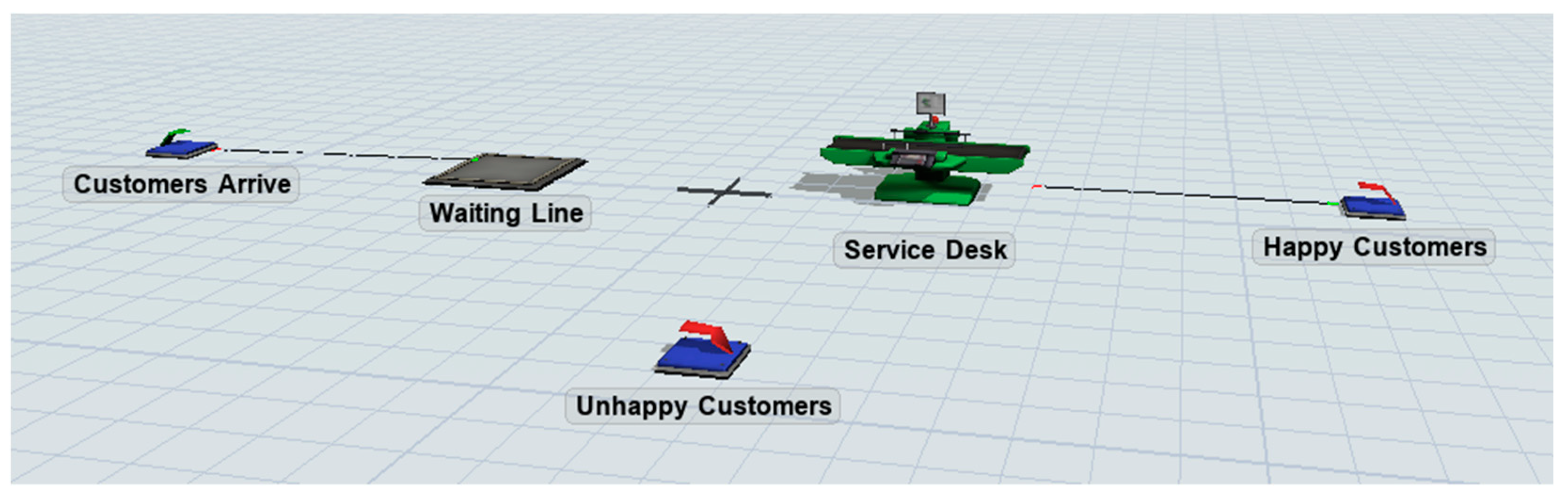
3.2. 3D Model: Default

The 3D model was used to create a histogram of the waiting times for the default case, where only incoming customers are used as a trigger to update the waiting times, and the results are shown in Figure 11. There were 278 and 455 unhappy and happy customers, respectively. Note that these numbers are different from their counterparts (302 and 453) in the process flow, as different random seeds were used, even though the distributions were the same. If one separates the data in Figure 11 into two groups representing unhappy and happy customers, one can obtain the two separate histograms in Figure 12 and Figure 13. Figure 14 shows that, within these 278 waiting times for unhappy customers, the minimum, maximum, average, and standard deviations in the waiting times are 200.10, 398.83, 237.88, and 35.40 s, respectively. For the 455 waiting times for the happy customers, the minimum, maximum, average, and standard deviations in the waiting times are 0, 354.84, 162.38, and 70.88 s, respectively.

Two points are worth noting here. Firstly, the waiting time for happy customers may be more than 200 s. This may sound strange since, if the waiting time is more than 200 s, the corresponding customers should go to the unhappy customers sink; however, the simulation model is based on discrete events. When a customer has waited more than 200 s, they will not be pulled into the unhappy customers sink unless a new customer has entered the queue, which triggers the pulling action from the unhappy customers sink. If, during this time, the service desk becomes available, it will pull the customer with the longest wait, which may be more than 200 s, into the service desk. Thus, it is possible that the waiting time of a happy customer could be more than 200 s. In the records of time spent in the waiting line, the waiting time is regarded as being no more than 200 s, since it is not updated. However, the actual waiting time is more than 200s. This waiting time can be calculated as the difference between the time upon entering the service desk and the time upon entering the waiting line. There were 152 happy customers whose waiting time was more than 200 s, representing 152/455 = 33% of the total.

Secondly, the average waiting time of unhappy customers is 237.88 s. In contrast to the results from the process model, in which the waiting time of an unhappy customer is always 200 s, the modelling results from the 3D model could mislead us. It should also be noted that the calculation of waiting time for happy customers derived from the time the happy customer enters the service desk, subtracting the time the customer enters the waiting line. Similarly, the calculation of the waiting time for unhappy customers is derived from the time the unhappy customer enters the unhappy customer sink, subtracting the time the customer entered the waiting line.

One can explain the waiting time of unhappy customers as follows. The pulling of customers in the waiting line to the unhappy customer sink happens when a new customer enters the waiting line. By then, some customers have waited more than 200 s. Thus, unhappy customers wait for more than 200 s. In our case, the minimum, maximum, average, and standard deviations of the waiting time are 200.10, 398.83, 237.88, and 35.40 s respectively.

3.3. Perspective of TRIZ

Here, these results are discussed from the perspective of TRIZ. As mentioned previously, the use of hidden resources is a clever way to solve a technical contradiction. In the simulation modelling problem, one needs to use a timer to keep track of the waiting time of each customer in the queue, but using a timer imposes a load on the system and slows down the running speed. Thus, the modeller uses a hidden resource, i.e., the event of an incoming customer into the queue, to update the waiting times. In this way, the need for a timer is avoided and the problem is solved. At this point, one might say an ideal solution has been reached in TRIZ terms; however, the ripple effects of this solution and the correctness of the waiting times must be considered. Managers may want to know the correct values of the waiting times so that they can apply proper measures to improve the quality of the service system, but the use of this method jeopardises the waiting time measurement. A new insight can be obtained: when one solves a TRIZ problem, sometimes one is only solving the problem based on a functional analysis, but a related characteristic may be neglected. In our case, this neglected characteristic is the issue of measurement.

3.4. Improvement of 3D Model: Default

Fortunately, this problem can be alleviated using the previously mentioned contradiction matrix. The improvement can be made in three consecutive stages. First, one more event can be added, outgoing customers from the waiting line, to trigger updates to the waiting time of the customers in the waiting line (this is called 3D Model: Stage 1). Second, in addition to the outgoing customers from the waiting line, two more events are added: incoming customers to the service desk and outgoing customers from the service desk (this is called 3D Model: Stage 2). Third, besides the events in the second stage, one more event is added: when the waiting time is not updated for more than 30 s, the system will update it automatically (this is called 3D Model: Stage 3), as described below.

In the first stage, i.e., 3D Model: Stage 1, only a single event has to be added to the Back Order Reevaluation Event tab, as shown in Figure 15. This gives rise to a small improvement, as shown in Figure 16. A comparison of Figure 14 and Figure 16 shows that the average waiting time for happy customers drops from 162.38 s to 158.32 s, whereas for unhappy customers, it drops from 237.88 s to 222.53 s. The corresponding queueing model for the first stage is shown in Figure 17. The corresponding flow chart of the discrete event simulation model in the 3D Model: Stage 1, is the same as the one shown in Figure 5, where “Determine the next event” is substituted by the flow chart in Figure 17.

In the second stage, i.e., 3D Model: Stage 2, the required modification to the Back Order Reevaluation Event is shown in Figure 18. Part of the dashboard after the simulation has been run is shown in Figure 19. Compared with Stage 1, the waiting time for happy customers has been significantly reduced from 158.32 s to 127.13 s; however, the waiting time for unhappy customers does not change much. Indeed, it slightly increases from 222.53 s to 223.74 s, possibly due to the different randomness sequences between these two stages. The corresponding queueing model for the second stage is shown in Figure 20. Note that, by comparing Figure 17 and Figure 20, the event of leaving the queue is shown to be the same as entering the service. Therefore, in both figures, only the event of a customer entering the service updates the waiting time.

In the third stage, i.e., 3D Model: Stage 3, the required modification to the Back Order Reevaluation Event is shown in Figure 21. Part of the dashboard after the simulation has been run is shown in Figure 22. A comparison of Figure 19 and Figure 22 shows that the waiting time for unhappy customers is significantly reduced from 223.74 s to 210.35 s, while the waiting time for happy customers is unchanged. The maximum waiting time for an unhappy customer is 229.77 s since our maximum measurement error for the waiting time is 30 s. One notes that, in the third stage, the corresponding simulation model is different from the one in Figure 5 in that there is a modification to the discrete event simulation model to reflect the event in which the waiting time is updated every 30 s if no update occurs in the queueing model. The new discrete event simulation model is shown in Figure 23.

A comparison of the statistics for waiting times between the process flow model (shown in the Tutorial and the perfect model), default stage (shown in the Tutorial and usually implemented without TRIZ resource knowledge), Stage 1, Stage 2, and Stage 3 (shown with TRIZ resource knowledge) is shown in

Table 1. Statistics of waiting time (in seconds) for aggregates of happy and unhappy customers.

	Min.	Max.	Average	S.D.	Count
Process Flow Model	0	200.00	156.37	54.69	756
3D Model: default	0	398.83	190.97	70.25	734
3D Model: Stage 1	0	294.16	182.59	64.96	725
3D Model: Stage 2	0	292.19	165.38	66.50	740
3D Model: Stage 3	0	229.77	160.08	61.11	740

,

Table 2. Statistics of waiting time (in seconds) for happy customers.

	Min.	Max.	Average	S.D.	Count
Process Flow Model	0	199.99	127.36	53.60	454
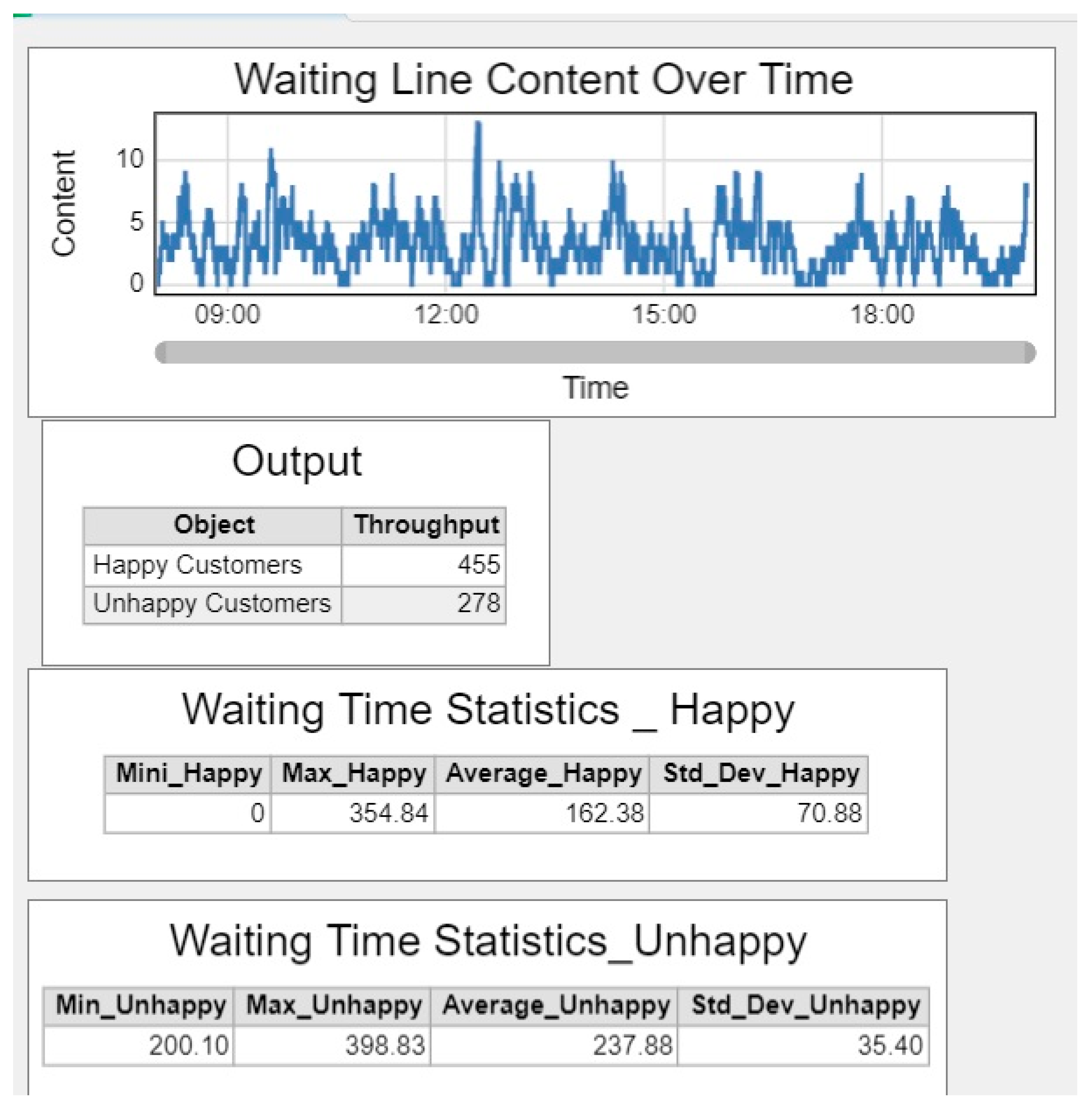
3D Model: default	0	354.84	162.38	70.88	456
3D Model: Stage 1	0	294.16	158.32	70.85	451
3D Model: Stage 2	0	199.83	127.13	58.29	447
3D Model: Stage 3	0	199.83	127.13	58.29	447

and

Table 3. Statistics of waiting time (in seconds) for unhappy customers.

	Min.	Max.	Average	S.D.	Count
Process Flow Model	200.00	200.00	200.00	0	302
3D Model: default	200.10	398.83	237.88	35.40	278
3D Model: Stage 1	200.10	288.15	222.53	18.52	274
3D Model: Stage 2	200.10	292.19	223.74	18.62	293
3D Model: Stage 3	200.10	229.77	210.35	7.96	293

. Table 1 presents the waiting time statistics for aggregates of happy and unhappy customers; Table 2 is for happy customers; Table 3 is for unhappy customers.

It is clear from Table 2 and Table 3 that 3D model: stage 2 can improve the measurement of the waiting time of happy customers, making it the same as the Process Flow Model. Three-dimensional model: stage 3 can even reduce the measurement error in waiting time for unhappy customers within an error of 30 s. In the case of an unhappy customer, by comparing the 3D Model: default to 3D Model: stage 3, the maximum waiting time is reduced from 398.83 s to 229.77 s, the average waiting time from 237.88 s to 210.35 s, and the standard deviation of the waiting time from 35.40 s to 7.96 s. Thus, using the contradiction model to tackle the measurement error problem of simulation in FlexSim triggers ideas that are outside of the box and easily implemented, rendering significant improvements in customer waiting time. Although the application of resources in the simulation is demonstrated using FlexSim, this does not mean that other simulation packages could not be used. The significance of the application of resources with the help of the contradiction matrix and inventive principles in TRIZ is that the proper use of resources can help to reduce the measurement error in the waiting time. These resources may escape the notice of a programmer if the framework of TRIZ is not used.

3.5. Insight of 3D Model: Stage 2

Finally, we will explain why exact waiting times of happy customers are obtained in Stage 2. Recall that, in Stage 2, additional resources were introduced in the form of events in which customers entering and leaving the service desk act as a mechanism to trigger updates to the wait times. The event of a customer entering the service area is the same as the event of a customer leaving the waiting line, since a customer leaving the waiting line must enter the service area to receive service [25].

Although some customers will be pulled into the unhappy exit because the waiting time exceeds 200 s, this mechanism is activated by the unhappy sink, not by the mechanism of customers leaving the waiting line. The results of our simulations confirm this. When an option was added to the Back Order Reevaluation Event to reflect a customer entering the service desk, the statistics for the waiting times of happy customers were the same as those for Stage 1 of the 3D model. Hence, the resource that changes the waiting times of happy customers is the event of leaving the service desk.

As mentioned earlier, in the 3D default model, the waiting time of a happy customer may exceed 200 s. This happens when the customer’s waiting time exceeds 200 s but a new customer has not yet entered the waiting line, as the customer’s waiting time, according to the system records, is still less than 200 s. At this time, if the service area is free, the customer will enter the service area to receive services, meaning that the waiting time of this happy customer will exceed 200 s. This problem of inaccurate measurement can be avoided by making sure that the customer’s wait time is updated when the service area becomes available. This is the aim of Stage 2 of the 3D model. When a customer leaves the service area, the waiting times of the customers in the queue are updated, and the system can determine whether the customer at the front of the waiting line can enter the service area. A customer whose wait time exceeds 200 s is pulled into leaving unhappily, and cannot enter the service area. If the wait time is less than 200 s, however, the customer can enter the service area. In this way, the waiting times of happy customers can be accurately recorded.

Sometimes, when a customer enters the queue, other customers have been waiting for more than 200 s, and the service area is still busy and cannot provide services to these customers. At this time, these customers will be pulled into the unhappy customers’ exit. This creates waiting times of more than 200 s for unhappy customers. To address this problem, a timer must be used. In Stage 3 of the 3D model, if the system has not updated the waiting time within 30 s, it will be automatically updated; however, this approach can only reduce the measurement error to within 30 s.

4. Conclusions

4.1. Summarising the Key Findings

The tutorial example of the queueing model with two possible outlets for customers was used to demonstrate how the TRIZ contradiction matrix can help identify hidden resources in the model and how this resource can mitigate the waiting time measurement errors. Three consecutive resources are highlighted and the average aggregate waiting time error is reduced from 22.13% to 2.37%. The error is reduced from 99.42% to 14.89% for the maximum waiting time. If one considers customer type, the average waiting time error is reduced from 27.50% to 0% for happy customers. The error is reduced from 77.43% to 0% for the maximum waiting time. For unhappy customers, the average waiting time error is reduced from 18.94% to 5.18%. The error is reduced from 99.42% to 13.89% for the maximum waiting time. Thus, these new resources completely solve the measurement error in waiting time in the case of happy customers. For unhappy customers, the error is significantly reduced but not eliminated.

Thus, it is very important for the programmer to use proper resources in simulation modelling. It is recommended that the programmer should learn the basic concept of the contradiction matrix, as illustrated in the paper. This will help him/her to identify the proper resources and improve the quality of their program. Only a few checks in Flexsim are needed to add those resources, so it is worth applying TRIZ resources to their programming practice.

4.2. Concise Recommendation

Resources are very powerful when used to create the conditions for the ideal final result. One important strategy is the use of change resources to adjust the resource parameters so that it fits the conditions for the ideal final result. A change resource is a hidden one, a resource that exists but has not yet been noticed in the context of the problem.

Although many researchers have proposed architectures for implementing resources, none of them focused on the possible side effects of the measurement of a critical value, which, in this case, is the waiting time. It is possible that, without proper consideration of the resource, misleading figures could jeopardise a management decisionThe example of waiting times in a queue in a simple simulation model is used to demonstrate this scenario. This example is taken from a tutorial in FlexSim and sheds some light on the importance of choosing the proper resource to fulfil the system requirements.

4.3. Highlight the Simulation

The simulation of the system starts by generating incoming customers with inter-arrival times that are exponentially distributed with a mean of 60 s. A customer entering the queue waits to be served by the service desk. The service time of the server is a log normal 2 distribution with location, scale, and shape values of 90, 3.1, and 0.5, respectively. There is a second possible destination for the customers in the queue: if they wait for more than 200 s, they will leave the system as a frustrated customer. There are some managerial issues here that need to be addressed. Firstly, the owner of the system needs to know the average waiting times for the two categories (happy and unhappy customers). Theoretically, the waiting time of an unhappy customer is always 200 s; for happy customers, this is always less than 200 s. However, this only holds true if a timer is used for each incoming customer to keep track of the waiting times. Timers take up space in the memory and slow down the running speed of the simulation model; hence, a hidden resource is identified to replace the timer, which is the event of a customer entering the queue. Since the simulation software used is FlexSim, a discrete event-based simulation, the use of a free resource in the form of an incoming customer to trigger updates to the waiting times is very clever, as it reduces the number of objects and simplifies the model. However, it is only effective in terms of function, and one needs to consider the ripple effect on the measurement of the waiting time in the queue.

From a 12 h run of the model, two startling results were found. Firstly, rather than a fixed waiting time of 200 s, the average, standard deviation, and maximum waiting times for unhappy customers were 237.88, 35.40, and 398.83 s, respectively. Secondly, despite the waiting time for happy customers being limited to less than 200 s, there were 152 happy customers whose waiting time was more than 200 s, representing 152/455 = 33% of them. The average, standard deviation, and maximum waiting times for happy customers were 162.38, 70.88, and 354.84 s, respectively.

When one used a process flow to replace the 3D model, the simulation results were similar to the expected results. There were 302 unhappy customers, each of which spent 200 s in the queue. Moreover, there were 453 happy customers, all with waiting times of less than 200 s. The average, standard deviation, and maximum waiting times for happy customers were 127.35, 53.59, and 199.99 s, respectively.

From a comparison of the statistics for the 3D model and the process flow, one can easily see that the results were quite different for both happy and unhappy customers. For unhappy customers, the average waiting time in the 3D model was 237.88 s, whereas for the process flow, this was 200 s. For happy customers, the average waiting time in the 3D model was 162.38 s, whereas for the process flow, it was 127.36 s. The 3D model shows a significant increase (118.9%) in the average waiting time for unhappy customers and this is even larger (127.5%) for happy customers.

Fortunately, these misleading waiting time figures can be alleviated by applying the technical contradiction model to tackle the measurement error problem of simulations in FlexSim. Three resource levels are discovered in the technical contradiction model. Improvements can be made in three consecutive stages. First, one more event can be added: outgoing customers from the waiting line trigger an update to the waiting time of customers in the waiting line (this is called 3D Model: Stage 1). Second, in addition to outgoing customers from the waiting line, two more events are added: incoming customers to the service desk and outgoing customers from the service desk (this is called a 3D Model: Stage 2). Third, besides the events in the second stage, one more event is added: when the waiting time is not updated for more than 30 s, the system will update it automatically (this is called 3D Model: Stage 3).

Using the 3D model: Stage 2, one can completely eliminate the waiting time error in the scenario with a happy customer. Using 3D model: Stage 3, the average waiting time for unhappy customers was 210.35 s, which is about 105.2% of the actual waiting time. Compared with the 3D model: default, the improvement in the average waiting time for unhappy customers in 3D model: Stage 3 was from 118.9% to 105.2%. Note that, for happy customers, this improvement was from 127.5% to 100.0%, which is even greater.

Therefore, through proper consideration of the resources in the simulation modelling in FlexSim, one can significantly improve the measurement of waiting time. Only a few items in the Back Order tab of the global list must be added in order to achieve this. However, without the concepts of resources in TRIZ, simulation programmers could just as easily go with their intuition and miss a major opportunity to improve the quality of the simulation results. Therefore, it is very beneficial to acquire knowledge of the resources in TRIZ, so that hidden resources can be effectively utilised.

4.4. Call to Action

Although the application of resources in the simulation was demonstrated using FlexSim, this does not mean that other simulation packages could not be used. The significance of the application of resources with the help of the contradiction matrix and inventive principles in TRIZ is that the proper use of resources can help to reduce the measurement error in the waiting time. These resources may escape the notice of a programmer if the TRIZ frameowrk is not used.

A final remark may be added for managerial purposes. With business competition becoming more intense due to globalization, resources are a potential sword that can be wielded to solve several associated management problems. It would, therefore, be good practice for managers to acquire some knowledge of these resources and make use of the contradiction matrix to help to identify and manage the resources needed to solve these challenges.

References

- Altshuller, G. Creativity as an Exact Science: The Theory of the Solution of Inventive Problems; Gordon and Breach: New York, NY, USA, 1984. [Google Scholar]
- Deng, J.; Lin, Y.; Tsai, J.; Lee, J. Resolving the OXO measuring cup problem. In Proceedings of the 9th International Conference on Systematic Innovation, Hsinchu, Taiwan, 18–21 July 2018; p. 20. [Google Scholar]
- FlexSim Tutorial: Task 1.1—Build a 3D Model. 2022. Available online: https://docs.FlexSim.com/en/21.0/Tutorials/FlexSimBasics/1-1Build3DModel/1-1Build3DModel.html (accessed on 1 January 2023).
- Jacobs, P.H.M.; Verbraeck, A. Mastering D-SOL: A Java Based Suite for Simulation; Delft University of Technology, Faculty of Technology, Policy and Management, Systems Engineering Group: Delft, The Netherlands, 2006. [Google Scholar]
- Rykov, V.V.; Kozyrev, D.V. On sensitivity of steady-state probabilities of a cold redundant system to the shapes of life and repair time distributions of its elements. Springer Proc. Math. Stat. 2018, 231, 391–402. [Google Scholar]
- Jiamsanguanwong, A.; Ophaswongse, C.; Chansirinthorn, C.; Kitirattragarn, N.; Kittithreerapronchai, O. Improving patients’ experience concerning insufficient informational flow to patients during COVID-19 pandemic: Case study of a traditional Chinese medicine clinic. Int. J. Healthc. Manag. 2023, 16, 51–60. [Google Scholar] [CrossRef]
- Chang, T.Y.; Horng, S.C. Conceptualizing and measuring experience quality: The customer’s perspective. Serv. Ind. J. 2010, 30, 2401–2419. [Google Scholar] [CrossRef]
- Bin Muhmad Pirus, M.S.; Anis, A. Delays of COVID-19 Swab Tests and COVID-19 Laboratory Reports by Private Healthcare Institutions in Shah Alam, Selangor, Malaysia. Glob. Bus. Manag. Res. 2022, 14, 216–225. [Google Scholar]
- Altshuller, G.; Shulyak, L.; Fedoseev, U. 40 Principles, 2nd ed.; Technical Innovation Center: Worcester, MA, USA, 2001. [Google Scholar]
- Belski, I. Improve Your Thinking: Substance-Field Analysis; TRIZ4U: Melboyrne, Australia, 2007. [Google Scholar]
- Zlotin, B.; Zusman, A. The Concept of Resources in TRIZ: Past, Present and Future; Ideation International: Farmington Hills, MI, USA, 2005. [Google Scholar]
- Kernytskyy, I.; Hlinenko, L.; Yakovenko, Y.; Horbay, O.; Koda, E.; Rusakov, K.; Yankiv, V.; Humenuyk, R.; Polyansky, P.; Berezovetskyi, S.; et al. Problem-Oriented Modelling for Biomedical Engineering Systems. Appl. Sci. 2022, 12, 7466. [Google Scholar] [CrossRef]
- Bogatyrev, N.; Bogatyreva, O. Inventor’s Manual; Salisbury Printing Ltd.: Salisbury, UK, 2011. [Google Scholar]
- Vincent, J.F.V.; Bogatyreva, O.A.; Bogatyrev, N.R.; Bowyer, A.; Pahl, A.-K. Biomimetics: Its practice and theory. J. R. Soc. Interface 2006, 3, 471–482. [Google Scholar] [CrossRef] [PubMed]
- Bogatyreva, O.A.; Shillerov, A.E. Biomimetic Management: Building a Bridge Between People and Nature; BioTRIZ Ltd.: Trowbridge, UK, 2015. [Google Scholar]
- Mann, D.L. Hands-On Systematic Innovation, 2nd ed.; IFR Press: London, UK, 2007. [Google Scholar]
- Mann, D.L. Hands-On Systematic Innovation for Business and Management, 2nd ed.; IFR Press: London, UK, 2007. [Google Scholar]
- Weaver, J.B. Systematic Tools for Innovation: The Trimming Technique; Technical Report; University of Detroit Mercy: Detroit, MI, USA, 2009. [Google Scholar]
- Sheu, D.D.; Hou, C.T. TRIZ-based systematic device trimming: Theory and application. Procedia Eng. 2015, 131, 237–258. [Google Scholar] [CrossRef]
- Mueller, S. The TRIZ resource analysis tool for solving management tasks: Previous classifications and their modification. Creat. Innov. Manag. 2005, 14, 43–58. [Google Scholar] [CrossRef]
- Sheu, D.D.; Yen, M.Z. Systematic analysis and usage of harmful resources. Comput. Ind. Eng. 2020, 145, 106459. [Google Scholar] [CrossRef]
- Sheu, D.D.; Chiu, M.C.; Cayard, D. The 7 pillars of TRIZ philosophies. Comput. Ind. Eng. 2020, 146, 106572. [Google Scholar] [CrossRef]
- Stewart, T.A. Intellectual Capital; Doubleday Business: New York, NY, USA, 1997. [Google Scholar]
- Schumacher, E.F. Small Is Beautiful: A Study of Economics as if People Mattered; Hartley & Marks Publishers: Vancouver, BC, Canada, 1999. [Google Scholar]
- Beaverstock, M.; Greenwood, A.; Nordgren, W. Applied Simulation: Modelling and Analysis Using FlexSim, 5th ed.; FlexSim Software Products, Inc.: Orem, UT, USA, 2017. [Google Scholar]
- Kuzmin, D.; Baginova, V.; Ageikin, A. Discrete event simulation model of the railway station. Transp. Res. Procedia 2022, 63, 929–937. [Google Scholar] [CrossRef]
- Wu, S.; Xu, A.; Song, W.; Li, X. Structural optimization of the production process in steel plant based on FlexSim simulation. Steel Res. Int. 2019, 90, 1900201. [Google Scholar] [CrossRef]
- Wang, Y.R.; Chen, A.N. Production logistics simulation and optimization of industrial enterprise based on FlexSim. Int. J. Simul. Model. 2016, 15, 732–741. [Google Scholar] [CrossRef]
- Wang, J.; Huynh, N.N.; Pena, E. Land side truck traffic modelling at container terminals by a stationary two-class queuing strategy with switching. J. Int. Logist. Trade 2022, 20, 118–134. [Google Scholar] [CrossRef]
- Ohno, T. Toyota Production System: Beyond Large-Scale Production; Productivity Press: New York, NY, USA, 1988. [Google Scholar]
- Maister, D.H. The Psychology of Waiting Lines; Harvard Business School: Boston, MA, USA, 1984; pp. 71–78. [Google Scholar]
- FlexSim Tutorial: Task 1.3—Build a Process Flow Model. 2022. Available online: https://docs.FlexSim.com/en/20.0/Tutorials/FlexSimBasics/1-3BuildProcessFlow/1-3BuildProcessFlow.html (accessed on 1 January 2023).