1. Introduction
In recent years, with the rapid development of unmanned autonomous systems, the application fields of unmanned vehicles have become increasingly extensive. After major natural disasters, buildings such as houses and bridges may collapse, forming a sheltered space. Due to the complex environment and narrow and dim space, satellite signals are easily interfered with or blocked, which often leads to the failure of the navigation and positioning of unmanned vehicles in the sheltered space. Therefore, providing accurate, reliable, and real-time navigation information such as position, velocity, and attitude for unmanned vehicles in obstructed spaces is an important guarantee for obtaining disaster information and improving search and rescue efficiency and has significant importance.
Inertial navigation systems (INSs) [
1] have the advantages of small size, easy integration, and pure autonomy, and they are widely used in various navigation fields. However, the errors [
2,
3] of INSs accumulate rapidly over time. INS/GNSS [
4,
5,
6] can obtain higher-precision carrier velocity and position information using the global navigation satellite system [
7] (GNSS). Visual navigation systems [
8,
9] (VNSs) can obtain the high-precision attitude information of a carrier, but they suffer from the drawbacks of increased measurement error in environments with insufficient feature points or significant changes in illumination. Therefore, combining INS, GNSS, and VNS can compensate for their respective shortcomings and further improve the positioning accuracy [
10] of unmanned vehicle navigation systems in complex scenarios.
A centralized Kalman filter [
11,
12,
13] can achieve multi-source fusion navigation using the effective information from various sensors for optimal estimation, thus achieving a higher positioning accuracy. However, as the dimension of the state vector increases, the consumption of computational resources increases, and real-time performance deteriorates. Carlson et al. [
14,
15] proposed a federated Kalman filter [
16,
17] (FKF), which utilizes the principle of information distribution, not only reducing the computational load but also improving the fault-tolerant performance of integrated navigation. In an FKF, all sub-filters evenly distribute the information sharing factor (ISF) [
11,
18,
19] for information sharing. However, in practical applications, the performance and estimation accuracy of subsystems constantly change with the complexity of the navigation environment, and the fixed ISF in an FKF cannot meet the different navigation requirements of the navigation system in complex scenarios.
Lu et al. [
20] combined an odometer with an INS/GPS integrated navigation system and proposed a strategy of using an adaptive information allocation factor, which improved the disturbance rejection capability of the integrated navigation system. Xu et al. [
21] used a dual-state chi-square detection algorithm to calculate the parameters corresponding to each state, ensuring that states with a higher accuracy obtain a larger information distribution coefficient. Zhai et al. [
22] proposed an adjustment strategy using a degree of abnormality to correct the error covariance matrix and Kalman gain, which improved the fault tolerance and accuracy of the positioning system. Shen et al. [
23] proposed a time-varying information sharing factor adaptive federated Kalman filter. In a complex GNSS environment, the proposed adaptive information fusion strategy could autonomously adjust the information sharing factors and their error states of each navigation sensor. Lyu et al. [
24] developed a novel adaptive federated interacting multiple model (IMM) filter for autonomous underwater vehicle integrated navigation systems. The information sharing coefficients of the adaptive federated IMM filter are dynamically adjusted based on the performance of each local system, ensuring the optimal fusion of information from different sources. Xu et al. [
25] developed a robust adaptive federal unscented Kalman filter (RAFUKF) SINS/GNSS/VDM combined navigation algorithm. A federal unscented Kalman filter (FUKF) framework was developed to combine the filter variance with the f-parameter to construct a new ISF and to establish quantitative estimation fault detection mechanisms. Dai et al. [
26] proposed a robust adaptive localization algorithm that utilizes a robust equivalent weight estimation sub-filter and adaptively allocates the information sharing coefficient using the sub-filter state covariance. Jiang et al. [
18] proposed a GPS-AOA-SINS integrated positioning scheme with fault detection inserted between the sub-filter and the main filter. The gain matrix of the fault sub-filter is adjusted in real-time to reduce its impact on the entire system. Chen et al. [
27] improved the filtering accuracy and system stability by constructing a confidence test model to effectively filter out faulty measurement information and adjusting the system noise covariance in real time. Xiong et al. [
28] constructed a simplified state chi-square test(SSCST) for fault detection by using the residuals between actual and predicted observations, and they incorporated a time-varying decay factor into the sub-filters to enhance the stability of the system.
However, most of these studies focused on specific scenarios and single-sensor anomalies, and they lack a discussion on complex and dynamic scenarios [
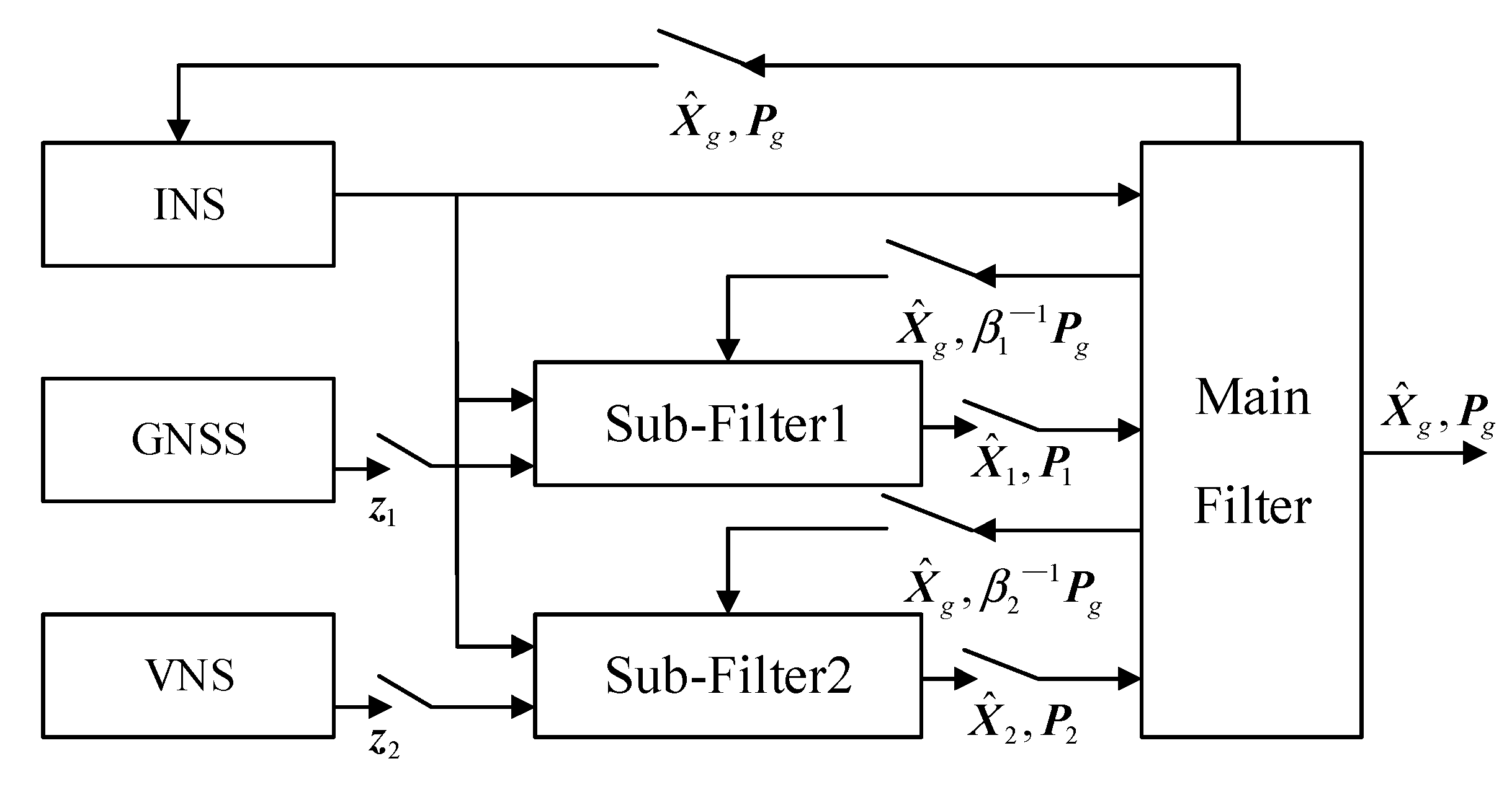
16], as well as different types of sensor failures. In this paper, an improved adaptive federated filter (IAFKF) algorithm based on a federated Kalman filter was designed for the combination navigation system of INS/GNSS/VNS, which is used for unmanned vehicles in obstructed spaces. INS/GNSS and INS/VNS fusion navigation models are established. In the event of possible GNSS and VNS failures, a fault detection algorithm combining the residual chi-square and sliding-window average methods is proposed, which can better detect and isolate fault signals. An adaptive information sharing factor is also proposed to improve the positioning accuracy and fault tolerance by adjusting the error covariance matrix. Finally, the effectiveness of the proposed improved AFKF algorithm was verified through simulation experiments.
The structure of this paper is as follows: In
Section 2, a multi-source fusion model based on federated Kalman filtering is established by combining INS/GNSS and INS/VNS fusion navigation models. In
Section 3, a fault detection method combining the residual chi-square test and sliding-window averaging and an adaptive information sharing factor are proposed. In
Section 4, the effectiveness and real-time performance of the proposed integrated navigation algorithm are verified through simulation experiments. Finally, conclusions are drawn in
Section 5.
3. Improved Adaptive Federated Kalman Filter (IAFKF)
In obstructed spaces, GNSS is prone to positioning anomalies or even satellite unavailability, resulting in a decrease in the positioning accuracy of the integrated navigation system. Additionally, visual navigation systems have poor performance in cloudy or dark environments. Furthermore, since the estimated state values of the federated Kalman sub-filters are fed back to each sub-filter after global fusion by the main filter, the other sub-filters are further contaminated, resulting in positioning errors or even divergence. Therefore, this paper introduces fault detection between the sub-filters and the main filter to detect and process faults in real-time, improving the overall navigation accuracy and fault tolerance.
3.1. Fault Detection
According to the Kalman filter equation, the recursive value at time
k is derived from the previous time
k − 1:
The measurement residual is as follows [
26]:
In this equation,
represents the measurement residual of the
i-th sub-filter at time
k in distributed filtering. When there is no fault in the system, the residual
follows a Gaussian white noise distribution with a mean of 0, and its covariance matrix is as follows:
A fault detection statistic based on the characteristics of the chi-squared distribution can be constructed as follows:
In this equation, follows a chi-squared distribution with m degrees of freedom (the dimension of the measurement Z). If a fault occurs, the residual will no longer be a zero-mean white noise process, and therefore the following method can be used to detect faults.
The fault detection criteria are as follows:
In this context,
represents the fault detection threshold, and
represents the fault flag at time
k. When
, the measurement system has a fault and requires isolation processing. When
, the measurement system is functioning normally. The value of
can be calculated based on Equation (25) and the degree of freedom
m and confidence level using a chi-squared distribution table:
To eliminate occasional abnormal situations, a sliding-window average can be applied to the residual sequence to obtain the actual residual covariance:
Here,
represents the estimated value of the prediction error covariance matrix within the calculation interval
N. The specific value of
N is determined based on experience and the specific situation and is generally chosen to be between 10 and 12. By comparing the trace of the actual covariance of the residuals and the theoretical covariance, we can assess the degree of deviation between the true value and the theoretical value.
where,
is the degree of deviation between the real value and the theoretical value. When the actual covariance of the residuals is generally consistent with the theoretical covariance,
is generally considered to be an indication of a fault-free measurement system. When the actual covariance of the residuals differs significantly from the theoretical covariance, i.e., when
, it is considered to be an indication of a fault in the measurement system.
In this paper, the above two methods are used for fault detection to avoid false alarms or missed detections, thereby reducing the impact of fault signals on the system. If the measurement system fails, the entire system’s state information will be affected after the fusion of the main filter information. In order to ensure the normal stability of the system and avoid the isolation of sub-filters affecting the overall system, a simple compensation method was chosen. That is, when a fault is detected, the estimate of the main filter is used instead of the estimate of the faulty sub-filter.
3.2. Adaptive Information Sharing Factor
In a classic FKF [
14], the information sharing factor is evenly allocated among all the sub-filters. However, this equal distribution method neglects the unique characteristics of each sub-filter, which can result in errors from some sub-filters impacting the positioning accuracy of the main filter. Improper allocation of the information sharing factor can also decrease the accuracy of the integrated navigation system. Therefore, an adaptive allocation of the information sharing factor based on the characteristics of each sub-filter is crucial for improving their performance. To address this issue, this paper proposes an adaptive information sharing factor that can be dynamically allocated based on the state covariance matrix of each sub-filter, reducing the impact of low-precision sub-filters on the positioning accuracy of the main filter. In practical filtering, the state covariance matrix
reflects the precision of the filter, where a smaller
corresponds to a higher accuracy of the filter.
The relationship between the precision
of the sub-filtering system in this paper and the state covariance
is as follows:
where
represents the filtering accuracy of the
i-th sub-filter at time
k, and
tr represents the trace of the matrix. The adaptive information sharing coefficient can be expressed by the precision of the sub-filtering system
as follows:
where
represents the information sharing factor, and
N represents the number of sub-filters. According to Equation (16), the information fusion state of the main filter is as follows:
3.3. Procedure of Improved AFKF
The procedure is shown below:
Step 1: Set the initial values of the filter, including the initial state value , the system noise covariance , and the measurement noise covariance .
Step 2: Time update: the sub-filter performs a time update as per Equations (10) and (11).
Step 3: Measurement update: the sub-filter performs a measurement update as per Equations (12)–(14).
Step 4: Fault detection: using the residual chi-square and sliding-window averaging method for fault detection, the estimated value of the faulty sub-filter is replaced with the estimated value of the main filter as per Equations (21)–(28).
Step 5: Information fusion is carried out as per Equations (15) and (16).
Step 6: Adaptive information sharing factor is calculated as per Equations (29)–(31).
Step 7: Information sharing process is carried out as per Equations (17)–(20).
Step 8: Steps 2 to 7 are repeated in a loop.
4. Simulation Experiment
To verify the effectiveness, fault tolerance, and real-time performance of the proposed improved AFKF for INS/GNSS/VNS integrated navigation, we conducted simulation experiments and compared them with a classic FKF. In the simulation experiments, we set different index parameters for the accelerometer, gyroscope, GNSS, and VNS, as shown in
Table 1. At the same time, we also considered the complexity of the real environment in unmanned vehicle navigation and reasonably set the failure scenarios for GNSS and VNS. In the different scenarios, we compared and analyzed the performance of the different algorithms, and the simulation trajectories are shown in
Figure 2. The running platform for this simulation experiment was an INTEL(R) Core (YM) I5-12500H CPU with 16.00 GB of memory, and the simulation software used was the PSINS toolbox under matlab2022a, which was developed by Professor Gongmin Yan from Northwestern Polytechnical University, which can be used for simulation experiments of integrated navigation systems.
The initial position (local coordinates) was set to , the initial attitude (pitch, roll, yaw) was set to , and the initial velocity (local coordinates) was set to [0 m/s, 0 m/s, 0 m/s]. This corresponded to a simulation of an unmanned vehicle going downhill, uphill, and around corners in an unmanned vehicle trajectory.
In order to simulate the complex environment that unmanned vehicles may encounter in obstructed spaces, we simulated two scenarios. Scenario 1 involved a situation where only the GNSS signal was interfered with or obscured. Scenario 2 involved a situation where both GNSS and VNS were interfered with.
4.1. Scenario 1
This scenario involved a simulation of the GNSS signal being subjected to different degrees of interference or occlusion during the driving of an unmanned vehicle in obstructed spaces. The two time periods were as follows:
Period 1: a time period between 250 s~400 s, where the GNSS signal was weakly interfered with or blocked, and a 10-fold measurement error was added to the GNSS positioning measurement, as shown in Equation (32):
Period 2: a time period between 600 s~750 s, where the GNSS signal was strongly interfered with or blocked, and a 20-fold measurement error was added to the GNSS positioning measurement, as shown in Equation (33):
Here,
represents the true position information,
represents the attitude error of the visual navigation, and
represents a
matrix of a standard normal distribution. The comparison between the improved AFKF proposed in this paper and a classic FKF is shown below. The results of the INS/GNSS/VNS integrated navigation position and velocity errors are shown in
Figure 3a,b, and the three-axis position and velocity errors are listed in
Table 2.
It can be seen that in periods 1 and 2, when the GNSS was subjected to different degrees of interference or obstruction, the improved AFKF proposed in this paper performed significantly better than the classic FKF. In all periods, compared with the classic FKF, the three-axis position average error of the improved AFKF decreased by 62.8%, 60.4%, 69.1%, and the three-axis velocity average error decreased by 79.7%, 77.9%, and 68.4%, respectively.
4.2. Scenario 2
Simulating the driving process of unmanned vehicles in an obstructed space may result in GNSS signal interference or blockage, as well as a shortage of feature points due to environmental issues in VNS. In this simulation, these situations occurred during different time periods.
Period 1: a time period between 250 s~400 s, where the unmanned vehicle drove into a dark scene where there were fewer feature points, which caused a malfunction in the visual navigation. Therefore, a 10-fold measurement error was introduced in the visual positioning. The following formula (34) shows this, where
is the true position information,
is the visual navigation position error, and
is a
matrix of the standard normal distribution:
Period 2: a time period between 600 s~750 s; considering that an unmanned vehicle may drive into certain areas with strong signal interference or obstructed spaces, which can cause GNSS navigation to fail, a 20-fold measurement error was introduced in the GNSS positioning. The following formula (35) shows this, where
is the true position information,
is the GNSS navigation velocity and position error, and
is a
matrix of the standard normal distribution:
The comparison between the improved AFKF proposed in this paper and a classic FKF is shown below. The position and velocity error results of the INS/GNSS/VNS integrated navigation are shown in
Figure 4a,b, and the average errors of the position and velocity of the combined navigation are listed in
Table 3.
Through the analysis of the results shown in
Figure 4a,b and
Table 3, it was found that when the simulated unmanned vehicle experienced failures in satellite navigation and visual navigation during time periods 1 and 2, the improved AFKF proposed in this paper performed significantly better than the classic FKF. Without interference to the navigation signal, the improved AFKF showed a 35.4% reduction in the position error and a 54.8% reduction in the velocity error compared to the classic FKF. Across all the time periods, the improved AFKF exhibited an average reduction of 25.1% in the position error and 62.4% in the velocity error compared to the classic FKF.
In order to prevent the randomness of non-Gaussian noise and verify the adaptive and fault detection capabilities of the algorithm proposed in this paper, the system was subjected to 50 independent simulations in scenario 2, and the root mean square error (RMSE) of these 50 simulations was calculated as a performance metric. The definition of RMSE is as follows:
where
N represents the experiment time, and
and
represent the true value and estimated value, respectively, of the state at time step
k. The final results are shown in
Figure 5a,b. The average root mean square position error and the average root mean square velocity error of the 50 simulation experiments are listed in
Table 4.
From
Figure 5a,b and
Table 4, it can be seen that in these INS/GNSS/VNS integrated navigation simulation experiments, the position and velocity errors determined using the improved FKF proposed in this paper were significantly smaller than those using the classic FKF. The average root mean square errors of the position in the three directions of east, north, and up decreased by 56.4%, 54.8%, and 43.4%, respectively, and the average root mean square errors of the velocity in the three directions of east, north, and up decreased by 71.0%, 72.1%, and 28.4%, respectively.
In order to validate the real-time performance of the proposed improved AFKF algorithm, using the same simulation software and platform as described above and with the same raw data, we compared the entire filtering process time between the improved AFKF and the classic FKF in 50 simulation experiments, as shown in
Figure 6. The driving time of the unmanned vehicle in the simulation was 887.5 s, with an average runtime of 11.2493 s for the improved AFKF and 10.3526 s for the classic FKF. Although the average runtime of the improved AFKF proposed in this paper was increased by 8.66% compared to the classic FKF, it still met the real-time requirements of the integrated navigation of unmanned vehicles. The filtering cycle of the improved AFKF was 1 s, and the INS update period was 0.02 s. The average filtering time was less than 3.69 ms, which was smaller than the INS update period, satisfying the real-time requirements of the system.
To further verify the effectiveness of the algorithm, we conducted simulation experiments on the Gazebo platform, an open-source robot simulation platform that relies on the popular robot operating system (ROS), as shown in
Figure 7a. The unmanned vehicle model used in the simulation experiment was the TurtleBot3-Waffle-Pi, which is a widely used open-source robot for research and education. It is small in size and highly scalable, and the main model parameters and movements used during the simulation are shown in
Table 5. As shown in
Figure 7b, an environment for the unmanned vehicle to travel in was constructed on the Gazebo platform, and the unmanned vehicle traveled at a constant speed of 0.26 m/s. The improved AFKF algorithm proposed in this paper was used to locate the movement of the unmanned vehicle, and the reference trajectory is shown in
Figure 8.
From
Figure 9, it can be observed that in the simulated environment, the unmanned vehicle’s GNSS measurement errors increased due to occlusion. Compared to the classic FKF algorithm, the improved AFKF algorithm reduced the position error by 35.1% and the velocity error by 61.0%.


