Spatiotemporal Heterogeneous Effects of Built Environment and Taxi Demand on Ride-Hailing Ridership

Abstract

Researchers have applied a series of global models to investigate the link between the built environment and ride-hailing ridership based on ride-hailing data from one specific transportation network company (TNC). However, these research designs inadequately represent real ride-hailing demand within a specific spatial range and cannot reflect spatiotemporal heterogeneity in the link. For the first time, this study collects all demand data of TNCs in Nanjing and analyzes their relationship with the built environment. The effect of taxi demand is considered. We adopt a multiscale geographically weighted regression model to account for the spatial non-stationarity and the multiscale effect of each built environment variable. The findings reveal spatiotemporal heterogeneous relationships of the built environment with ride-hailing ridership. Although the relationship between taxi and ride-hailing ridership varies across spatial locations, ride-hailing always acts as a cooperator for traditional taxis. The findings provide implications for policy making, urban planning, and travel demand management of ride-hailing.

1. Introduction

Ride-hailing connects passengers and drivers through smartphone applications developed by transportation network companies (TNCs) and enables passengers to call and ride vehicles [1,2]. Owing to its advantages, such as flexibility and convenience, the usage of ride-hailing services has substantially grown, which has incubated a large number of TNCs. For instance, as one of the major sharing economy markets, China has a total of 313 TNCs that have obtained licenses for online ride-hailing platforms [3]. Policy makers and transport practitioners expect to fill mobility gaps and improve transport accessibility in areas with lower levels of transit services [4]. In contrast, increasing ride-hailing usage may have some negative impacts, such as traffic congestion and public safety [5].

The debate regarding the mixed effects of ride-hailing increases research interest from scholars and transport practitioners who attempt to promote transport policies and planning strategies to support the sustainable development of transportation. In this regard, it is vital to identify the determinants of ride-hailing ridership and how these factors work [2]. The literature suggests that the decisive factors of ride-hailing ridership vary from socio-economics, multi-modal infrastructure to the built environment [1,6,7,8]. Understanding the link between the built environment and ride-hailing ridership not only assists urban planners and policy makers in developing sustainable built environment planning strategies but also helps TNCs to optimize and manage their ride-hailing services.

Although a variety of studies have attempted to understand the links between the built environment and ride-hailing ridership patterns, several gaps need to be filled in the literature. First, as TNCs are not willing to share their data, most studies commonly use the order data of one specific TNC (e.g., Didi or Uber) to represent ride-hailing demand [1,4,9]. However, data from a single TNC cannot depict a complete picture of urban mobility. In reality, multiple TNCs provide ride-hailing services within the same city; thus, analyses based on the order data of one specific TNC may lead to inappropriate policy implications. Moreover, ride-hailing has been introduced as an essential supplement to the traditional taxi industry; however, it is unclear whether taxi ridership has a competitive or complementary effect on ride-hailing ridership [10]. The debate may come from incomplete demand data in prior studies. Second, a considerable number of methods have been applied to explore the effects of the built environment on ride-hailing ridership [1,9,11]. Owing to the spatial variations of built environment effects, it is necessary to consider spatial non-stationarity to explore the relationship between the built environment and ride-hailing ridership. The geographically weighted regression (GWR) can capture the spatial changes in the built environment and effectively explain the spatial heterogeneity of the impact of built environment characteristics on ride-hailing ridership. Therefore, GWR usually outperforms global regressions [6,11]. However, GWR assumes that built environment effects vary at a single spatial scale based on the same bandwidth; ignoring various built environment characteristics usually produces effects on diverse ranges of neighborhood environments [12].

Aiming to fill the above gaps, this study explores the spatiotemporal relationship between the built environment and ride-hailing ridership, considering the effect of taxi ridership. This study contributes to the literature in two ways: (1) We collect demand data for traditional taxis and ride-hailing of all TNCs in Nanjing. Such data make the paper, to the best of our knowledge, the first attempt to explore the links between the built environment, taxi ridership, and ride-hailing ridership within an entire city. (2) We capture the spatiotemporal variations in the effects of different built environment variables on ride-hailing ridership based on a MGWR, which processes the independent variables in different bandwidths and their spatial variation effects. To characterize spatial contexts and obtain a precise relationship between the built environment and ride-hailing ridership, a multiscale GWR (MGWR) model, which can accommodate the spatial non-stationarity and the multiscale effect of each built environment variable simultaneously, is necessary. The findings provide policy implications for transport practitioners and urban planners on a finer scale.

The rest of the paper is organized as follows. Section 2 reviews related studies on ride-hailing ridership, including data sources and the impact relationship between the built environment and ride-hailing ridership. Section 3 introduces the study area, data, and modeling approach. Section 4 presents and discusses the modeling results. At last, Section 5 concludes the study.

2. Literature Review

2.1. Understanding Ride-Hailing Ridership with Different Data Sources

The literature has attempted to understand ride-hailing ridership patterns and their influencing factors based on various kinds of data [5,13,14], among which questionnaire survey is one of the most common data sources. For instance, Deka and Fei [14] explored the factors of ride-hailing trip frequency based on the National Household Travel Survey. The findings show that younger and well-educated people tend to use ride-hailing services more frequently. Ghaffar et al. [13] found that temperature and the built environment are also determinants of ride-hailing ridership, except for socio-economics, based on survey data from Chicago. Apart from the above analyses based on large-scale survey data, some researchers have explored ride-hailing ridership patterns based on surveys of ride-hailing users [13,15]. Using two separate survey datasets for ride-hailing and taxi users, Rayle et al. [5] demonstrated significant differences in user characteristics and wait time between the two categories of users. Tang et al. [15] surveyed ride-hailing users through the ride-hailing platform and demonstrated the impact of ride-hailing usage on travel behavior. In another example, an online questionnaire survey was conducted for Uber users, and the impact of ride-hailing usage on vehicle kilometers traveled (VKT) was investigated [16]. The results showed that ride-hailing usage caused increases in VKT.

Apart from survey data, emerging big data (e.g., order data) provide a different perspective for understanding ride-hailing ridership patterns. Although it is widely believed that emerging big data contain more activity information, TNCs are not willing to share their data [17]. Aiming to better understand ride-hailing ridership patterns, some companies have released a part of their data in recent years. Based on operation data from Didi, He [17] used multi-day ride-hailing order data to understand spatiotemporal mobility patterns from both the regional and driver’s perspectives. Du et al. [18] analyzed the spatiotemporal variations in ride-hailing demand in Haikou. Using the ride-hailing order data collected in Chengdu, Zhang et al. [19] identified areas with high travel intensity and further explored the relationship between points of interest (POIs) and the number of ride-hailing trip orders. However, most prior studies analyze ride-hailing demand based on order data from one specific TNC, which cannot reflect the real demand for ride-hailing due to the state of multi-company competition. Moreover, the literature usually neglects the role of taxi ridership in affecting ride-hailing ridership.

2.2. Built Environment Effects on Ride-Hailing Ridership

As an emerging transport mode, ride-hailing ridership and its relationship to built environment variables have received increasing research attention [14,18,19]. However, the debate on the link between the built environment and ride-hailing ridership has not reached a consensus. Most prior studies suggest that the built environment plays an essential role in affecting ride-hailing ridership [6,9,11,20]. For instance, Yu and Peng [20] used a structural equation model (SEM) to explore the impacts of built environment variables on ride-hailing ridership and found that population density and land use mix show positive relationships with ride-hailing ridership. Similarly, Sabouri et al. [9] found that activity density and land use mix are positively correlated with ride-hailing ridership based on Uber order data. In contrast, Wang and Noland [1] found a negative correlation between land use mix and ride-hailing ridership.

An essential reason for the dissonance in this theme of studies is that researchers often ignore the spatiotemporal heterogeneity in the link between the built environment and ride-hailing ridership [11]. In the previous literature, ordinary least square (OLS) regression is widely used in various fields of research [21,22]. It is also commonly used as a global model for regression in the study of the impact of the built environment and ride-hailing ridership. They assume that the relationship between ride-hailing ridership and influencing factors is spatially constant, and cannot address spatiotemporal issues [2,7]. To account for the spatial effects, Dean and Kockelman [23] considered the spatial error model and spatial autoregressive model to explore the effects of the built environment on ride-hailing ridership. The results showed that the increase of jobs in the retail and entertainment industries had a positive effect on ride-hailing ridership, while pedestrian infrastructure and areas far away from public transport sites had reduced the ride-hailing service. In another example, Gehrke [4] explored the effects of neighborhood-built environment variables on Uber demand based on hierarchical linear models, identifying socioeconomic and built environment factors most associated with any changes to Uber service area size. As these models assume that the coefficients of the independent variables are constant in space, and only capture part of the spatially varying effects, GWR models are then introduced in exploring the spatially heterogeneous effects of the built environment on ride-hailing ridership [2]. For instance, Zheng et al. [24] used GWR models to explore the relationship between the built environment and ride-hailing ridership. The results confirm that the effects of the built environment vary across spatial locations of the study area. Li et al. [11] found that built environment variables, such as road density and population density, showed spatially heterogeneous effects on ride-hailing ridership based on GWR. The literature suggests that GWR often performs better than global models in studies examining the spatial patterns and determinants of ridership [25]; however, as a local regression model, GWR regards the spatial scale constant across space. Built environment variables may have multiscale spatial effects, and such an assumption may cause biased estimations. In order to overcome this issue, Fotheringham et al. [26] proposed a MGWR model that can relax the limitation of fixed bandwidths and consider spatial heterogeneity and scale effects. Mansour et al. [27] applied the MGWR model to examine the relationship between sociodemographic characteristics and COVID-19 incidence rates. An et al. [12] investigated the association between the built environment and public transportation preferences. The above research verified the superiority of the MGWR model.

Overall, although many studies have investigated the determinants of ride-hailing ridership, most analyses are conducted based on operation data collected from one specific TNC. The single data source limits the possibility of mining the relationship between the built environment and real ride-hailing demand. Meanwhile, the impacts of taxi ridership are rarely considered. More importantly, most studies overlook the fact that different built environment variables usually show effects on various ranges of neighborhood environments, and thus the global models and GWR cannot accommodate spatial non-stationarity and the multiscale effect of each built environment variable simultaneously. This study fills the above gaps by collecting ride-hailing ridership data for all TNCs in Nanjing city and examining the scale effects of the built environment on ride-hailing ridership. Additionally, the impacts of taxi ridership are considered.

3. Methodology

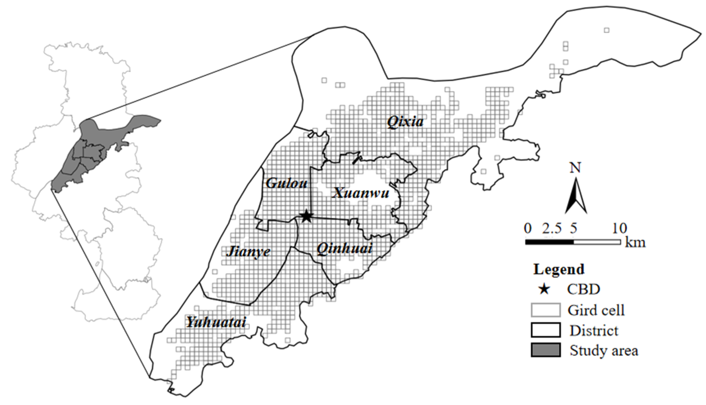
3.1. Study Area and Data

The study area is defined as central Nanjing city, encompassing six administrative districts, namely the Xuanwu, Qinhuai, Jianye, Gulou, Yuhuatai, and Qixia districts. These districts collectively cover an area of 787.45 km². Each district holds unique significance within the city. Xuanwu district serves as a hub for science, education, and tourism. The Qinhuai district stands out as a historical and cultural center. The Jianye district represents a newly developed international region. The Gulou district serves as the economic, cultural, educational, and administrative core. The Yuhuatai district has witnessed significant growth in high-tech industries and serves as a demonstration zone for a renowned software city. The Qixia district acts as a significant shipping logistics center. Hence, this study area effectively captures the essence of urban life in Nanjing. To account for the modifiable areal unit problem (MAUP), we divide the study area into homogenous square grids measuring 500 m × 500 m, rather than relying on traffic analysis zones or administrative units. This grid size aligns with past research conducted on Chinese metropolises [28,29,30]. In total, our analysis utilizes 1555 grids, as depicted in Figure 1.

The endogenous variable is the number of ride-hailing pick-ups in each grid. To better understand the link between built environment variables and ride-hailing ridership, the impacts of the corresponding taxi ridership are considered in this study. The ride-hailing and taxi order data are obtained from the regulatory platform of the Nanjing Transport Bureau. In order to focus on the impact of the built environment on ride-hailing ridership on weekdays, avoid holiday interference, and consider that ride-hailing ridership is cyclical, the data of ride-hailing and taxi orders data from April 11th (Monday) to April 15th (Friday) 2022 are selected for research. In the dataset, each record contains some key information, including order ID, vehicle ID, times, longitudes, and latitudes of pick-ups and pick-offs (

Table 1. Examples of ride-hailing and taxi orders in the dataset.

Order ID	Vehicle ID	Pick-Up Time	Pick-Off Time	Pick-Up Location (Longitude, Latitude)	Pick-Off Location (Longitude, Latitude)
BZ220411011142013000XXX	SAXXX072	2022/04/11 01:15:37	2022/04/11 01:49:57	(118.732278, 32.140057)	(118.895874, 32.053261)
TS120220411013200XXX	SAXXX201	2022/04/11 01:36:01	2022/04/11 01:47:08	(118.842107, 32.122716)	(118.873526, 32.109904)
152faeb379cfe4732XXX	SAXXX1J	2022/04/16 15:51:01	2022/04/16 15:56:02	(118.786830, 32.019600)	(118.787778, 32.012594)
149fd1150121e482eXXX	SAXXX1V	2022/04/11 12:21:27	2022/04/11 12:25:03	(118.774900, 31.967450)	(118.762545, 31.971193)
TS120220416183404XXX	SAXXX282	2022/04/16 18:38:20	2022/04/16 18:45:30	(118.921599, 32.101403)	(118.915473, 32.110716)
TS120220412123602XXX	SAXXX300	2022/04/12 12:40:13	2022/04/12 12:48:15	(118.759594, 32.079994)	(118.772129, 32.069341)

). After removing the records beyond the study area and those with order times less than 2 min or more than 2 h, 835,370 ride-hailing records and 195,691 taxi records are used in this study.

The spatial and temporal distributions of ride-hailing and taxi ridership are visualized in Figure 2. From a spatial standpoint, both ride-hailing and taxi ridership exhibit higher concentrations in urban central areas, gradually decreasing as one moves away from these central regions. Regarding the temporal aspect, ride-hailing and taxi ridership demonstrate similar patterns during workdays. Generally, two peaks can be observed at approximately 8:00 and 18:00, respectively. Consequently, to gain a deeper understanding of the spatiotemporal variations in the relationships, this analysis focuses on two peak periods (7:00–9:00 and 17:00–19:00) as well as an off-peak period (11:00–13:00) on weekdays. As shown in

Table 2. Statistical descriptions of endogenous variables.

Variable	Description	Mean	S.D.
Ride-hailing ridership at morning peak	Number of ride-hailing pick-ups in each grid at weekday morning peak within one week	86.33	110.177
Taxi ridership at morning peak	Number of taxi pick-ups in each grid at weekday morning peak within one week	22.16	34.7
Ride-hailing ridership at off-peak	Number of ride-hailing pick-ups in each grid at weekday off-peak within one week	49.15	73.376
Taxi ridership at off-peak	Number of taxi pick-ups in each grid at weekday off-peak within one week	11.49	35.73
Ride-hailing ridership at evening peak	Number of ride-hailing pick-ups in each grid at weekday evening peak within one week	80.03	114.719
Taxi ridership at evening peak	Number of taxi pick-ups in each grid at weekday evening peak within one week	13.8	33.102

, the total number of ride-hailing and taxi trips is computed for each grid within these three periods over the course of one week.

The built environment variables are selected in terms of the 5D principle [31], including density, diversity, design, distance to transit, and destination accessibility. To capture these variables, a variety of data sources have been utilized. Population density and housing price are employed as measures of the density dimension. Population density is extracted from the University of Southampton (https://www.worldpop.org/ for detail, accessed on 28 June 2023), which provides the population size of global cities based on a 100 × 100 m geographical grid. The housing price is extracted from the Anjuke website (http://anjuke.com/ for details, accessed on 28 June 2023), which is one of the largest online housing brokers in China. The design dimension is measured with road density and bike lane density. Road density and bike lane density are calculated based on the ratios of road lengths and bike lane lengths to the grid area. The road and bike lane lengths are extracted from OpenStreetMap (https://www.openstreetmap.org/ for detail, accessed on 28 June 2023). Destination accessibility is measured with the distance from the centroid of a grid to the Central Business District (CBD). Distance to transit is measured with four variables: bus stop density, metro station density, distance to the nearest bus stop, and distance to the nearest metro station. The bus stop and metro station locations are obtained from AMAP.com, which provides various categories of POIs. In addition to these facilities, thirteen categories of POIs (i.e., restaurants, malls, transport facilities, financial institutions, hotels, educational and cultural facilities, scenic spots, living service facilities, residences, leisure and entertainment facilities, medical facilities, sports facilities, government agencies, and social organizations) are used to obtain the land use mix, which is a common measurement of the diversity dimension. The land use mix is calculated as follows:

$$Entropy=\frac{-{\displaystyle \sum P_i\times \ln P_i}}{\ln n}$$

(1)

where P_i represents the ratio of each category of POIs, and n is the number of categories of POIs.

The statistical descriptions of the built environment variables are shown in

Table 3. Statistical descriptions of the built environment variables.

Variable	Description	Mean	S.D.
Density
Population density	Population size divided by the grid area (thousand persons/km2)	12.641	19.460
Housing price	Average housing prices in the grid (thousand yuan/m2)	16.904	19.683
Diversity
Land use mix	The entropy value of thirteen categories of POIs	0.793	0.208
Design
Road density	Road lengths divided by the grid area (km/km2)	7.891	4.601
Bike lane density	Bike lane lengths divided by the grid area (km/km2)	0.821	2.047
Distance to transit
Bus stop density	Number of bus stops divided by the grid area (/km2)	3.92	4.510
Metro station density	Number of metro stations divided by the grid area (/km2)	0.25	0.987
Distance to the nearest bus stop	Distance from the grid centroid to the nearest bus stop (km)	0.307	0.214
Distance to the nearest metro station	Distance from the grid centroid to the nearest metro station (km)	1.442	1.363
Destination accessibility
Distance to CBD	Distance from the grid centroid to CBD (km)	10.155	5.735

.

3.2. Modeling Approach

In this study, the MGWR model is used to examine the correlation between built environment characteristics and ride-hailing ridership. The main reason is that, as mentioned in the previous sections, the global model is difficult to measure the spatial variation relationship. In addition, GWR is a local regression model that can address spatial heterogeneity by allowing the parameters to vary across spatial units with a fixed spatial scale. However, the fixed spatial scale for each exogenous variable in GWR may cause misspecification of scales for some factors and unnecessary noise. The MGWR model reflects the influence scale of different independent variables. Thus, it is necessary to apply this method to estimate the spatial and temporal heterogeneity and spatial scale effects of the impact of the built environment on ride-hailing ridership.

(1)

Ordinary least squares (OLS)

The OLS linear regression is a global regression modeling approach, which is commonly used to regress an endogenous variable on exogenous variables. In OLS regression, it is assumed that the link between the endogenous variable and exogenous variables is stationary and constant over space [32]. In this study, the link between ride-hailing ridership ($y$) and its influencing factors ($x_1, x_2,\dots , x_n$) is presented as a line of best fit. The OLS can be shown as follows:

$$y={\beta }_0+b_1{x}_1+b_2{x}_2+\cdots +b_n{x}_n+\varsigma ,$$

(2)

where $x_1$, $x_2$,…, $x_n$ represent the built environment variables and taxi ridership; ${\beta }_0$ represents the intercept; $b_1$, $b_2$,…, $b_n$ represent the corresponding parameters; $\varsigma$ represents the random error term.

(2)

GWR

In traditional global regressions, it is assumed that the link between the endogenous variable and exogenous variables is stationary across the study area. This assumption may lead to biased estimations because the link varies over space in spatial relationships [33]. The GWR relaxes assumptions and allows parameters to vary across space [34]. Aiming to reduce errors caused by spatial non-stationary effects, it estimates a local parameter for each spatial unit separately. Thus, GWR can effectively address the spatial heterogeneity in the link between ride-hailing ridership and its influencing factors in this study. In this study, the GWR can be expressed as follows:

$$y_i={\beta }_{i0}\left(u_i,v_i\right)+{\displaystyle \sum _{j=1}^J{\beta }_{ij}\left(u_i,v_i\right)}{x}_{ij}+{\epsilon }_i,$$

(3)

where $y_i$ represents ride-hailing ridership in grid $i$; $\left(u_i,v_i\right)$ represents the coordinates of the centroid of grid $i$; ${\beta }_{i0}$ represents the local intercept for grid $i$; $x_{ij}$ represents influencing factor $j$ in grid $i$; ${\beta }_{ij}$ represents the corresponding effect of influencing factor $j$ in grid $i$. The parameters are commonly estimated based on the locally weighted least squares method in the GWR. The value of ${\beta }_{ij}$ at $\left(u_i,v_i\right)$ can be estimated as follows:

$${\widehat{\beta }}_j\left(u_i,v_i\right)={\left[X^{T}w\left(u_i,v_i\right)X\right]}^{-1}{X}^{T}w\left(u_i,v_i\right)Y,$$

(4)

where $w\left(u_i,v_i\right)$ represents the matrix of spatial weights.

The adaptive bi-square kernel is used to obtain the matrix of spatial weights as follows:

$$w_{il}=\{\begin{array}{l}{\left(1-d_{il}^2/{\theta }_{i\left(l\right)}\right)}^2, d_{iu}<{\theta }_{i\left(l\right)}\\ 0 \hspace{1em}\hspace{1em}\hspace{1em}\hspace{1em} , d_{il}>{\theta }_{i(l)}\end{array},$$

(5)

where $w_{il}$ represents the spatial weights between grids $i$ and $l$; $d_{il}$ is the Euclidean distance between grids $i$ and $l$; ${\theta }_{i(l)}$ is the nearest distance between grids $i$ and $l$. In the GWR model, grids near to $i$ tend to generate greater effects than those farther from grid $i$. In general, the GWR model has a fixed bandwidth, and it is determined by the Euclidean distance and number of nearest neighbors [35].

(3)

MGWR

MGWR is a multiscale extension of GWR. It relaxes the assumption of a fixed bandwidth and allows the link between the endogenous variable and exogenous variables to vary spatially and at different scales. These characteristics enable MGWR to provide more accurate and robust estimations of spatial links [26,36,37]. The MGWR of ride-hailing ridership and its influencing factors in this study are expressed as follows:

$$y_i={\beta }_{bw0}(u_i,v_i)+{\displaystyle \sum _{j=1}^J{\beta }_{bwj}(u_i,v_i)x_{ij}}+{\delta }_i,$$

(6)

where ${\beta }_{bw0}(u_i,v_i)$ represents the intercept at grid $i$; ${\beta }_{bwj}\left(u_i,v_i\right)$ represents the local regression coefficient of factor $j$; $bwj$ represents the bandwidth of the coefficient of factor $j$; ${\delta }_i$ represents the random error term. Compared to GWR, MGWR has some advantages, such as accurately depicting spatial heterogeneity and reducing biased estimations [26,38].

4. Results

4.1. Model Comparison

Table 4. Comparison of the model fitness of the three models.

	Morning Peak			Evening Peak			Off-Peak
	OLS	GWR	MGWR	OLS	GWR	MGWR	OLS	GWR	MGWR
RSS	640	188	162	616	192	176	527	209	186
AICc	3058	2019	1445	2999	1947	1502	2758	2033	1675
Adj.R2	0.586	0.845	0.877	0.601	0.845	0.869	0.658	0.833	0.859

presents the model fitness of the OLS, GWR, and MGWR models. Three indexes, namely the residual sum of squares (RSS), Akaike information criteria (AICc), and adjusted R², are used to evaluate the performance of these models. The results confirm that the OLS model shows a lower adjusted R² than the two local regression models. Additionally, the OLS model yields higher RSS and AICc values. Hence, the global OLS model demonstrates inferior performance in explaining the link between ride-hailing ridership and its influencing factors. Moreover, owing to the capability to handle multiscale bandwidths, MGWR is determined to be preferable to GWR in estimating the links between ride-hailing ridership and its influencing factors at different locations.

In addition, we further calculate the optimal bandwidths for factors in both GWR and MGWR, presented in

Table 5. Bandwidths of GWR and MGWR.

Variable	Morning Peak		Evening Peak		Off-Peak
	GWR	MGWR	GWR	MGWR	GWR	MGWR
Intercept	110	57	121	388	128	57
Taxi ridership	110	43	121	43	128	57
Density
Population density	110	366	121	1554	128	354
Housing price	110	1554	121	1554	128	1341
Diversity
Land use mix	110	1554	121	1550	128	86
Design
Road density	110	791	121	523	128	703
Bike lane density	110	419	121	122	128	252
Distance to transit
Bus stop density	110	1541	121	1554	128	1554
Metro station density	110	66	121	87	128	89
Distance to the nearest bus stop	110	1554	121	1554	128	1554
Distance to the nearest metro station	110	1554	121	1554	128	1324
Destination accessibility
Distance to CBD	110	54	121	57	128	57

. The results suggest that the bandwidths of most exogenous variables differ from each other, suggesting that employing universal bandwidth in GWR may lead to unreliable estimations. In general, spatial heterogeneity can be assessed by examining the scales that influence exogenous variables. Smaller bandwidth values indicate less spatial heterogeneity, with the variable’s bandwidth value approaching the number of grids. The MGWR results reveal that each exogenous variable requires different optimal bandwidths to effectively capture the influencing scales of the spatial process. In contrast, GWR employs universal bandwidths for all three periods (morning peak, evening peak, and off-peak), with values of 110 (7.1%), 121 (7.8%), and 128 (8.2%), respectively. However, MGWR demonstrates various optimal bandwidths for the exogenous variables. For instance, the bandwidths for taxi ridership, metro station density, distance to CBD, road density, and bike lane density range between 43 (2.8%) and 791 (50.9%), indicating significant spatial heterogeneity in the relationships between these variables and ride-hailing ridership. On the other hand, the bandwidths for bus stop density, distance to the nearest bus stop, and distance to the nearest metro station range between 1324 (85.14%) and 1554 (99.99%), suggesting that the relationships between these variables and ride-hailing ridership do not vary significantly across grids. Thus, these variables should be treated as global variables. Furthermore, the bandwidths for population density and land use mix differ across the three periods. The results reveal that population density is a global variable during the two peaks and a local variable during the off-peak period. Conversely, land use mix is considered a global variable during the off-peak period and a local variable during the two peaks. These findings obtained from MGWR are discussed in greater detail in later sections of this paper.

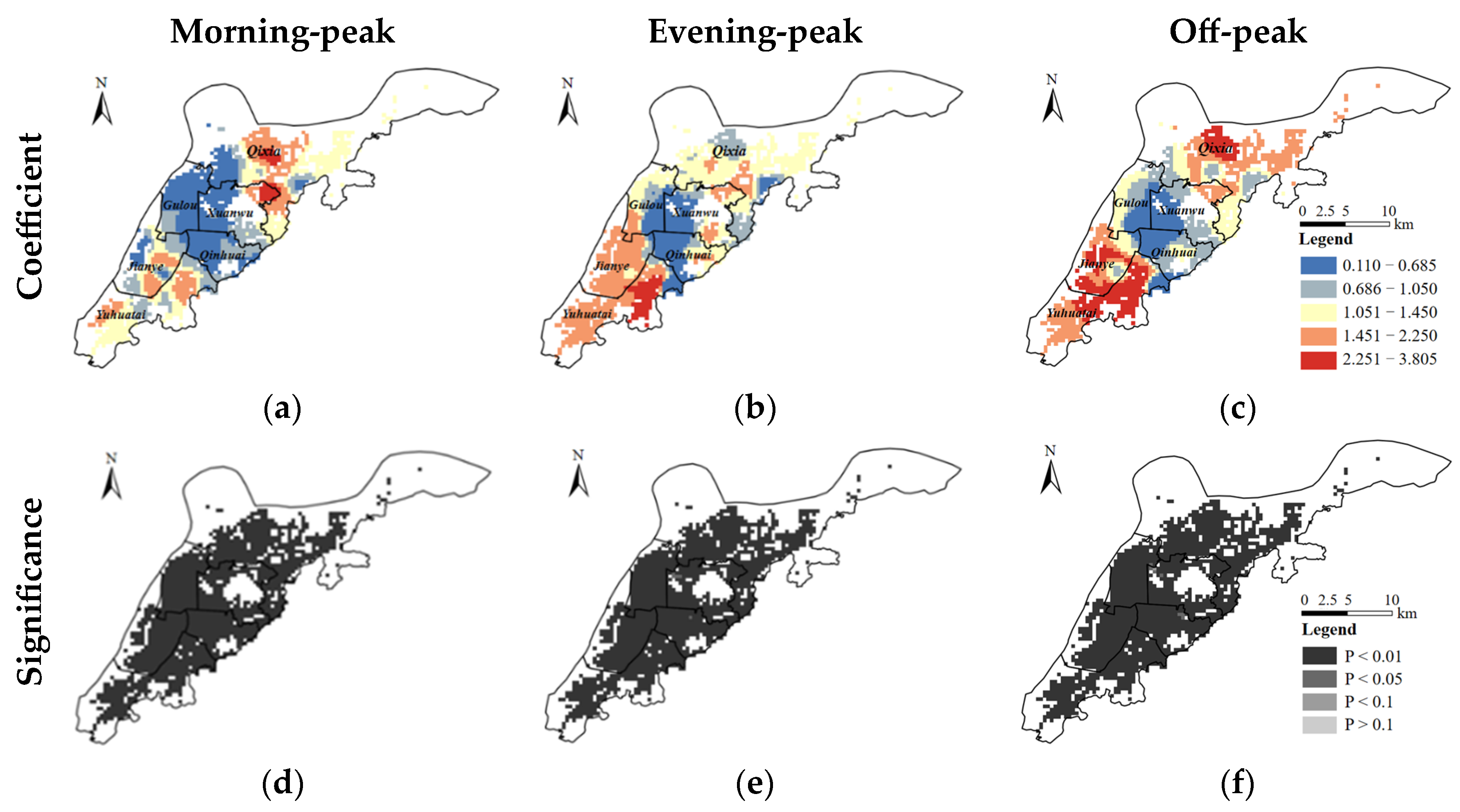
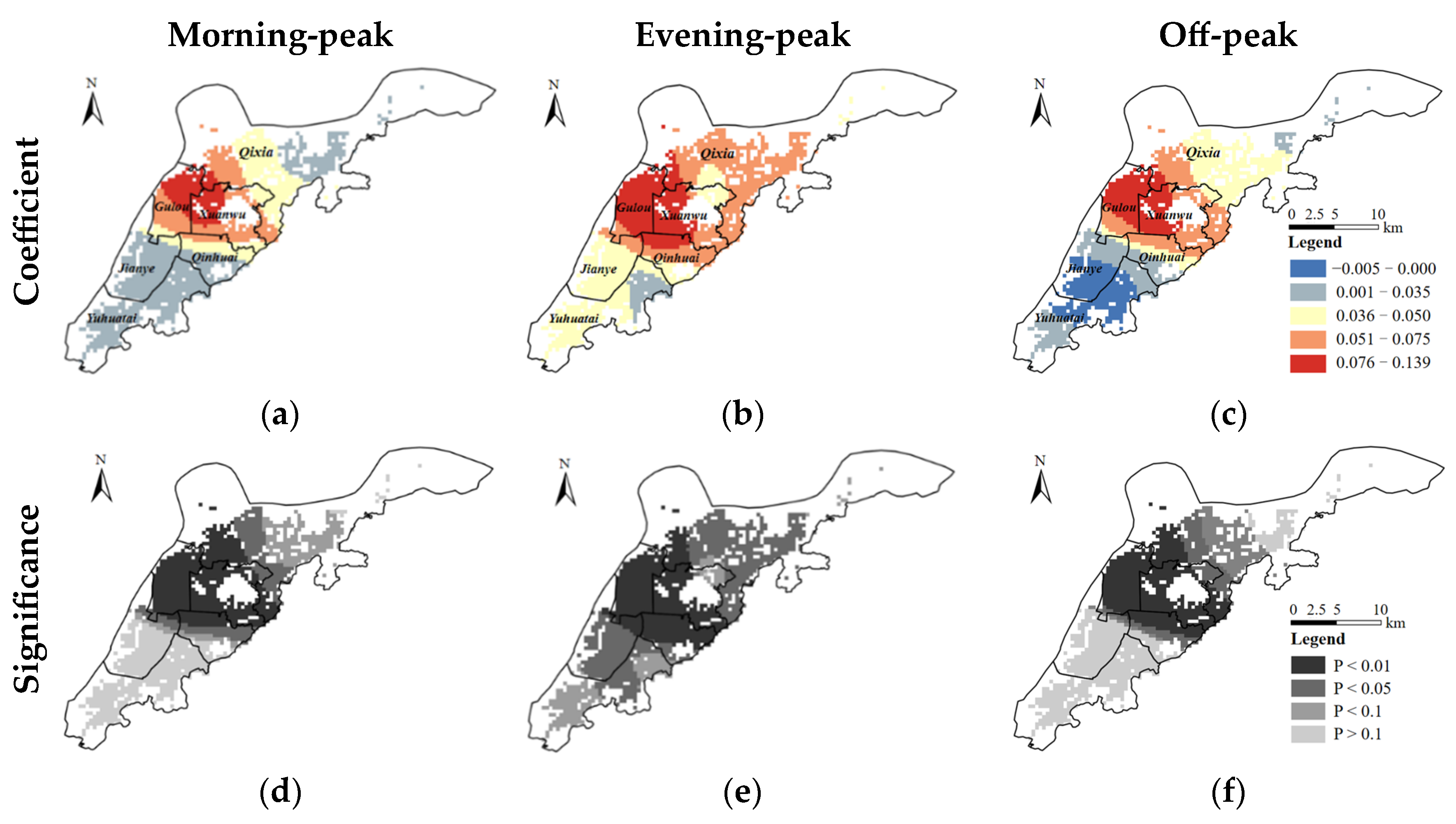
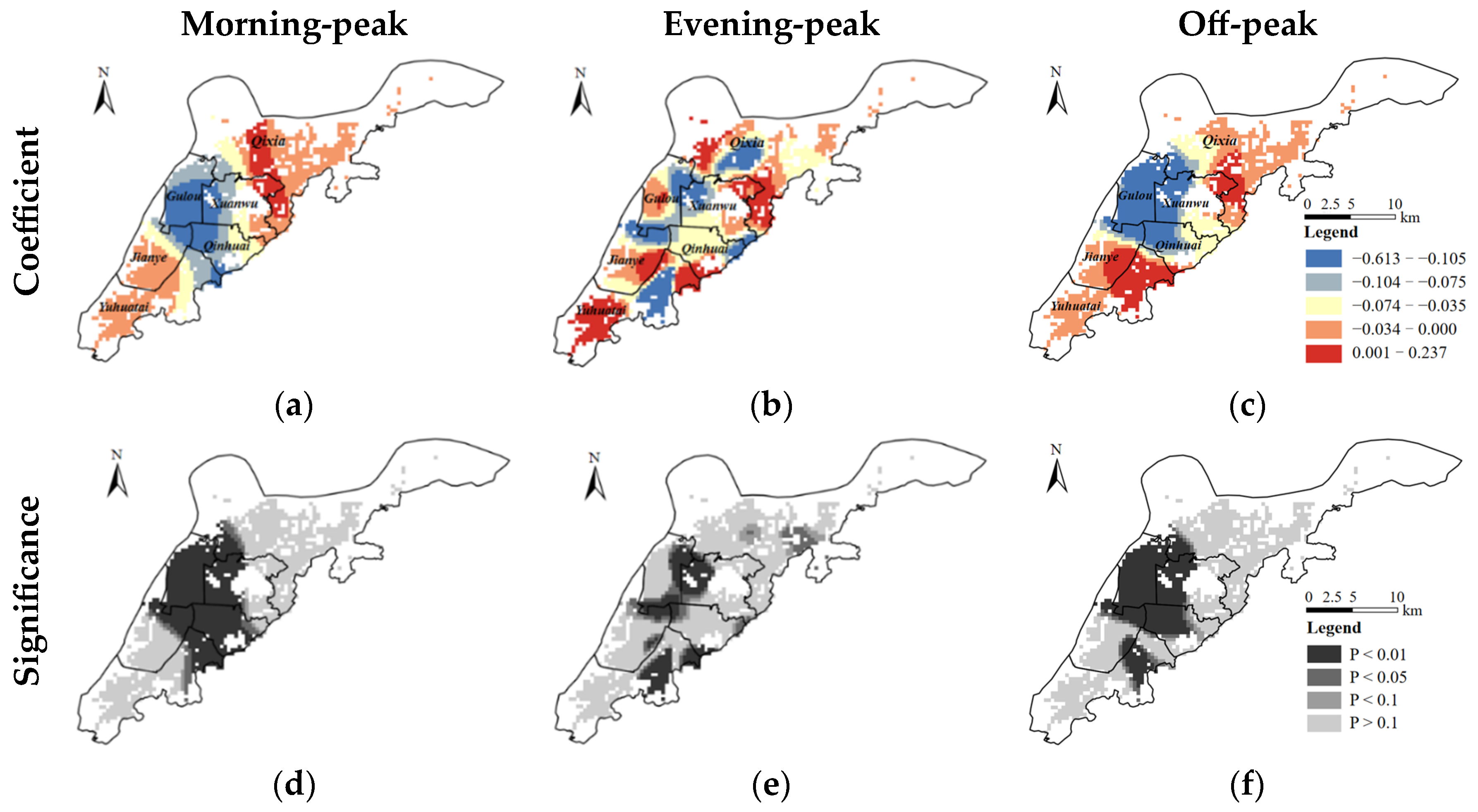
4.2. Regression Coefficients of MGWR

The MGWR results for ride-hailing ridership and its influencing factors at three different periods are presented in

Table 6. Regression coefficients of MGWR.

Variable	Mean	STD	Min	Median	Max
Morning-peak
Intercept	−0.175	0.43	−0.927	−0.179	0.935
Taxi ridership	1.053	0.552	0.162	0.998	2.690
Density
Population density	0.024	0.126	−0.162	0.029	0.308
Housing price	−0.001	0.001	−0.003	−0.001	0.001
Diversity
Land use mix	−0.011	0.002	−0.013	−0.012	−0.005
Design
Road density	0.040	0.022	0.011	0.037	0.084
Bike lane density	−0.050	0.046	−0.137	−0.034	0.034
Distance to transit
Bus stop density	0.009	0.002	0.006	0.008	0.012
Metro station density	0.101	0.239	−0.221	0.048	1.236
Distance to the nearest bus stop	−0.028	0.002	−0.03	−0.028	−0.025
Distance to the nearest metro station	−0.030	0.004	−0.037	−0.030	−0.024
Destination accessibility
Distance to CBD	−0.407	0.542	−2.225	−0.575	0.756
Evening-peak
Intercept	−0.008	0.14	−0.21	−0.007	0.263
Taxi ridership	1.283	0.618	0.11	1.274	3.805
Density
Population density	0.048	0	0.047	0.048	0.048
Housing price	−0.016	0.001	−0.019	−0.016	−0.015
Diversity
Land use mix	−0.015	0.005	−0.022	−0.017	−0.005
Design
Road density	0.061	0.026	0.032	0.055	0.139
Bike lane density	−0.047	0.113	−0.613	−0.041	0.237
Distance to transit
Bus stop density	0.016	0.001	0.014	0.015	0.017
Metro station density	0.081	0.126	−0.181	0.058	0.651
Distance to the nearest bus stop	−0.013	0.002	−0.016	−0.013	−0.010
Distance to the nearest metro station	−0.007	0.003	−0.012	−0.006	−0.004
Destination accessibility
Distance to CBD	−0.239	0.4	−2.614	−0.198	0.638
Off-peak
Intercept	−0.513	0.648	−1.853	−0.266	0.682
Taxi ridership	1.471	0.772	0.16	1.306	3.725
Density
Population density	0.055	0.098	−0.101	0.07	0.242
Housing price	−0.025	0.009	−0.035	−0.031	−0.004
Diversity
Land use mix	−0.084	0.154	−1.163	−0.018	0.102
Design
Road density	0.04	0.032	−0.005	0.04	0.1
Bike lane density	−0.043	0.074	−0.179	−0.031	0.222
Distance to transit
Bus stop density	0.016	0.001	0.013	0.016	0.017
Metro station density	0.038	0.065	−0.133	0.034	0.385
Distance to the nearest bus stop	−0.018	0	−0.019	−0.018	−0.016
Distance to the nearest metro station	0.038	0.017	−0.002	0.038	0.067
Destination accessibility
Distance to CBD	−0.91	0.912	−2.718	−1.482	0.404

. The utilization of MGWR allows for the exploration of spatial heterogeneity by providing varying coefficients across different spatial locations. Considering the spatial non-stationarity of the estimation coefficients, the minimum, median, mean, and maximum values of the coefficients are employed to assess the relationship between ride-hailing ridership and its influencing factors. The results highlight significant spatiotemporal heterogeneity in the link between ride-hailing ridership and its influencing factors. Taxi ridership has a positive impact on ride-hailing ridership, suggesting a cooperative relationship between taxis and ride-hailing. This result is in line with most existing studies [39]. Furthermore, road density exhibits a positive relationship with ride-hailing ridership, while bike lane density demonstrates a negative relationship. These contrasting effects indicate that higher road density contributes to increased ride-hailing ridership, whereas higher bike lane density is associated with reduced ride-hailing ridership. During the two peak periods, the effects of distance to the nearest bus stop and distance to the nearest metro station are both negative. Conversely, the effects of bus stop density and metro station density are positive; this has been confirmed by many studies [9]. These findings suggest that ride-hailing services complement public transit systems due to the dense areas of public transit stations tend to generate more travel demand, attracting online ride-hailing to provide travel services here. The relationship between distance to CBD and ride-hailing ridership is found to be non-stationary.

4.3. Spatiotemporal Variations in the Effects on Ride-Hailing Ridership

To explore the spatiotemporal variations in the effects of exogenous variables on ride-hailing ridership, we visualize the parameters of those variables that show heterogeneous effects on ride-hailing ridership at three periods. Hence, the spatiotemporal variations in the effects of taxi ridership, metro station density, distance to CBD, road density, and bike lane density on ride-hailing ridership are illustrated and discussed in this section.

Figure 3 illustrates the spatiotemporal variations in the effects of taxi ridership on ride-hailing ridership. Figure 3a–c are the taxi ridership coefficients of the morning peak, evening peak and off peak, Figure 3d–f are the significance of the three periods. The positive relationship between the two is consistent with the research conclusion of the literature [2], which may be due to the fact that, under the supervision of policies, the entry of ride-hailing into the market has promoted the reform of the taxi industry, and the two have evolved from a competitive landscape to a cooperative relationship. Based on the estimation results, although the effects of taxi ridership are always positive, the effect sizes vary across different spatial locations. The positive effects indicate that taxis show a cooperative relationship with ride-hailing. Notably, the effect sizes tend to gradually increase as they move from the urban center toward peripheral areas. This spatial pattern suggests that the impact of taxi ridership on ride-hailing ridership becomes more pronounced in the outskirts of the study area. In the junction of the Xuanwu, Qinhuai, Gulou, and Jianye districts, we observe that the local coefficients are the lowest among all grids. This finding can be attributed to the presence of the Central Business District (CBD) in Nanjing, specifically the Xinjiekou area, which offers high accessibility to public transit options and promotes better walkability. Consequently, the cooperative relationship between taxis and ride-hailing services might be weakened in these areas. Additionally, the coefficients are lower in the Gulou district relative to other districts. This result is reasonable because many universities are concentrated in the Gulou district, and university students tend to have stronger intentions to use ride-hailing services [8]. In the Jianye, Yuhuatai, and Qixia districts, we observe variations in the positive relationship between taxi ridership and ride-hailing ridership across the morning peak and evening peak periods. This discrepancy can be attributed to the distinct land use characteristics of each district. The Jianye district is primarily characterized by a blend of commercial and residential areas, while the Qixia and Yuhuatai districts serve as gathering places for firms with some residential zones. These diverse land uses result in differing intensities of commuting travel demand during the morning and evening peaks. It should be noted that taxis and ride-hailing show a stronger cooperative relationship during off-peak periods. This phenomenon can be attributed to the specific time chosen for the off-peak period in this study, which falls between 11:00 AM and 1:00 PM, typically coinciding with lunch breaks for companies, as well as residents’ dining time. The Jianye district, as a gathering place of commercial and residential lands, is densely populated, thus attracting online car-hailing and taxis to provide services. The Qixia and Yuhuatai districts are new urban areas for construction and development, lacking relevant entertainment and leisure places. In addition, the inadequate public transportation facilities in the two districts also increase the demand for taxis and ride-hailing.

Figure 4 and Figure 5 illustrate the spatiotemporal variations in the effects of road density and bike lane density on ride-hailing ridership. Figure 4a–c and Figure 5a–c are the road density and bike lane density coefficients of the morning peak, evening peak and off peak, Figure 4d–f and Figure 5d–f are the significance of the three periods. The findings indicate that, in general, the coefficients of road density gradually decrease from the urban center to peripheral areas. Compared with the Yuhuatai and Qixia districts, the local coefficients in the Gulou and Xuanwu districts are higher. This result may be explained by the fact that areas with higher road density tend to attract more people living and working and thus generate more travel demand. Tang et al. [40] also confirmed that high road density is associated with a high demand for ride-hailing. In contrast, bike lane density shows a significantly negative effect on ride-hailing ridership in the Gulou and Xuanwu districts, suggesting that increasing bike lane density may substitute for some ride-hailing demand. In some areas of the Yuhuaitai and Qixia districts, bike lane density shows a positive effect on ride-hailing ridership, suggesting that the current density of bike lanes is insufficient to meet residents’ travel demand.

As depicted in Figure 6, the parameters of metro station density exhibit spatial variations across the study area. Figure 6a–c are the metro station density coefficients of the morning peak, evening peak and off peak, Figure 6d–f are the significance of the three periods. Notably, in the Gulou and Xuanwu districts, metro station density demonstrates a positive effect on ride-hailing ridership overall. This implies that an increase in metro station density, particularly in areas with relatively low metro station density, may lead to a rise in ride-hailing demand in central urban areas. Residents in these districts may opt for a combination of ride-hailing and metro services for their commuting needs; they may take ride-hailing to metro stations nearby and then take the metro to work. As new urban areas for construction and development, the Yuhuatai district cannot provide sufficient public transit services to meet travel demand. Thus, metro station density shows positive local coefficients, especially at morning and evening peaks. One interesting thing is that areas around the university town in the Qixia district observe negative coefficients. This may be explained by the reason that university students are more likely to travel by metro due to its relatively lower travel costs.

Figure 7 presents the spatiotemporal variations in the effects of distance to CBD on ride-hailing ridership. Figure 7a–c are the distance to CBD coefficients of the morning peak, evening peak and off peak, Figure 7d–f are the significance of the three periods. In the Xuanwu, Qinhuai, Jianye, and Gulou districts, distance to CBD generally shows a negative effect on ride-hailing ridership. Moreover, the negative effects are stronger at the off-peak. All else equal, more intersection traffic lights and traffic congestion in central urban areas tend to lead to more delays, consequently leading to higher ride-hailing fees. Due to better public transit accessibility in these areas, people farther from CBD may travel by metro or bus instead of ride-hailing. Especially at off-peak, it is less crowded in public vehicles and may attract more travelers. By contrast, distance to CBD shows negative local coefficients in the Qixia and Yuhuaitai districts, which may be explained by poorer public transit services to a large extent.

5. Concluding Remarks

Although the links between the built environment and travel behavior have been widely researched, scant evidence has been provided on the heterogeneity in the links [31]. Only a few studies have attempted to identify the heterogeneous effect of the built environment on ride-hailing ridership [2,24]. However, existing studies tend to overlook the varying scales at which different built environment variables affect ride-hailing ridership. The MGWR model is employed to address the gap by exploring the spatiotemporal effects of the built environment on ride-hailing ridership based on ride-hailing order data of all TNCs in Nanjing. Additionally, the competitive and cooperative relationship between taxis and ride-hailing is also considered. The findings help researchers and policy practitioners better understand spatiotemporal patterns of ride-hailing ridership and its relationship with built environment characteristics and further promote contextualized policies for ride-hailing allocation and urban planning.

This study adds to the literature by revealing spatiotemporal heterogeneity in the determinants of ride-hailing ridership. The results of this study suggest that the MGWR model outperforms both the OLS and GWR models, highlighting the importance of utilizing different optimal bandwidths for each exogenous variable. In the MGWR model, the smallest bandwidths are observed for taxis during the morning peak, evening peak, and off-peak periods, confirming the spatial heterogeneity in the relationship between ride-hailing ridership and taxi ridership. As a result, we consider taxi ridership as a local variable in our analysis. The results suggest that metro station density, distance to CBD, road density, and bike lane density are considered local variables, whereas bus stop density, distance to the nearest bus stop, and distance to the nearest metro station are regarded as global variables. The bandwidths for population density and land use mix vary across three periods, and the spatial heterogeneity in these two variables is only observed during some specific periods.

The findings of this study reveal important insights into the relationships between various factors and ride-hailing ridership. Urban planners and policy makers can benefit from understanding the spatial and temporal heterogeneity of the impact of the built environment on ride-hailing ridership, and propose targeted improvement or optimization strategies according to local conditions. It provides a theoretical basis for optimizing the urban layout and promoting the coordinated development of ride-hailing, taxis, and public transit. Specifically, we observe a positive association between taxi ridership and ride-hailing ridership across all three periods, indicating a cooperative relationship between these two modes of transportation. Furthermore, this cooperative relationship is particularly pronounced in areas with limited access to adequate public transit services. Considering the low density of suburban travel, the cost of traditional cruise taxis is higher. Therefore, more ride-hailing can be configured in the suburbs to meet the travel needs of suburban residents. In addition, a higher road density is positively associated with more ride-hailing ridership, whereas bike lane density significantly decreases ride-hailing ridership in general. Only in some areas where the current density of bike lanes is insufficient to meet travel demand does bike lane density show a positive effect on ride-hailing demand. The parameters of metro station density vary across the study area. Distance to CBD generally shows a negative effect on ride-hailing ridership in central urban areas, whereas the effect is negative in areas where public transit services are inadequate. Policy makers should reduce ride-hailing services instead of short-distance trips by bicycle. In addition, the ride-hailing service provided by the central urban areas should be restricted, and other travel modes such as ride splitting, public transit, and non-motorized traffic should be developed to reduce the congestion caused by ride-hailing service.

Several limitations remain in this study. First, only data from Nanjing are used for this analysis. Future research could explore multiple cities with diverse characteristics to provide a more comprehensive understanding of the relationship between the built environment and ride-hailing ridership. Second, this analysis is conducted based on a cross-sectional research design. Aiming to understand the causal mechanisms between the built environment and ride-hailing ridership, more longitudinal data should be collected in future studies. Third, only the characteristics of the built environment and the impact of taxis on the demand for ride-hailing ridership are considered, and the relationship between ride-hailing and influencing factors may be disturbed by other potential factors [2]. In order to further clarify the above relationship, it is recommended to consider the interaction effect in further research. Fourth, the MGWR model used in this paper assumes that there is a linear or generalized linear relationship between the two, and the conclusions may have some deviations. The machine learning method has the advantage of not following the assumption of the linear relationships between variables in multivariate fitting, which is helpful in finding complex nonlinear relationships [41]. Finally, the application of artificial intelligence in dynamic mobility management can support demand management measures to achieve sustainable goals. Applying it to research on ride-hailing can better understand the service of ride-hailing [42].

References

1. Wang, S.; Noland, R.B. Variation in ride-hailing trips in Chengdu, China. Transp. Res. Part D Transp. Environ. 2021, 90, 102596. [Google Scholar] [CrossRef]
2. Liu, F.; Gao, F.; Yang, L.; Han, C.; Hao, W.; Tang, J. Exploring the spatially heterogeneous effect of the built environment on ride-hailing travel demand: A geographically weighted quantile regression model. Travel Behav. Soc. 2022, 29, 22–33. [Google Scholar] [CrossRef]
3. The Online Car-Hailing Supervision Information Interaction System Released the Basic Operation of the Online Car-Hailing Industry in May 2023. Available online: https://www.mot.gov.cn/fenxigongbao/yunlifenxi/202306/t20230613_3845580.html (accessed on 13 June 2023).
4. Gehrke, S.R. Uber service area expansion in three major American cities. J. Transp. Geogr. 2020, 86, 102752. [Google Scholar] [CrossRef]
5. Rayle, L.; Dai, D.; Chan, N.; Cervero, R.; Shaheen, S. Just a better taxi? A survey-based comparison of taxis, transit, and ridesourcing services in San Francisco. Transp. Policy 2016, 45, 168–178. [Google Scholar] [CrossRef]
6. Yu, H.; Peng, Z.-R. Exploring the spatial variation of ridesourcing demand and its relationship to built environment and socioeconomic factors with the geographically weighted Poisson regression. J. Transp. Geogr. 2019, 75, 147–163. [Google Scholar] [CrossRef]
7. Qian, X.; Ukkusuri, S.V. Spatial variation of the urban taxi ridership using GPS data. Appl. Geogr. 2015, 59, 31–42. [Google Scholar] [CrossRef]
8. Lee, S.; Lee, W.; Vogt, C.A.; Zhang, Y. A comparative analysis of factors influencing millennial travellers’ intentions to use ride-hailing. Inf. Technol. Tour. 2021, 23, 133–157. [Google Scholar] [CrossRef]
9. Sabouri, S.; Park, K.; Smith, A.; Tian, G.; Ewing, R. Exploring the influence of built environment on Uber demand. Transp. Res. Part D Transp. Environ. 2020, 81, 102296. [Google Scholar] [CrossRef]
10. Wang, D.; Miwa, T.; Morikawa, T. Interrelationships between traditional taxi services and online ride-hailing: Empirical evidence from Xiamen, China. Sustain. Cities Soc. 2022, 83, 103924. [Google Scholar] [CrossRef]
11. Li, X.; Xu, J.; Du, M.; Liu, D.; Kwan, M.-P. Understanding the spatiotemporal variation of ride-hailing orders under different travel distances. Travel Behav. Soc. 2023, 32, 100581. [Google Scholar] [CrossRef]
12. An, R.; Wu, Z.; Tong, Z.; Qin, S.; Zhu, Y.; Liu, Y. How the built environment promotes public transportation in Wuhan: A multiscale geographically weighted regression analysis. Travel Behav. Soc. 2022, 29, 186–199. [Google Scholar] [CrossRef]
13. Ghaffar, A.; Mitra, S.; Hyland, M. Modeling determinants of ridesourcing usage: A census tract-level analysis of Chicago. Transp. Res. Part C Emerg. Technol. 2020, 119, 102769. [Google Scholar] [CrossRef]
14. Deka, D.; Fei, D. A comparison of the personal and neighborhood characteristics associated with ridesourcing, transit use, and driving with NHTS data. J. Transp. Geogr. 2019, 76, 24–33. [Google Scholar] [CrossRef]
15. Tang, B.-J.; Li, X.-Y.; Yu, B.; Wei, Y.-M. How app-based ride-hailing services influence travel behavior: An empirical study from China. Int. J. Sustain. Transp. 2019, 14, 554–568. [Google Scholar] [CrossRef]
16. Tirachini, A.; Gomez-Lobo, A. Does ride-hailing increase or decrease vehicle kilometers traveled (VKT)? A simulation approach for Santiago de Chile. Int. J. Sustain. Transp. 2019, 14, 187–204. [Google Scholar] [CrossRef]
17. He, Z. Portraying ride-hailing mobility using multi-day trip order data: A case study of Beijing, China. Transp. Res. Part A Pol. Pract. 2021, 146, 152–169. [Google Scholar] [CrossRef]
18. Du, M.; Li, X.; Kwan, M.-P.; Yang, J.; Liu, Q. Understanding the Spatiotemporal Variation of High-Efficiency Ride-Hailing Orders: A Case Study of Haikou, China. ISPRS Int. J. Geo-Inf. 2022, 11, 42. [Google Scholar] [CrossRef]
19. Zhang, B.; Chen, S.; Ma, Y.; Li, T.; Tang, K. Analysis on spatiotemporal urban mobility based on online car-hailing data. J. Transp. Geogr. 2020, 82, 102568. [Google Scholar] [CrossRef]
20. Yu, H.; Peng, Z.-R. The impacts of built environment on ridesourcing demand: A neighbourhood level analysis in Austin, Texas. Urban Stud. 2019, 57, 152–175. [Google Scholar] [CrossRef]
21. Mwombeki, F.A. Influencing Attributes on Revenue Growth: An Empirical Analysis from SMEs in Tanzania. JAFAS 2023, 9, 199–216. [Google Scholar] [CrossRef]
22. Mashamba, T. Determinates of Commercial Banks Liquidity: Internal Factor Analysis. JCGIRM 2014, 1, 112–131. [Google Scholar] [CrossRef]
23. Dean, M.D.; Kockelman, K.M. Spatial variation in shared ride-hail trip demand and factors contributing to sharing: Lessons from Chicago. J. Transp. Geogr. 2021, 91, 102944. [Google Scholar] [CrossRef]
24. Zheng, Z.; Zhang, J.; Zhang, L.; Li, M.; Rong, P.; Qin, Y. Understanding the impact of the built environment on ride-hailing from a spatio-temporal perspective: A fine-scale empirical study from China. Cities 2022, 126, 103706. [Google Scholar] [CrossRef]
25. Gan, Z.; Yang, M.; Feng, T.; Timmermans, H.J.P. Examining the relationship between built environment and metro ridership at station-to-station level. Transp. Res. Part D Transp. Environ. 2020, 82, 102332. [Google Scholar] [CrossRef]
26. Fotheringham, A.S.; Yang, W.; Kang, W. Multiscale Geographically Weighted Regression (MGWR). Ann. Am. Assoc. Geogr. 2017, 107, 1247–1265. [Google Scholar] [CrossRef]
27. Mansour, S.; Al Kindi, A.; Al-Said, A.; Al-Said, A.; Atkinson, P. Sociodemographic determinants of COVID-19 incidence rates in Oman: Geospatial modelling using multiscale geographically weighted regression (MGWR). Sustain. Cities Soc. 2021, 65, 102627. [Google Scholar] [CrossRef] [PubMed]
28. Zhao, G.; Li, Z.; Shang, Y.; Yang, M. How Does the Urban Built Environment Affect Online Car-Hailing Ridership Intensity among Different Scales? Int. J. Environ. Res. Public Health 2022, 19, 5325. [Google Scholar] [CrossRef] [PubMed]
29. Yu, B.; Lian, T.; Huang, Y.; Yao, S.; Ye, X.; Chen, Z.; Yang, C.; Wu, J. Integration of nighttime light remote sensing images and taxi GPS tracking data for population surface enhancement. Int. J. Geogr. Inf. Sci. 2018, 33, 687–706. [Google Scholar] [CrossRef]
30. Li, T.; Jing, P.; Li, L.; Sun, D.; Yan, W. Revealing the Varying Impact of Urban Built Environment on Online Car-Hailing Travel in Spatio-Temporal Dimension: An Exploratory Analysis in Chengdu, China. Sustainability 2019, 11, 1336. [Google Scholar] [CrossRef]
31. Ewing, R.; Cervero, R. Travel and the Built Environment. J. Am. Plann. Assoc. 2010, 76, 265–294. [Google Scholar] [CrossRef]
32. Pohlmann, J.T.; Leitner, D.W. A comparison of ordinary least squares and logistic regression. Ohio J. Sci. 2003, 103, 118–125. [Google Scholar]
33. Cheng, L.; Shi, K.; De Vos, J.; Cao, M.; Witlox, F. Examining the spatially heterogeneous effects of the built environment on walking among older adults. Transp. Policy 2021, 100, 21–30. [Google Scholar] [CrossRef]
34. Bi, H.; Ye, Z.; Wang, C.; Chen, E.; Li, Y.; Shao, X. How Built Environment Impacts Online Car-Hailing Ridership. Transp. Res. Rec. J. Transp. Res. Board 2020, 2674, 745–760. [Google Scholar] [CrossRef]
35. Mollalo, A.; Vahedi, B.; Rivera, K.M. GIS-based spatial modeling of COVID-19 incidence rate in the continental United States. Sci. Total Environ. 2020, 728, 138884. [Google Scholar] [CrossRef] [PubMed]
36. Wu, T.; Zhou, L.; Jiang, G.; Meadows, M.E.; Zhang, J.; Pu, L.; Wu, C.; Xie, X. Modelling Spatial Heterogeneity in the Effects of Natural and Socioeconomic Factors, and Their Interactions, on Atmospheric PM2.5 Concentrations in China from 2000–2015. Remote Sens. 2021, 13, 2152. [Google Scholar] [CrossRef]
37. Song, J.; Yu, H.; Lu, Y. Spatial-scale dependent risk factors of heat-related mortality: A multiscale geographically weighted regression analysis. Sustain. Cities Soc. 2021, 74, 103159. [Google Scholar] [CrossRef]
38. Feuillet, T.; Commenges, H.; Menai, M.; Salze, P.; Perchoux, C.; Reuillon, R.; Kesse-Guyot, E.; Enaux, C.; Nazare, J.A.; Hercberg, S.; et al. A massive geographically weighted regression model of walking-environment relationships. J. Transp. Geogr. 2018, 68, 118–129. [Google Scholar] [CrossRef]
39. Vega-Gonzalo, M.; Aguilera-García, Á.; Gomez, J.; Vassallo, J.M. Traditional taxi, e-hailing or ride-hailing? A GSEM approach to exploring service adoption patterns. Transportation 2023. [Google Scholar] [CrossRef]
40. Tang, J.; Gao, F.; Liu, F.; Zhang, W.; Qi, Y. Understanding Spatio-Temporal Characteristics of Urban Travel Demand Based on the Combination of GWR and GLM. Sustainability 2019, 11, 5525. [Google Scholar] [CrossRef]
41. Ji, S.; Wang, X.; Lyu, T.; Liu, X.; Wang, Y.; Heinen, E.; Sun, Z. Understanding cycling distance according to the prediction of the XGBoost and the interpretation of SHAP: A non-linear and interaction effect analysis. J. Transp. Geogr. 2022, 103, 103414. [Google Scholar] [CrossRef]
42. Cirianni, F.M.M.; Comi, A.; Quattrone, A. Mobility Control Centre and Artificial Intelligence for Sustainable Urban Districts. Information 2023, 14, 581. [Google Scholar] [CrossRef]
Figure 1. Study area.
Applsci 14 00142 g001
Figure 2. Spatiotemporal distributions of ride-hailing ridership and taxi ridership.
Applsci 14 00142 g002
Figure 3. Spatiotemporal variations in the coefficients of taxi ridership.
Applsci 14 00142 g003
Figure 4. Spatiotemporal variations in the coefficients of road density.
Applsci 14 00142 g004
Figure 5. Spatiotemporal pattern in the coefficients of bike lane density.
Applsci 14 00142 g005
Figure 6. Spatiotemporal variations in the coefficients of metro station density.
Applsci 14 00142 g006
Figure 7. Spatiotemporal variations in the coefficients of distance to CBD.
Applsci 14 00142 g007