Computational Accuracy and Efficiency of Room Acoustics Simulation Using a Frequency Domain FEM with Air Absorption: 2D Study

Abstract

Recently, to simulate sound propagation inside architectural spaces at high frequencies, the application of computationally expensive wave-based numerical methods to room acoustics simulation is increasing gradually. Generally, standard room acoustics simulations in the frequency domain are performed based on the lossless Helmholtz equation. However, for acoustics simulation at high frequencies, consideration of the sound attenuation effect caused by air absorption is an aspect to increase the reliability of predictions. Although a simple approach based on the lossy Helmholtz equation is available to include the air absorption effect in the frequency domain, its accuracy and efficiency are still not discussed well. This paper presents an accuracy and efficiency estimation of FEM based on the lossy Helmholtz equation via two numerical problems in two dimensions: a plane wave propagation problem up to 20 kHz in a long duct with 1 km length and a sound propagation problem in a real-scale office up to 6 kHz. Results revealed that the lossy Helmholtz equation-based FEM can include the air absorption effect accurately up to 20 kHz. Moreover, a possibility of providing a higher computational efficiency at higher frequencies is suggested when the magnitude of the pure-tone sound attenuation coefficient is large.

1. Introduction

Computational acoustics simulation methods [1] are indispensable tools for designing room acoustics in various architectural spaces and acoustic virtual reality applications [2]. Two simulation methods, called geometrical acoustic methods and wave-based numerical methods, are available, and they have unique strengths and shortcomings. The former is already a general-purpose method, and the latter is gradually gaining interest thanks to recent developments in computer technology. Geometrical acoustic methods [3], such as acoustic ray tracing [4], beam tracing, and the image source method [5], are widely used practical acoustic simulation tools with high computational efficiency. The geometrical acoustic methods model, sound propagation as ray propagation, and wave phenomena such as diffraction and interference are not addressed accurately. Therefore, efforts to improve the accuracy have been undertaken. For example, the phase beam tracing method [6,7,8,9] can include phase information essential for dealing with the interference effect and phase shift on reflection at boundaries.

On the other hand, room acoustic simulations with wave-based numerical methods, such as the finite difference time-domain (FDTD) method [10,11,12,13,14], finite element method (FEM) [15,16,17,18,19,20], and boundary element method (BEM) [21,22,23,24,25], have become applicable for the accurate prediction of indoor sound environments. Compared to practical geometrical room acoustic simulations using ray tracing methods [3], wave-based room acoustic simulations have attractive benefits, providing a reliable prediction by solving the partial differential equations of wave phenomena, such as the wave equation in the time-domain analysis and the Helmholtz equation in the frequency-domain analysis. However, because wave-based room acoustics simulation requires vast computational times for practical-sized rooms, many researchers have been striving to develop computationally efficient wave-based methods. Through outcomes established from their studies, some recent works [18,19,20] have demonstrated that recently developed wave-based room acoustic solvers with FEM in the time domain can predict indoor acoustics up to 6 kHz in small room spaces, such as classrooms and meeting rooms, within practical computational times. Moreover, they have shown a fundamental effectiveness as a virtual indoor sound environment creation tool for virtual reality applications. It is also worth mentioning that a hybrid technique [26,27] that tries to combine the strength of geometrical acoustic methods and wave-based numerical methods is an attractive direction for room acoustics simulation. It can enhance accuracy at low frequencies while keeping computational efficiency. Among the above three directions on room acoustics simulation, i.e., the use of geometrical acoustic methods, wave-based numerical methods, and their hybrid techniques, the present paper specifically focuses on wave-based numerical methods using FEM.

Apart from developing highly efficient methods on wave-based numerical methods, an essential key to reliable room acoustics prediction is the use of accurate sound attenuation models for acoustic materials installed in spaces and sound wave propagation in the air. Acoustic materials such as porous and resonant absorbers [28,29], which are common sound-absorbing materials for room acoustics control, have frequency-dependent and incident-angle-dependent sound absorption characteristics. Impedance boundary conditions, which use theoretically computed or measured complex-valued specific acoustic impedance of materials, are used to describe the frequency dependence of acoustic properties of local-reaction materials. Impedance tube measurements described in ISO 10534-2 [30] and in-situ measurements [31] are available as measurement-based approaches for this purpose. The transfer matrix method [32] is a theoretical method of computing the specific acoustic impedance of materials. Extended-reaction models that solve the partial differential equations of materials are used to describe the incident-angle-dependent absorption characteristics. A simple equivalent fluid model based on the lossy Helmholtz equation and the poroelastic material model based on the Biot theory have been used [33,34,35]. By contrast, standard room acoustics simulation usually solves the lossless wave equation and Helmholtz equation for sound propagation in the air inside rooms. Their lossless equations do not address the sound attenuation effects of air absorption caused by viscothermal effects and relaxation processes. However, considering the current situation in the applicable range of wave-based room-acoustics simulation to high frequencies, wave-based room acoustics simulation including air absorption might be an aspect for increasing their predictive reliability.

Some approaches can be used to include the air absorption effect. A recent report of the literature [36] proposes a low pass filter-based post-processing approach that uses a cascade of three time-varying IIR filters, approximating the air absorption model described in ISO 9613-1 [37]. The air absorption effect is added by filtering impulse responses without air absorption with time-varying IIR filters. For one earlier study [38], FIR filter-based approximation of air absorption was used to study the audibility of the dispersion error in a room acoustic FDTD solver. As a physically based approach for time-domain analysis, an acoustic FDTD solver discretized on Stokes’ equation has been used to include the air absorption effect caused by relaxation absorption from oxygen molecules, which has a dominant role in sound attenuation at high frequencies within the audible frequency range [39]. A time-domain wave-based room acoustics model, including viscothermal and relaxation effects in air, has also been proposed with corresponding FDTD discretization schemes [40]. Stokes’ equation can be reduced to the lossy Helmholtz equation with a complex-valued wave number assuming time-harmonic sound pressure [41]. Therefore, for frequency-domain analysis, a simple approach that solves the lossy Helmholtz equation with the pure-tone attenuation coefficient describing sound attenuation because of classical absorption and molecular relaxation absorption is available to implement air absorption effects. The study described herein specifically examines the simple lossy Helmholtz equation approach in the frequency domain. As described previously, the lossy Helmholtz equation with a complex wave number has been used to model viscothermal dissipation of sound-absorbing materials such as porous and resonator absorbers as equivalent fluids [42,43,44,45,46,47,48,49]. Nevertheless, how the lossy Helmholtz equation approach models air absorption effects accurately and efficiently has not been discussed adequately in earlier reports of the relevant literature.

This report of our study is intended to demonstrate, via two numerical problems, the accuracy and computational efficiency of the lossy Helmholtz equation-based FEM to include air absorption effects. One problem is long-range plane wave propagation in a long duct for an accuracy assessment up to 20 kHz. Another is a sound propagation problem in a real-scale 2D office for computational efficiency estimation. As a salient contribution of this study, we will reveal empirically that lossy Helmholtz equation-based FEM in the frequency domain has attractive features in terms of computational efficiency for room acoustics simulation at high frequencies. The structure of this paper is as follows. Section 2 presents the lossy Helmholtz equation approach, with the pure-tone attenuation coefficient based on the ISO 9613-1 model to add air absorption effects to FEM in the frequency domain. Then, Section 3 presents accuracy assessment results obtained for the lossy Helmholtz equation-based FEM via the long-range plane wave propagation problem in a long duct. In Section 4, the computational efficiency of the lossy Helmholtz equation-based FEM is demonstrated via a real-scale 2D office problem. Section 5 concludes the discussion presented herein.

2. Theory

2.1. Lossy Helmholtz Equation Approach

We consider the following plane wave propagation model with the air absorption effect described in ISO 9613-1 [37] as

$$p(x,t)=p_{\mathrm{i}}{\mathrm{e}}^{-\alpha x},$$

(1)

where the pure-tone sound pressure at time t and at distance x is represented by $p(x,t)$. In this model, a plane wave $p_{\mathrm{i}}$ exponentially attenuates against the propagation distance according to the pure-tone sound attenuation coefficient $\alpha$ [Np], which describes the attenuation per unit length attributable to the classical absorption and molecular relaxation absorption. Note that Np represents a unit called $\mathit{neper}$, which has a relation 1 [Np] = 20/ln(10) [dB]. Plane wave $p_{\mathrm{i}}$ takes the form of

$$p_{\mathrm{i}}={\mathrm{e}}^{-\mathrm{j}(k_{0}x-\omega t)},$$

(2)

with the wave number of lossless air $k_0=\omega /c_0$, where $\omega$ is the angular frequency, and where $c_0$ is the speed of sound. With the plane wave form, Equation (1) can be expressed as

$$p(x,t)={\mathrm{e}}^{-\mathrm{j}\tilde{k}x}{\mathrm{e}}^{\mathrm{j}\omega t},$$

(3)

where $\tilde{k}$ denotes the complex wavenumber given as $\tilde{k}=k_0-\mathrm{j}\alpha$. Based on this plane wave propagation model with $\tilde{k}$, the air absorption effect is incorporated into the acoustic simulation in the frequency domain as the lossy Helmholtz equation approach, which solves the following equation as

$$({\nabla }^2+{\tilde{k}}^2)\widehat{p}(\mathit{r},\omega )=-\mathrm{j}\omega {\rho }_0\widehat{q}\left(\omega \right)\delta (\mathit{r}-{\mathit{r}}_{\mathrm{s}}),$$

(4)

where $\widehat{p}(\mathit{r},\omega )$ stands for the complex-valued sound pressure at the position $\mathit{r}$ in the Cartesian coordinate system, ${\rho }_0$ represents the air density, $\widehat{q}\left(\omega \right)$ signifies the volume source strength density, and $\delta$ expresses the delta function. The position vector at a source point is represented by ${\mathit{r}}_{\mathrm{s}}$.

2.2. Calculation of the Pure-Tone Sound Attenuation Coefficient

The pure-tone sound attenuation coefficient $\alpha$ is a frequency-dependent value determined by four variables: the sound frequency, air temperature, air humidity, and atmospheric pressure. As physical mechanisms of air absorption, $\alpha$, which is defined by a unit [dB/m], includes four absorption mechanisms as

$$\alpha ={\alpha }_{\mathrm{cl}}+{\alpha }_{\mathrm{rot}}+{\alpha }_{\mathrm{vib},\mathrm{O}}+{\alpha }_{\mathrm{vib},\mathrm{N}},$$

(5)

where ${\alpha }_{\mathrm{cl}}$ represents the classical absorption by the transport processes of classical physics, ${\alpha }_{\mathrm{rot}}$ signifies the molecular absorption by rotational relaxation, and ${\alpha }_{\mathrm{vib},\mathrm{O}}$ and ${\alpha }_{\mathrm{vib},\mathrm{N}}$, respectively, denote the molecular absorption by vibrational relaxation of oxygen and nitrogen. All numerical experiments conducted for this study use the calculation procedure described in Annex A in ISO 9613-1 [37] to compute the four terms in Equation (5).

2.3. Spatial Discretization with Finite Elements

The inhomogeneous lossy Helmholtz equation of Equation (4) is solved numerically with standard Galerkin FEM discretization to compute the complex-valued sound pressure, including the air absorption effect. The weak form of Equation (4) is

$${\int }_{\mathrm{\Omega }}\nabla \chi {(\nabla \widehat{p})}^{\mathrm{T}}\mathrm{d}\mathrm{\Omega }-{\int }_{\mathrm{\Gamma }}\chi \frac{\partial \widehat{p}}{\partial n}\mathrm{d}\mathrm{\Gamma }-{\tilde{k}}^2{\int }_{\mathrm{\Omega }}\chi \widehat{p}\mathrm{d}\mathrm{\Omega }=\mathrm{j}\omega {\rho }_0\widehat{q}{\int }_{\mathrm{\Omega }}\chi \delta (\mathit{r}-{\mathit{r}}_{\mathrm{s}})\mathrm{d}\mathrm{\Omega },$$

(6)

where $\mathrm{\Omega }$ denotes the domain, $\mathrm{\Gamma }$ stands for the boundary of $\mathrm{\Omega }$, and $\chi$ is the weight function. In FEM, sound pressure $\widehat{p}\left(\mathit{r}\right)$ at point $\mathit{r}$ within element ${\mathrm{\Omega }}_e$ is approximated by a linear combination of two vectors $\mathit{N}$ and ${\mathit{p}}_e$ as $\widehat{p}\left(\mathit{r}\right)=\mathit{N}{\mathit{p}}_e$, where $\mathit{N}$ and ${\mathit{p}}_e$, respectively, denote the shape function vector and nodal sound pressure vector. The following Lagrange polynomials are used for $\mathit{N}$:

$$l_a\left({\xi }^m\right)=\prod _{b=1,(b\ne a)}^{p^{{\xi }^m}+1}\frac{{\xi }^m-{\xi }_b^m}{{\xi }_a^m-{\xi }_b^m},$$

(7)

where $l_a\left({\xi }^m\right)$ is the Lagrange polynomial for the ${\xi }^m$ direction in the local coordinate system. Subscript a denotes the node location, ${\xi }_a^m$ is the corresponding local coordinate, $p^{{\xi }^m}+1$ is the node number used for FE approximation, and $p^{{\xi }^m}$ is the order of the polynomial. This study specifically addresses 2D room acoustics simulation discretized using four-node linear quadrilateral elements (Q4s) with $p^{{\xi }^1}=p^{{\xi }^2}=1$. In this case, the shape function vector $N_i(i=1,2,3,4)$ components are given as

$$N_i({\xi }^1,{\xi }^2)=l_a\left({\xi }^1\right)l_a\left({\xi }^2\right).$$

(8)

With Q4s, $\mathit{N}$ and ${\mathit{p}}_e$ are given, respectively, as $\mathit{N}=[N_1,N_2,N_3,N_4]$ and ${\mathit{p}}_e={[\widehat{p_1},\widehat{p_2},\widehat{p_3},\widehat{p_4}]}^{\mathrm{T}}$. The same function form as $\widehat{p}\left(\mathit{r}\right)$ is applied to the weight function for the spatial discretization of Equation (6). Using sound field approximation within ${\mathrm{\Omega }}_e$ and inserting three boundary conditions (rigid boundary ${\mathrm{\Gamma }}_r$, vibration boundary ${\mathrm{\Gamma }}_v$, and impedance boundary ${\mathrm{\Gamma }}_a$ conditions) to Equation (6) leads to the following linear system of equations as

$$(\mathit{K}-{\tilde{k}}^2\mathit{M}+\mathrm{j}\omega \mathit{C})\mathit{p}=\mathit{f},$$

(9)

where $\mathit{K}$, $\mathit{M}$, and $\mathit{C}$, respectively, represent the stiffness, mass, and dissipation matrices, and where $\mathit{f}$ is the external force vector. Sound pressure vector $\mathit{p}$ composed of complex-valued sound pressure at all nodes is computed by solving Equation (9) using a linear system solver, such as a direct solver [50] or iterative solver [51]. Since the coefficient matrix of Equation (9) becomes a complex-valued sparse symmetric matrix with many zero components, the use of sparse linear system solvers is helpful to conserve memory when predicting a large-scale sound field with vastly numerous degrees of freedom (DOF). This report uses two sparse linear system solvers. For the accuracy assessment in Section 3, a sparse direct solver called PARDISO (included in the Intel Math Kernel Library) is used because sparse direct solvers produce accurate solutions. Additionally, an iterative solver called the CSQMOR method [52] with a diagonal scaling preconditioning is used as a linear system solver for the office problem in Section 4 for efficiency estimations because iterative solvers can have the potential to solve large-scale problems with lower memory usage and with less computational time than direct solvers. The convergence tolerance is set as 10${}^{-4}$. In iterative solvers, the setup of an arbitrary initial value affects their convergence to some degree (Section S2 of the Supplemental Material in [20] provides additional details.). The study described herein uses a zero initial value for the first pure-tone sound analysis and the previous frequency’s solution value for the remaining pure-tone sound analyses.

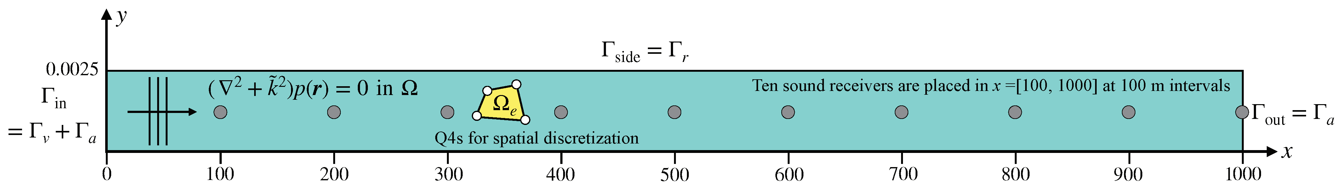
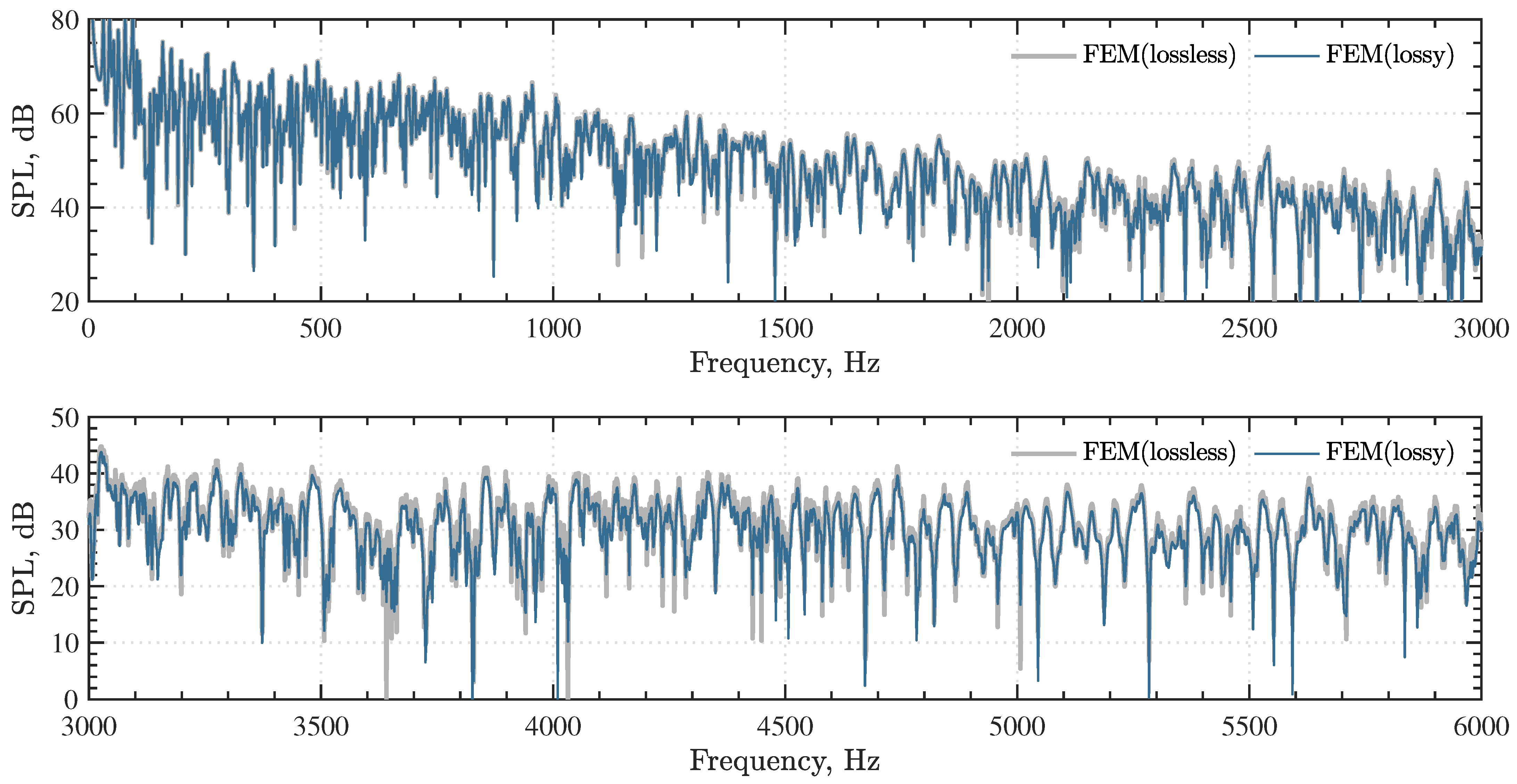
3. Accuracy Assessment with 2D Long Duct Problem

3.1. Outline of the Problem

This section presents an examination of the accuracy of lossy Helmholtz equation-based FEM to include the air absorption effect. To this end, as a benchmark problem, we propose a plane wave propagation problem in a 2D long duct with a 1000 m length. Figure 1 portrays the geometry of the 2D duct. Multi-frequency analyses using the lossy Helmholtz equation-based FEM and lossless Helmholtz equation-based FEM were performed, respectively, to calculate frequency responses at ten receiving points placed at $x=[100,1000]$ with 100 m intervals in the duct. The calculation was performed at 1 Hz to 20 kHz with 1 Hz intervals. The lossless Helmholtz equation approach solves the Helmholtz equation with real-valued wave number $k_0$ to compute frequency responses without the air absorption effects. Attenuation levels $L_{\mathrm{att}.}^{fem}$ attributable to air absorption were computed further as the difference of frequency responses between the lossy and the lossless Helmholtz equation approaches:

$$L_{\mathrm{att}.}^{fem}(\mathit{r},\omega )=|L_{\mathrm{lossy}}(\mathit{r},\omega )-L_{\mathrm{lossless}}(\mathit{r},\omega )|\left[\mathrm{dB}\right].$$

(10)

Therein, $L_{\mathrm{lossy}}(\mathit{r},\omega )$ and $L_{\mathrm{lossless}}(\mathit{r},\omega )$, respectively, denote the sound pressure levels computed using the lossy and lossless Helmholtz equation approaches. Then, the numerical attenuation levels $L_{\mathrm{att}.}^{fem}$ were compared with the theoretical ones $L_{\mathrm{att}.}^{theory}$ computed using the pure-tone sound attenuation coefficient in ISO 9613-1. For a quantitative evaluation of accuracy, we define the relative error $e_{\mathrm{att}.}$ in the attenuation levels as

$$e_{\mathrm{att}.}(\mathit{r},\omega )=\frac{L_{\mathrm{att}.}^{fem}(\mathit{r},\omega )}{L_{\mathrm{att}.}^{theory}(\mathit{r},\omega )}\times 100[\%].$$

(11)

This study evaluated the $e_{\mathrm{att}.}$ at the most distant receiver $\mathit{r}=(1000,0)$. Regarding the boundary conditions, the duct inlet ${\mathrm{\Gamma }}_{\mathrm{in}}$ in Figure 1 has a vibration boundary ${\mathrm{\Gamma }}_v$ with vibration velocity of 1.0 m/s, radiating a plane wave. To consider only the progressive wave in the positive x direction, the duct inlet ${\mathrm{\Gamma }}_{\mathrm{in}}$ and outlet ${\mathrm{\Gamma }}_{\mathrm{out}}$ were assigned perfectly absorbing boundary conditions ${\mathrm{\Gamma }}_a$ with the characteristic impedance of the air. The side walls of the duct ${\mathrm{\Gamma }}_{\mathrm{side}}$ were assumed as a rigid boundary ${\mathrm{\Gamma }}_r$. Spatial discretization of the air domain $\mathrm{\Omega }$ is performed using a dispersion-reduced version of Q4s [53] with the size of 0.0025 m × 0.0025 m. The resulting mesh has 800,002 DOF with a spatial resolution of approximately 6.8 elements per wavelength at 20 kHz. The dispersion-reduced FEMs [20,47] have fourth-order accuracy. They can therefore produce more accurate solutions for the used mesh than the mesh created using standard linear elements with a spatial resolution of ten elements per wavelength.

For the accuracy estimation, we considered three atmospheric conditions (a)–(c) at standard atmospheric pressure 101.325 kPa: (a) temperature T = 10 ${}^{\circ }\mathrm{C}$, relative humidity $hr$ = 15%, (b) T = 20 ${}^{\circ }\mathrm{C}$, $hr$ = 50%, and (c) T = 30 ${}^{\circ }\mathrm{C}$, $hr$ = 70%. Figure 2 shows the pure-tone sound attenuation coefficient [dB/m] computed according to ISO 9613-1 for atmospheric conditions (a)–(c). Overall, the degree of air absorption is greater in the order of conditions (a), (b), and (c). However, condition (c) has a stronger air absorption effect at frequencies of 500 Hz to 3 kHz than condition (b) has.

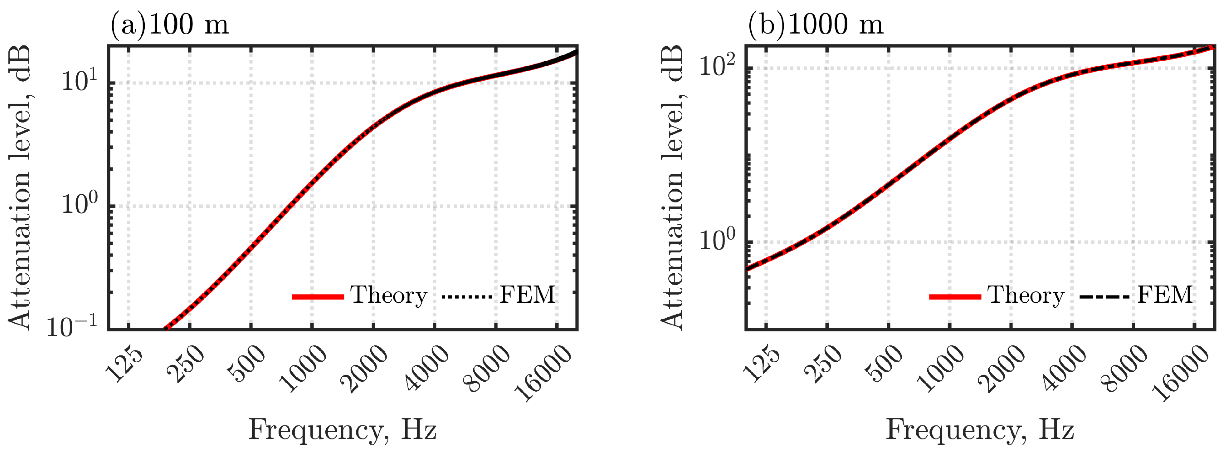
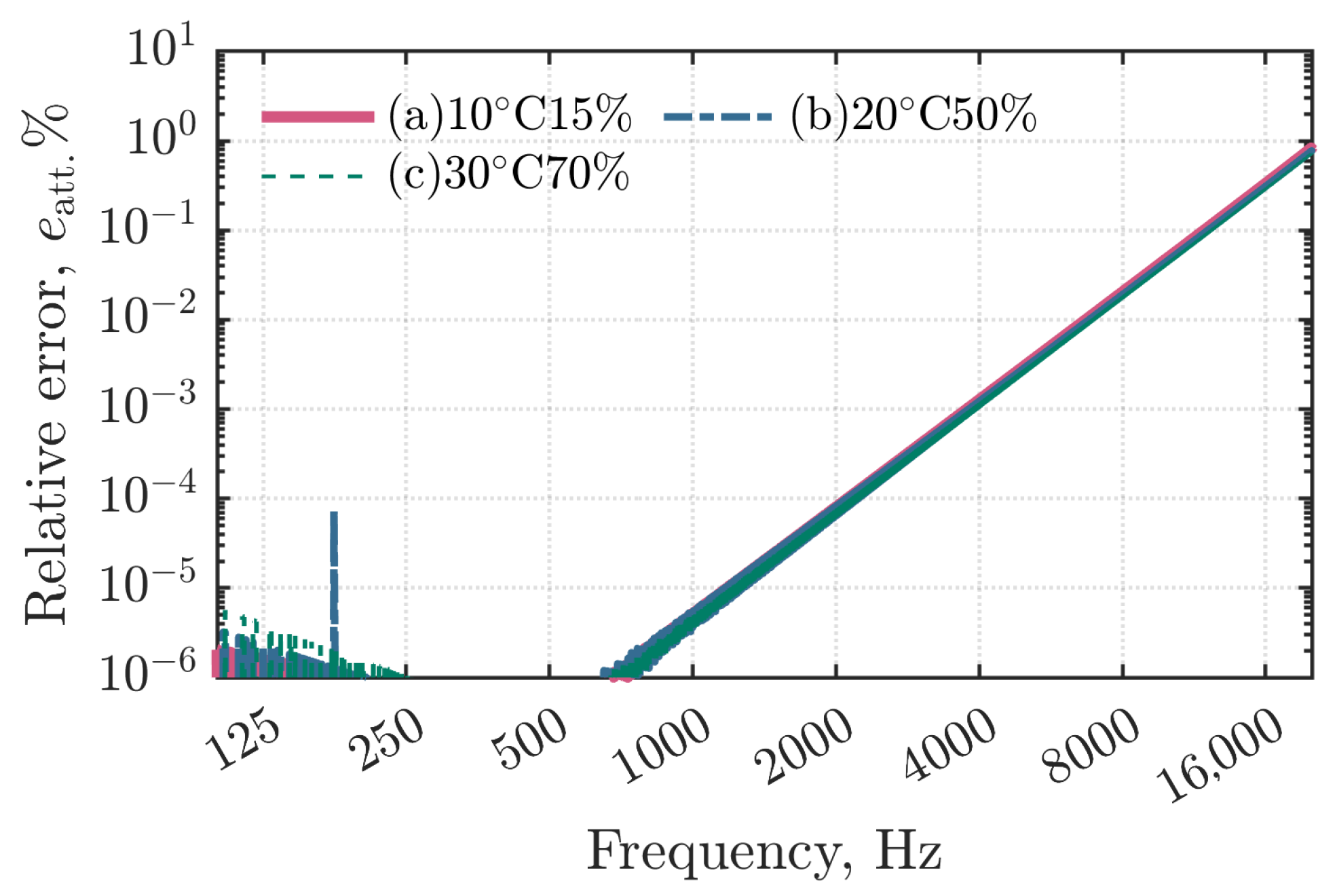
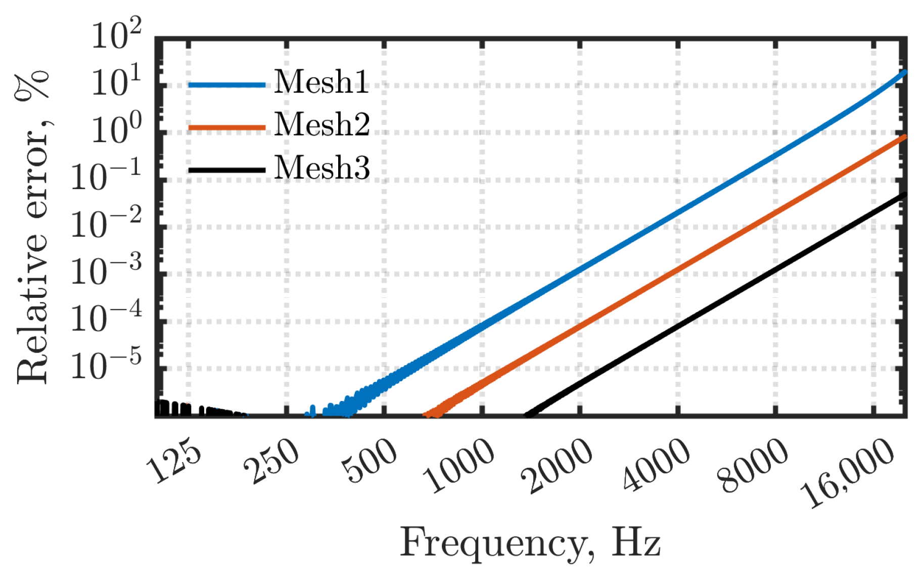
3.2. Results and Discussion

To facilitate intuitive understanding in the agreement between the theory and FEM, Figure 3a,b presents the attenuation levels, $L_{\mathrm{att}.}^{theory}$ and $L_{\mathrm{att}.}^{fem}$, at two receivers x = 100 m and 1000 m, computed using the ISO 9613-1 model (theory) and the lossy Helmholtz equation approach (FEM) for condition (a). Apparently, $L_{\mathrm{att}.}^{fem}$ agrees well with $L_{\mathrm{att}.}^{theory}$ at the two receivers and at frequencies up to 20 kHz. The result is also true for other receivers and conditions (b) and (c). Regarding the error level associated with the lossy Helmholtz equation approach, Figure 4 shows $e_{\mathrm{att}.}$ at the most distant receiver $\mathit{r}=(1000,0)$ for atmospheric conditions (a)–(c). The relative errors become larger for higher frequencies. The error magnitudes are almost equal, irrespective of the atmospheric conditions. For conditions (a)–(c), the maximum values of the relative errors caused at 20 kHz are, respectively, 0.84%, 0.77%, and 0.72%. The results demonstrated that the FEM based on the lossy Helmholtz equation approach can include the air absorption effect accurately at audible frequencies up to 20 kHz using the pure-tone sound attenuation coefficient described in the ISO 9613-1 model.

The error increase over frequencies is attributable to the dispersion error—an inherent error deriving from spatial discretization of the space with FEM. The dispersion error becomes large at higher frequencies for a given FE mesh. A simple strategy to reduce the dispersion error is to use a mesh with higher spatial resolution. Here, we show further how the error magnitude increases or decreases using a mesh with a coarser or higher spatial resolution. Figure 5 shows the $e_{\mathrm{att}.}$ at the most distant receiver $\mathit{r}=(1000,0)$ for the atmospheric conditions (a) when using FE meshes with a spatial resolution of 3.4 (Mesh1) and 13.6 (Mesh3) elements per wavelength at 20 kHz. The two FE meshes have a half spatial resolution of 400,002 DOF and a two times higher spatial resolution of 2,400,003 DOF. In the figure, Mesh2 represents the baseline mesh with a spatial resolution of 6.8 elements per wavelength. Since the used FEM has fourth-order accuracy, the relative errors of Mesh1 increase to about one-sixteenth compared to those of the baseline Mesh2. The error magnitude exceeds 2% at frequencies above about 12 kHz. However, it is important that the error magnitude becomes less than 0.84% at frequencies below 10 kHz, where the spatial resolution of 6.8 elements per wavelength is satisfied. On the other hand, the relative errors of Mesh3 decrease to about one-sixteenth compared to those of Mesh2. The maximum error at 20 kHz is 0.05% for the two-times-higher resolution mesh. Note that we limit our discussion to the idealized case with a mesh discretized by rectangular elements. However, the proposed problem is also helpful in estimating the error characteristics for finite elements with different shape functions and a mesh discretized with irregularly shaped elements.

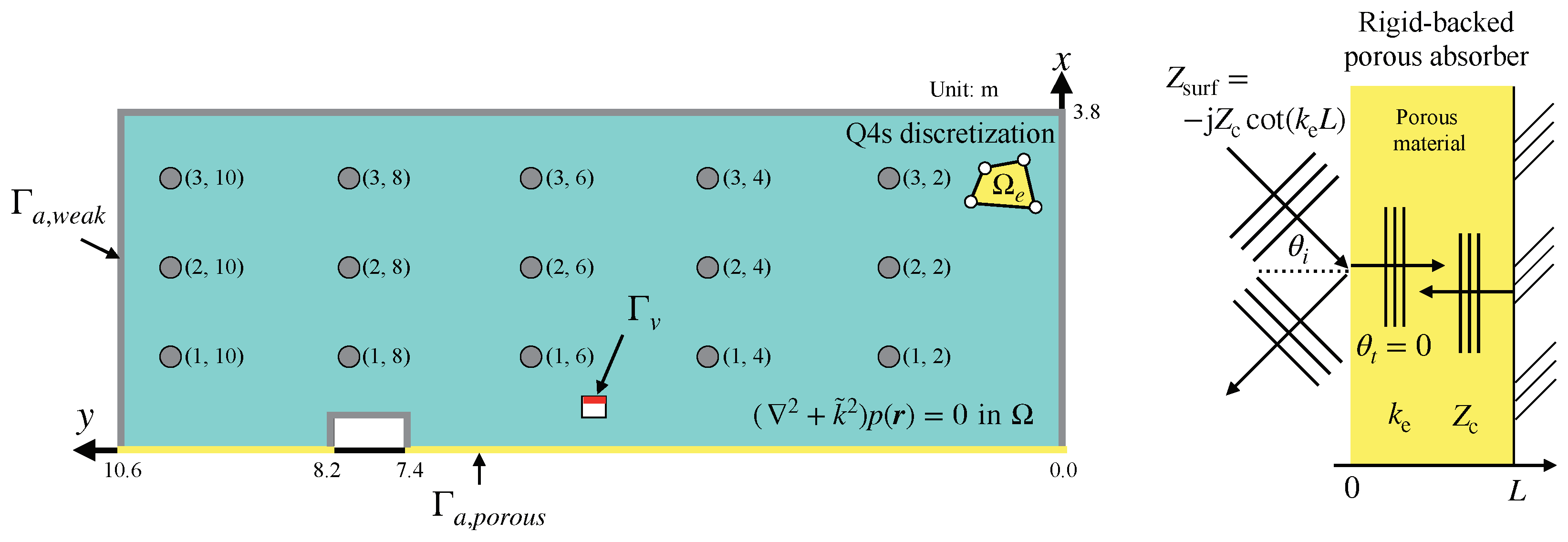
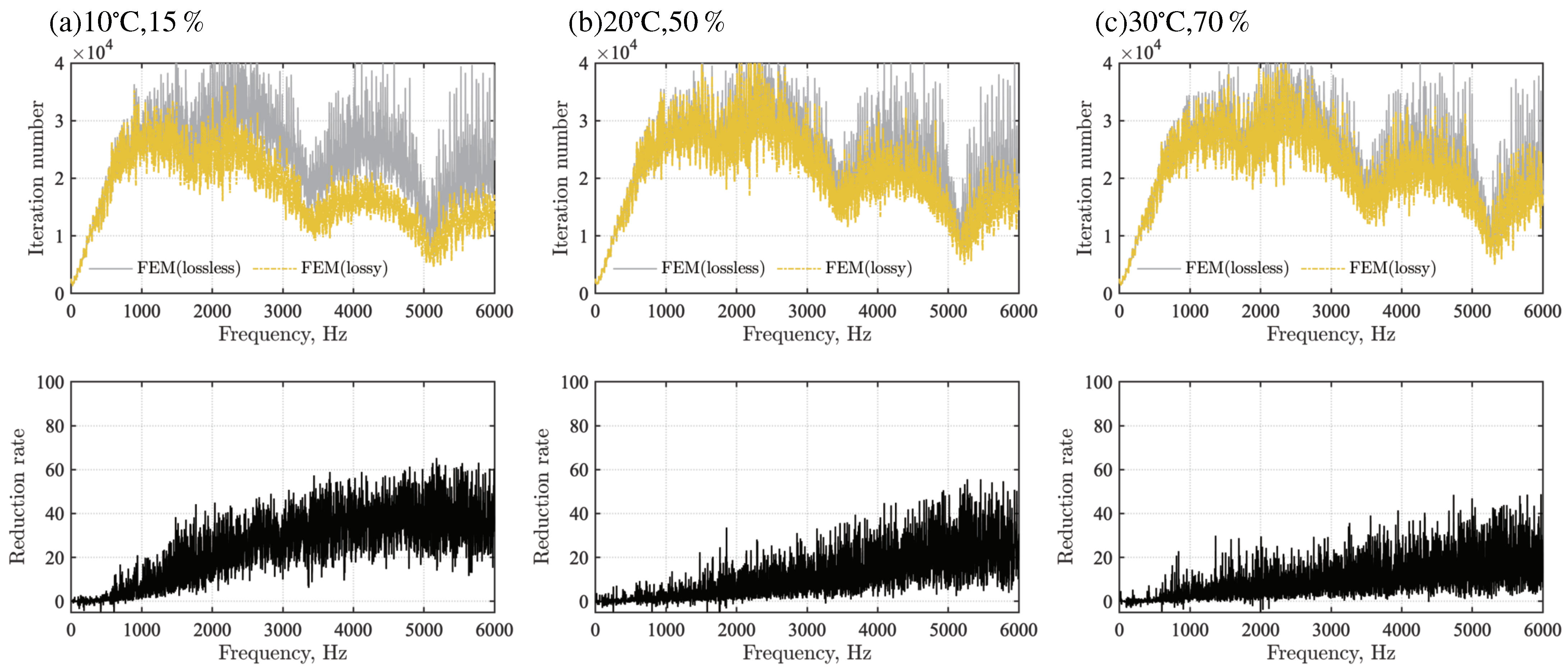
4. Computational Efficiency Assessment with a 2D Office Problem

4.1. Outline of the Problem

This section presents an evaluation of the computational efficiency of 2D room acoustics simulation using the lossy Helmholtz equation-based FEM when using the iterative solver as a linear system solution via a real-scale 2D office problem. The computational efficiency was evaluated by a comparison with the standard lossless Helmholtz equation approach. We also present how room frequency responses change with the air absorption effect. Iterative solvers are well known to be efficient linear system solvers for large-scale problems with vast DOF when they converge rapidly with few iteration numbers. However, the convergence characteristics in the frequency-domain room acoustics simulation, which usually solves the lossless Helmholtz equation, become worse at higher frequencies [54,55]. Therefore, obtaining faster convergence of iterative solvers when solving the lossy Helmholtz equation has a marked effect on computational efficiency in a multi-frequency analysis. It is noteworthy that the present 2D office problem has been used to assess the performance of the dispersion-reduced time-domain FEM, including frequency-dependent impedance boundary conditions and a plane-wave-enriched partition of unity FEM in earlier works [56,57].

Figure 6 presents the 2D office problem, including weakly absorbing impedance boundary ${\mathrm{\Gamma }}_{a,weak}$ and a rigid-backed porous sound absorber represented by a frequency-dependent local-reaction impedance boundary ${\mathrm{\Gamma }}_{a,porous}$. ${\mathrm{\Gamma }}_{a,weak}$ has a real-valued specific acoustic impedance corresponding to the normal-incidence sound absorption coefficient ${\alpha }_0$ = 0.1. For ${\mathrm{\Gamma }}_{a,porous}$, three glass wools with different densities of 24 kg/m³ (GW24K), 32 kg/m³ (GW32K), and 96 kg/m³ (GW96K) were assumed with a thickness L of 25 mm. The surface impedance of the glass wool absorbers $Z_{\mathrm{surf}}$ was computed using the transfer matrix method as $Z_{\mathrm{surf}}=-\mathrm{j}{Z}_{\mathrm{c}}cot\left(k_{\mathrm{e}}L\right)$ using the equivalent fluid model. Here, $Z_{\mathrm{c}}$ and $k_{\mathrm{e}}$, respectively, denote the characteristic impedance and the complex wave number of the equivalent fluid. The Miki model [58], which uses flow resistivity $R_{\mathrm{f}}$ as a material property, was used to describe the fluid properties of the glass wool. The $R_{\mathrm{f}}$ values for GW24K, GW32K, and GW96K are, respectively, 6900 Pa s/m², 13,900 Pa s/m², and 55,000 Pa s/m². The loudspeaker radiating sound wave is modeled by the vibration boundary ${\mathrm{\Gamma }}_v$ with the vibration acceleration of 1 m³/s². We computed the room’s frequency response from 1 Hz to 6 kHz with 1 Hz intervals. The three atmospheric conditions (a)–(c) used in the preceding section were considered, respectively, for the three sound absorbing conditions with GW24K, GW32K, and GW96K: nine acoustic simulations were performed in all. Spatial discretization was also performed with the dispersion-reduced Q4s with element sizes of 0.01 m × 0.01 m. The resulting mesh has 400,720 DOF with a spatial resolution of 5.7 elements per wavelength. All simulations were conducted using a computer (PRIMERGY CX2550/CX2560 M4; Fujitsu Co. Ltd., TYO, JPN) that has two processors (Xeon Gold 6154 3.0 GHz, 18 core; Intel Corp., Santa Clara, CA, USA). The computational code was compiled using a Fortran compiler included in the Intel oneAPI HPC Toolkit (Ver. 2021; Intel Corp.). Parallel computation using OpenMP was conducted with 24 threads.

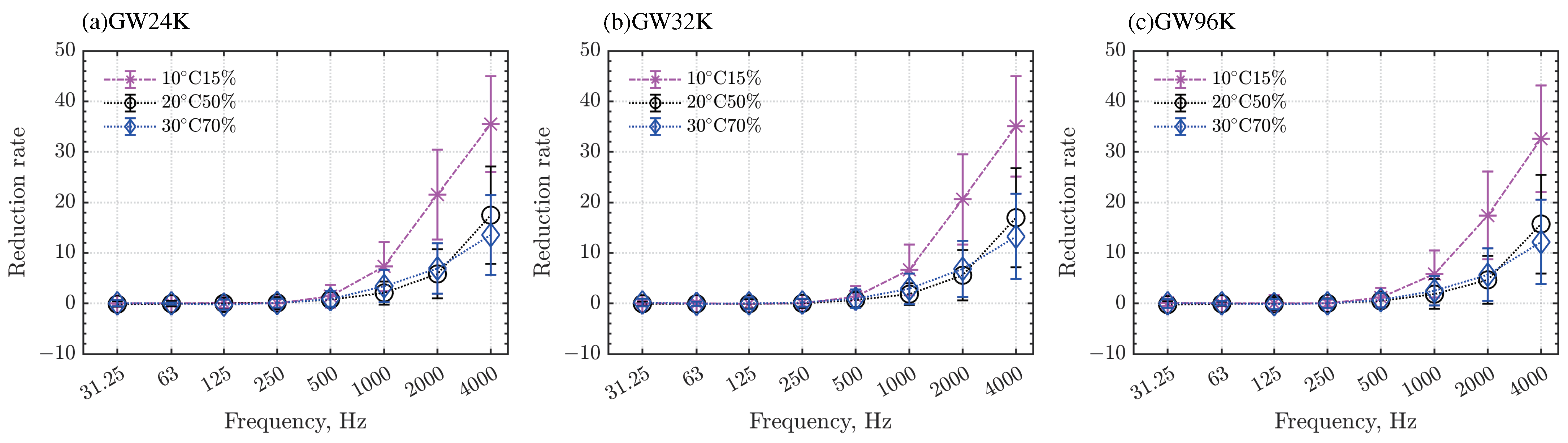
4.2. Results and Discussion

First, as an example to demonstrate how a room’s frequency response changes with the consideration of the air absorption effect, Figure 7 presents a comparison of frequency responses computed using FEMs based on the lossy and lossless Helmholtz equation approaches for the case with the atmospheric condition (a) and with GW24K. Condition (a) is the highest air absorption case, as shown in Figure 2. It can be found that SPL reduction because of the air absorption is especially pronounced at higher frequencies, as expected. Additionally, the air absorption does not influence SPL at frequencies lower than 2 kHz. The magnitude of the pure-tone sound attenuation coefficient is 0.044–0.1 [dB/m] at 2 kHz–6 kHz. Although the GW24K sound absorber has ${\alpha }_0$ > 0.6 at frequencies higher than 2 kHz, consideration of the air absorption still leads to SPL reduction in this case. To measure the degree of the SPL reduction by considering the air absorption, we define the following mean SPL difference D in a 1/3 octave band level over 15 sound receivers, calculated using the FEMs based on the lossy and lossless Helmholtz equations as

$$D=\frac{1}{n_r}\sum _{i=1}^{n_r}[{\overline{L}}_{\mathrm{lossless}}({\mathit{r}}_i,{\omega }_c)-{\overline{L}}_{\mathrm{loss}}({\mathit{r}}_i,{\omega }_c)]\left[\mathrm{dB}\right],$$

(12)

where ${\overline{L}}_{\mathrm{lossless}}({\mathit{r}}_i,{\omega }_c)$ and ${\overline{L}}_{\mathrm{loss}}({\mathit{r}}_i,{\omega }_c)$ represent the $1/3$ octave band SPL at receiver ${\mathit{r}}_i$ and at the center frequency ${\omega }_c$ computed, respectively, by the FEMs based on the lossless and lossy Helmholtz equations. The $n_r(=15)$ is the number of sound receivers. The positive value in D expresses the magnitude of SPL reduction by the air absorption. Figure 8 presents the mean SPL difference D at the three atmospheric conditions (a)–(c) for cases with GW24K, GW32K, and GW96K sound absorbers. Results showed that the order of SPL reduction is consistent with the order of air absorption magnitude, as shown in Figure 2. For the atmospheric conditions (b) and (c), the air absorption effect shows a small impact on the 1/3 octave band SPL with D < 0.5 dB for all frequency bands up to 5 kHz. For the atmospheric condition (a), the air absorption effect is also small, with D < 0.6 dB at frequencies below 2 kHz. We can find an SPL reduction with D values of around 1.0 dB at 4 and 5 kHz. This order of the mean SPL difference may lead to uncertainty in room acoustics prediction, considering the standard deviation of 0.26∼0.36 dB.

The computational efficiency of the FEMs based on the lossy and lossless Helmholtz equations is evaluated by comparing the iteration numbers of both approaches. Results demonstrate that including the air absorption effect has an additional benefit on the computational efficiency at high frequencies. In this evaluation, a smaller iteration number represents higher computational speed. As a quantitative measure, we define the reduction rate $R_{\mathrm{iter}}$ of the iteration numbers as

$$R_{\mathrm{iter}}\left(\omega \right)=\frac{n_{\mathrm{lossless}}\left(\omega \right)-n_{\mathrm{loss}}\left(\omega \right)}{n_{\mathrm{lossless}}\left(\omega \right)}\times 100[\%],$$

(13)

where $n_{\mathrm{lossless}}\left(\omega \right)$ and $n_{\mathrm{loss}}\left(\omega \right)$, respectively, denote iteration numbers of the CSQMOR method at frequency $\omega$. It is noteworthy that we used the iteration number required for convergence as a measure to evaluate the computational efficiency because the iteration process of iterative solvers is the most time-consuming part of FEM in the frequency domain. In the presented simulation cases, the process consumes more than 95% of the computational time.

Figure 9a,c presents the results of the iteration number comparison in both approaches for the cases with three atmospheric conditions (a)–(c) and with the GW24K absorber. The lower part of the figure shows the reduction rate of the iteration number $R_{\mathrm{iter}}$. Overall, it is apparent that there are fewer iteration numbers in the lossy Helmholtz equation approach at a higher frequency range for the three atmospheric conditions. We can find that the reduction rate differs for three atmospheric conditions. The atmospheric condition (a) has the highest iteration number reduction. The reduction rate reaches approximately 60% for high frequencies. In addition, higher reduction can be found at lower frequencies than in either condition (b) or (c). In fact, condition (c) shows the lowest iteration number reduction, but the reduction rate reaches 40% at high frequencies.

To explain further how atmospheric conditions influence the reduction rate, Figure 10a and Figure 10c, respectively, show a 1/3 octave band averaged reduction rate at three atmospheric conditions for cases with GW24K, GW32K, and GW96K sound absorbers. In the figure, the error bar represents the standard deviation values. The reduction rates are related clearly to the magnitude of the pure-tone sound attenuation coefficient for frequencies higher than 1 kHz. For frequencies of 1 kHz–2 kHz, the values of pure-tone sound attenuation coefficients are larger in the order of atmospheric conditions (a), (c), and (b) as in Figure 2. This order corresponds to the reduction rate in the iteration number as in Figure 10a,c: higher air absorption engenders fewer iteration quantities of the iterative solver. At 4 kHz, the order in the magnitude of the air absorption changes for conditions (b) and (c), at which the atmospheric condition (b) has larger pure-tone sound attenuation coefficients than those in condition (c). As in Figure 10a,c, the reduction rates in the iteration number are larger for condition (b) than for condition (c). Apparently, the value of the pure-tone sound attenuation coefficient larger than 0.03 has a notable effect on the convergence speed of the iterative solver. In the presented cases, the averaged reduction rate at the 4 kHz band shows a 33–36% computational time reduction for atmospheric condition (a). The computational time reductions for atmospheric conditions (b) and (c), respectively, reached 16–17% and 12–14%.

As a reference, Figure 11 presents the convergence history of the iterative solver in FEMs based on the lossy and lossless Helmholtz equations at 4704 Hz for the atmospheric conditions (a) with the GW32K absorber. At the frequency, the maximum reduction rate of 66% is achieved. The convergence speed changed around at the value of the relative residual 2-norm of 10${}^{-3}$. The lossy Helmholtz equation-based FEM shows faster decreases in the residual norm.

Finally, we further show whether or not the faster convergence holds when using a higher spatial resolution mesh for the atmospheric conditions (a) with the GW24K absorber. We tested the convergence property of the iterative solver at four pure tones, 3 kHz, 4 kHz, 5kHz, and 6 kHz, for a mesh with an element size of 0.005 m × 0.005 m, having a spatial resolution of 11.5 elements per wavelength. The resulting mesh has 1,599,840 DOF.

Table 1. Iteration number and CPU time $t_{\mathrm{cpu}}$ for FEMs based on the lossy and lossless Helmholtz equations: reduction rate of the iteration number $R_{\mathrm{iter}}$ and CPU time $R_{\mathrm{cpu}}$ are also shown in parentheses.

	FEM (Lossless)		FEM (Lossy)
Frequency, Hz	${\mathit{n}}_{\mathrm{lossless}}$	${\mathit{t}}_{\mathrm{cpu}}$, s	${\mathit{n}}_{\mathrm{loss}}$(${\mathit{R}}_{\mathrm{iter}}$, %)	${\mathit{t}}_{\mathrm{cpu}}$, s (${\mathit{R}}_{\mathrm{cpu}}$, %)
3000	40,561	200	29,334 (27.7)	145 (27.5)
4000	36,883	183	24,615 (33.3)	123 (32.7)
5000	24,477	121	16,567 (32.3)	83 (31.1)
6000	37,811	187	23,132 (38.8)	114 (39.2)

lists the iteration number and CPU time $t_{\mathrm{cpu}}$ for FEMs based on the lossy and lossless Helmholtz equations. The reduction rates of iteration number and CPU time are also shown as $R_{\mathrm{iter}}$ and $R_{\mathrm{cpu}}$. Results showed fewer iteration numbers for the FEM based on the lossy Helmholtz equation. Therefore, faster convergence still holds for the higher spatial resolution mesh. The iteration number and CPU time reductions, respectively, reached 27.7–38.8% and 27.5–39.2%. To show how efficiency changes with different spatial resolution meshes,

Table 2. Ratio of the iteration number over DOF and iteration number increase rate for meshes with a different spatial resolution.

	${\mathit{n}}_{\mathbf{loss}}/\mathbf{DOF}\times 100\%$
Frequency, Hz	Mesh1	Mesh2	${\mathit{n}}_{\mathrm{loss}}^{\mathrm{Mesh}2}/{\mathit{n}}_{\mathrm{loss}}^{\mathrm{Mesh}1}$
3000	19.1	1.8	1.5
4000	15.2	1.5	1.6
5000	9.3	1.0	1.8
6000	14.4	1.4	1.6

presents the ratio of iteration number over DOF denoted as $n_{\mathrm{loss}}/\mathrm{DOF}\times 100[\%]$ and the iteration number increase rate denoted as $n_{\mathrm{loss}}^{\mathrm{Mesh}2}/n_{\mathrm{loss}}^{\mathrm{Mesh}1}$ for the four frequencies. Here, Mesh1 and Mesh2 represent, respectively, the baseline mesh with 400,720 DOF and the two-times-higher resolution mesh with 1,599,840 DOF. Additionally, $n_{\mathrm{loss}}^{\mathrm{Mesh}1}$ and $n_{\mathrm{loss}}^{\mathrm{Mesh}2}$, respectively, present $n_{\mathrm{loss}}\mathrm{s}$ for Mesh1 and Mesh2. It can be found that Mesh2 with a higher spatial resolution shows fewer iteration numbers over DOF at the four frequencies. The $n_{\mathrm{loss}}\mathrm{s}$ are only 1.0–1.8% against the DOF, which is about 1/10 of Mesh1. The iteration number increase rate at the four frequencies is frequency-independent and shows an almost constant value of 1.5–1.8. This indicates that the convergence trend of the lossy Helmholtz equation-based FEM does not change even with the use of a higher resolution mesh, but the iteration number increase is smaller than the increase of DOF. As a reference, the memory requirement of FEMs based on the lossy and lossless Helmholtz equations are the same. They are 151 MByte and 600 MByte for Mesh1 and Mesh2, respectively. Therefore, the lossy Helmholtz equation-based FEM does not require additional computational cost to include the air absorption effect.

5. Conclusions

This paper presents the accuracy and computational efficiency assessment results of a frequency-domain FEM based on the lossy Helmholtz equation approach, which can incorporate air absorption effects using the pure-tone sound attenuation coefficient according to the ISO 9613-1 model. In the approach, air absorption is added as volume absorption to the spaces. Two numerical problems were used for the assessment. The plane-wave propagation problem in a long duct with a length of 1 km revealed that the lossy Helmholtz equation based FEM can include a sound attenuation effect accurately up to 20 kHz with relative error below 1% from theoretical attenuation levels when using FE meshes having spatial resolution of about seven elements per wavelength. As a fundamental error characteristic, the error in the attenuation levels increases linearly over frequencies in both logarithmic axis graphs. The error level can be reduced using a mesh with higher spatial resolution. Then, the sound propagation problem in a real-scale office revealed that the lossy Helmholtz equation based FEM is more computationally efficient than the lossless one at higher frequencies when using CSQMOR iterative solver as a linear system equation solver at each frequency. The increased effect of computational efficiency is related strongly with the magnitude of the pure-tone sound attenuation coefficient. The atmospheric condition with a larger air absorption effect, having a larger pure-tone sound attenuation coefficient value, engenders higher computational efficiency with fewer iteration numbers. From these results, we can infer that the lossy Helmholtz equation-based FEM might be helpful when one simulates room acoustics at high frequencies of the computational efficiency aspect. However, our discussion is limited to 2D cases. Therefore, further examination of three-dimensional room acoustics simulation is crucially important. Although we did not examine lossy Helmholtz equation-based discretization, it might be beneficial for other numerical methods, such as a high-order FEM and BEM with iterative solvers. For example, a recent work [59] focused on solving car interior acoustics up to 20 kHz with the partition of unity isogeometric analysis.

Finally, as mentioned in the present paper’s introduction, the following three essential research directions currently exist in room acoustics simulation, each with a different attractive capability and applicability.

• The use of geometrical acoustics simulation methods and presenting methods to improve accuracy, such as phase beam tracing and the novel scattering algorithm [60].
• The use of wave-based acoustics simulation methods and presenting methods to improve their efficiency.
• The use of hybrid techniques that combine geometrical acoustics simulation and wave-based acoustics simulation methods.

With the continuous research in the above directions, computational room acoustics simulation methods will be a further effective tool in a broad range of applications.

References

1. Savioja, L.; Xiang, N. Simulation-based auralization of room acoustics. Acoust. Today 2020, 16, 48–56. [Google Scholar] [CrossRef]
2. Vorländer, M. Are virtual sounds real? Acoust. Today 2020, 16, 46–54. [Google Scholar] [CrossRef]
3. Savioja, L.; Svensson, U.P. Overview of geometrical room acoustic modeling techniques. J. Acoust. Soc. Am. 2015, 138, 708–730. [Google Scholar] [CrossRef]
4. Krokstad, A.; Strøm, S.; Sørsdal, S. Calculating the acoustical room response by the use of a ray tracing technique. J. Sound Vib. 1968, 8, 118–125. [Google Scholar] [CrossRef]
5. Allen, J.B.; Berkley, D.A. Image method for efficiently simulating small-room acoustics. J. Acoust. Soc. Am. 1979, 65, 943–950. [Google Scholar] [CrossRef]
6. Hodgson, M.; Wareing, A. Comparisons of predicted steady-state levels in rooms with extended- and local-reaction bounding surfaces. J. Sound Vib. 2008, 309, 167–177. [Google Scholar] [CrossRef]
7. Hodgson, M.; Behrooz, Y. Energy- and wave-based beam-tracing prediction of room-acoustical parameters using different boundary conditions. J. Acoust. Soc. Am. 2012, 132, 1450–1461. [Google Scholar]
8. Jeong, C.H. Absorption and impedance boundary conditions for phased geometrical-acoustics methods. J. Acoust. Soc. Am. 2012, 132, 2347–2358. [Google Scholar] [CrossRef]
9. Jeong, C.H.; Ih, J.G.; Rindel, J.H. An approximate treatment of reflection coefficient in the phased beam tracing method for the simulation of enclosed sound fields at medium frequencies. Appl. Acoust. 2008, 69, 601–613. [Google Scholar] [CrossRef]
10. Sakamoto, S. Phase-error analysis of high-order finite difference time domain scheme and its influence on calculation results of impulse response in closed sound field. Acoust. Sci. Tech. 2007, 28, 295–309. [Google Scholar] [CrossRef]
11. Sakamoto, S.; Nagatomo, H.; Ushiyama, A.; Tachibana, H. Calculation of impulse responses and acoustic parameters in a hall by the finite-difference time-domain method. Acoust. Sci. Tech. 2008, 29, 256–265. [Google Scholar] [CrossRef]
12. Kowalczyk, K.; van Walstijn, M. Room acoustics simulation using 3-D compact explicit FDTD schemes. IEEE Trans. Audio Speech Lang. Process. 2011, 19, 34–46. [Google Scholar] [CrossRef]
13. Hamilton, B.; Bilbao, S. FDTD methods for 3-D room acoustics simulation with high-order accuracy in space and time. IEEE/ACM Trans. Audio Speech Lang. Process. 2017, 25, 2112–2124. [Google Scholar] [CrossRef]
14. Cingolani, M.; Fratoni, G.; Barbaresi, L.; D’Orazio, D.; Hamilton, B.; Garai, M. A trial acoustic improvement in a lecture hall with MPP sound absorbers and FDTD acoustic simulations. Appl. Sci. 2021, 11, 2445. [Google Scholar] [CrossRef]
15. Murillo, D.M.; Fazi, F.M.; Astley, J. Room acoustic simulations using the finite element method and diffuse absorption coefficients. Acta Acust. United Acust. 2019, 105, 231–239. [Google Scholar] [CrossRef]
16. Pind, F.; Engsig-Karup, A.P.; Jeong, C.-H.; Hesthaven, J.S.; Mejling, M.S.; Strømann-Andersen, J. Time domain room acoustic simulations using the spectral element method. J. Acoust. Soc. Am. 2019, 145, 3299–3310. [Google Scholar] [CrossRef]
17. Prinn, A.G. A review of finite element methods for room acoustics. Acoustics 2023, 5, 367–395. [Google Scholar] [CrossRef]
18. Yoshida, T.; Okuzono, T.; Sakagami, K. A parallel dissipation-free and dispersion-optimized explicit time-domain FEM for large-scale room acoustics simulation. Buildings 2022, 12, 105. [Google Scholar] [CrossRef]
19. Yoshida, T.; Okuzono, T.; Sakagami, K. Binaural auralization of room acoustics with a highly scalable wave-based acoustics simulation. Appl. Sci. 2023, 13, 2832. [Google Scholar] [CrossRef]
20. Okuzono, T.; Yoshida, T. High potential of small-room acoustic modeling with 3D time-domain finite element method. Front. Built Environ. 2022, 8, 1006365. [Google Scholar] [CrossRef]
21. Hargreaves, J.A.; Cox, T.J. A transient boundary element method model of Schroeder diffuser scattering using well mouth impedance. J. Acoust. Soc. Am. 2008, 124, 2942–2951. [Google Scholar] [CrossRef]
22. Yasuda, Y.; Ueno, S.; Kadota, M.; Sekine, H. Applicability of locally reacting boundary conditions to porous material layer backed by rigid wall: Wave-based numerical study in non-diffuse sound field with unevenly distributed sound absorbing surfaces. Appl. Acoust. 2016, 113, 45–57. [Google Scholar] [CrossRef]
23. Yasuda, Y.; Saito, K.; Sekine, H. Effects of the convergence tolerance of iterative methods used in the boundary element method on the calculation results of sound fields in rooms. Appl. Acoust. 2020, 157, 106997. [Google Scholar] [CrossRef]
24. Gumerov, N.A.; Duraiswami, R. Fast multipole accelerated boundary element methods for room acoustics. J. Acoust. Soc. Am. 2021, 150, 1707–1720. [Google Scholar] [CrossRef]
25. Cardoso Soares, M.; Brandão Carneiro, E.; Aizik Tenenbaum, R.; Mareze, P.H. Low-frequency room acoustical simulation of a small room with BEM and complex-valued surface impedances. Appl. Acoust. 2022, 188, 108570. [Google Scholar] [CrossRef]
26. Aretz, M.; Vorländer, M. Combined wave and ray based room acoustic simulations of audio systems in car passenger compartments, Part I: Boundary and source data. Appl. Acoust. 2014, 76, 82–99. [Google Scholar] [CrossRef]
27. Aretz, M.; Vorländer, M. Combined wave and ray based room acoustic simulations of audio systems in car passenger compartments, Part II: Comparison of simulations and measurements. Appl. Acoust. 2014, 76, 52–65. [Google Scholar] [CrossRef]
28. Cox, T.J.; Peter, D. Porous sound absorption. In Acoustic Absorbers and Diffusers: Theory, Design and Application; Taylor & Francis: London, UK, 2017; pp. 175–224. [Google Scholar]
29. Cox, T.J.; Peter, D. Resonant absorbers. In Acoustic Absorbers and Diffusers: Theory, Design and Application; Taylor & Francis: London, UK, 2017; pp. 225–264. [Google Scholar]
30. ISO 10534-2:1998; Acoustics—Determination of Sound absorption Coefficient and Impedance in Impedance Tubes—Part 2: Transfer-Function Method. International Organization for Standardization: Geneva, Switzerland, 1998.
31. Brandão, E.; Lenzi, A.; Paul, S. A review of the In Situ impedance and sound absorption measurement techniques. Acta Acust. United Acust. 2015, 101, 443–463. [Google Scholar] [CrossRef]
32. Allard, J.; Atalla, N. Modeling multilayered systems with porous materials using the transfer matrix method. In Propagation of Sound in Porous Media: Modeling Sound Absorbing Materials; John Wiley & Sons: Chichester, UK, 2009; pp. 243–281. [Google Scholar]
33. Craggs, A. A finite element model for rigid porous absorbing materials. J. Sound Vib. 1978, 61, 101–111. [Google Scholar] [CrossRef]
34. Craggs, A. Coupling of finite element acoustic absorption models. J. Sound Vib. 1979, 66, 605–613. [Google Scholar] [CrossRef]
35. Allard, J.; Atalla, N. Finite element modelling of poroelastic materials. In Propagation of Sound in Porous Media: Modeling Sound Absorbing Materials; John Wiley & Sons: Chichester, UK, 2009; pp. 309–349. [Google Scholar]
36. Kates, J.M.; Brandewie, E.J. Adding air absorption to simulated room acoustic models. J. Acoust. Soc. Am. 2020, 148, EL408–EL413. [Google Scholar] [CrossRef]
37. ISO 9613-1:1993; Acoustics—Attenuation of Sound during Propagation Outdoors. Part 1: Calculation of the Absorption of Sound by the Atmosphere. International Organization for Standardization: Geneva, Switzerland, 1993.
38. Saarelma, J.; Savioja, L. Audibility of dispersion error in room acoustic finite-difference time-domain simulation in the presence of absorption of air. J. Acoust. Soc. Am. 2016, 140, EL545–EL550. [Google Scholar] [CrossRef]
39. Hamilton, B. Air absorption filtering method based on approximate green function for Stokes equation. In Proceedings of the 24th International Conference on Digital Audio Effects, Vienna, Austria, 8–10 September 2021; pp. 160–167. [Google Scholar]
40. Hamilton, B.; Bilbao, S. Time-domain modeling of wave-based room acoustics including viscothermal and relaxation effects in air. JASA Express Lett. 2021, 1, 092401-1–092401-8. [Google Scholar] [CrossRef]
41. Ihlenburg, F. Sound in vibrating cabins: Physical effects, mathematical formulation, computational simulation with FEM. In Computational Aspects of Structural Acoustics and Vibration; Sandberg, G., Ohayon, R., Eds.; Springer: Wien, Austria, 2008; pp. 103–170. [Google Scholar]
42. Sakuma, T.; Iwase, T.; Yasuoka, M. Prediction of sound fields in rooms with membrane materials: Development of a limp membrane element in acoustical FEM analysis and its application. J. Archit. Plann. Environ. Eng. 1998, 505, 1–8. [Google Scholar]
43. Chen, W.H.; Lee, F.C.; Chiang, D.M. On the acoustic absorption of porous materials with different surface shapes and perforated plates. J. Sound Vib. 2000, 237, 337–355. [Google Scholar] [CrossRef]
44. Tomiku, R.; Otsuru, T. Sound fields analysis in an irregular-shaped reverberation room by finite element method. J. Archit. Plann. Environ. Eng. 2002, 551, 9–15. [Google Scholar] [CrossRef]
45. Aretz, M.; Vorländer, M. Efficient modeling of absorbing boundaries in room acoustic FE simulations. Acta Acust. United Acust. 2010, 96, 1042–1050. [Google Scholar] [CrossRef]
46. Kim, K.H.; Yoon, G.H. Absorption performance optimization of perforated plate using multiple-sized holes and a porous separating partition. Appl. Acoust. 2017, 120, 21–37. [Google Scholar] [CrossRef]
47. Okuzono, T.; Sakagami, K. Dispersion error reduction of absorption finite elements based on equivalent fluid model. Acoust. Sci. Tech. 2018, 39, 362–365. [Google Scholar] [CrossRef]
48. Carbajo, J.; Ramis, J.; Godinho, L.; Mendes, P.A. Assessment of methods to study the acoustic properties of heterogeneous perforated panel absorbers. Appl. Acoust. 2018, 133, 1–7. [Google Scholar] [CrossRef]
49. Okuzono, T.; Nitta, T.; Sakagami, K. Note on microperforated panel model using equivalent-fluid-based absorption elements. Acoust. Sci. Tech. 2019, 40, 221–224. [Google Scholar] [CrossRef]
50. Davis, T.A. Direct Methods for Sparse Linear Systems; SIAM: Philadelphia, PA, USA, 2006. [Google Scholar]
51. Barrett, R.; Berry, M.; Chan, T.; Demmel, J.; Donato, J.; Dongarra, J.; Eijkhout, V.; Pozp, R.; Romine, C.; van der Vorst, H. Nonstationary iterative methods. In Templates for the Solution of Linear Systems: Building Blocks for Iterative Methods; SIAM: Philadelphia, PA, USA, 1994; pp. 14–20. [Google Scholar]
52. Zhang, J.; Dai, H. A new quasi-minimal residual method based on a biconjugate A-orthonormalization procedure and coupled two-term recurrences. Numer. Algorithms 2015, 70, 875–896. [Google Scholar] [CrossRef]
53. Guddati, M.N.; Yue, B. A Modified integration rules for reducing dispersion error in finite element methods. Comput. Methods Appl. Mech. Engrg. 2004, 193, 275–287. [Google Scholar] [CrossRef]
54. Okamoto, N.; Tomiku, R.; Otsuru, T.; Yasuda, Y. Numerical analysis of large-scale sound fields using iterative methods part II: Application of Krylov subspace methods to finite element analysis. J. Comput. Acoust. 2007, 15, 473–493. [Google Scholar] [CrossRef]
55. Okuzono, T.; Sakagami, K. A frequency domain finite element solver for acoustic simulations of 3D rooms with microperforated panel absorbers. Appl. Acoust. 2018, 129, 1–12. [Google Scholar] [CrossRef]
56. Okuzono, T.; Mohamed, M.S.; Sakagami, K. Potential of room acoustic solver with plane-wave enriched finite element method. Appl. Sci. 2020, 10, 1969. [Google Scholar] [CrossRef]
57. Okuzono, T.; Yoshida, T.; Sakagami, K. Efficiency of room acoustic simulations with time-domain FEM including frequency-dependent absorbing boundary conditions: Comparison with frequency-domain FEM. Appl. Acoust. 2021, 182, 108212. [Google Scholar] [CrossRef]
58. Miki, Y. Acoustical properties of porous materials – Modifications of Delany–Bazley models. J. Acoust. Soc. Jpn. 1990, 11, 19–24. [Google Scholar] [CrossRef]
59. Diwan, G.C.; Mohamed, M.S. Pollution studies for high order isogeometric analysis and finite element for acoustic problems. Comput. Methods Appl. Mech. Eng. 2019, 350, 701–718. [Google Scholar] [CrossRef]
60. Autio, H.; Nilsson, E. A novel algorithm for directional scattering in acoustic ray tracers. Acoustics 2023, 5, 928–947. [Google Scholar] [CrossRef]
Figure 1. Plane wave propagation problem in 2D long duct.
Applsci 14 00194 g001
Figure 2. Pure-tone sound attenuation coefficient for three atmospheric conditions (a)–(c).
Applsci 14 00194 g002
Figure 3. Attenuation levels at two receivers for atmospheric conditions (a) computed using the ISO 9613-1 model (theory) and the Helmholtz equation approach (FEM): (a) x = 100 m, and (b) x = 1000 m.
Applsci 14 00194 g003
Figure 4. Relative errors in attenuation levels for three atmospheric conditions (a)–(c) when using the FE mesh with a spatial resolution of 6.8 elements per wavelength.
Applsci 14 00194 g004
Figure 5. Relative errors in attenuation levels for atmospheric condition (a) when using Mesh1–3, respectively, with a spatial resolution of 3.4, 6.8, and 13.6 elements per wavelength.
Applsci 14 00194 g005
Figure 6. Sound propagation problem in a 2D office. A total of 15 sound receivers represented by gray circles are placed inside the room. The rigid-backed porous sound absorber is modeled with surface impedance Z surf as a local-reaction material in which a plane wave with incidence angle θ i propagates inside materials as the transmission angle θ t = 0 .
Applsci 14 00194 g006
Figure 7. Comparison of room frequency responses at r = ( 1 , 2 ) computed using FEMs based on the lossy and lossless Helmholtz equation approaches for the case with atmospheric condition (a) and with GW24K: (upper) frequency response at 1 Hz to 3000 Hz and (lower) frequency response at 3 kHz–6 kHz.
Applsci 14 00194 g007
Figure 8. Comparison of mean SPL reduction D at three atmospheric conditions for cases with (a) GW24K, (b) GW32K, and (c) GW96K.
Applsci 14 00194 g008
Figure 9. Comparison of iteration numbers in FEMs based on the lossy and lossless Helmholtz equation approaches for cases with the GW24K sound absorber: (left) atmospheric condition (a), (center) atmospheric condition (b), (right) atmospheric condition (c). Lower figures show the reduction rate R iter .
Applsci 14 00194 g009
Figure 10. Comparison of the 1/3 octave band averaged reduction rate on the FEM based on the lossy Helmholtz equation approach at three atmospheric conditions for cases with (a) GW24K, (b) GW32K, and (c) GW96K sound absorbers. The error bars represents the standard deviation values.
Applsci 14 00194 g010
Figure 11. Comparison of convergence history of the iterative solver at 4704 Hz in FEMs based on lossy and lossless Helmholtz equations. Results are shown for atmospheric conditions (a) with the GW32K absorber.
Applsci 14 00194 g011