
Energies of Mechanical Fractional-Order Elements: Causal Concept and Kernel Effects


Department of Chemical Engineering, University of Chemical Technology and Metallurgy, 8 Kliment Ohridsky, blvd., 1756 Sofia, Bulgaria
Appl. Sci. 2024, 14(1), 197; https://doi.org/10.3390/app14010197
Submission received: 6 December 2023
/
Revised: 21 December 2023
/
Accepted: 23 December 2023
/
Published: 25 December 2023
(This article belongs to the Section Mechanical Engineering)
Abstract
:The energies of the classical Maxwell mechanical model of viscoelastic behavior have been studied as a template with a variety of relaxation kernels in light of a causal formulation of the force–displacement relationship. The starting point uses the Lorenzo–Hartley model with the time-fractional Riemann–Liouville derivative. This approach has been reformulated based on critical analysis, allowing for the application of a variety of relaxation (memory) functions mainly based on the Mittag-Leffler family, in order to meet the need for broader modeling of viscoelastic behavior. The examples provided include cases of the types of forces used by Lorenzo and Hartley as well as a new family of force approximations such as a general power-law ramp, polynomials, and the Prony series.
1. Introduction
The energy concept in the fractional models, mainly in mechanics, is an old problem [1,2,3,4,5], based on power-law memory functions, and as such we skip unusual reference quotations (when this is needed in the development of this, study such references will be adequately cited). The main motivation for this study comes from two sources in fractional calculus: first, the work of Lorenzo and Hartley [6]; and second, the experimental and modeling results that go beyond the traditional singular power-law kernel [7] by applying a variety of relaxation functions (memories) in the characterization of viscoelastic materials, mainly based on the family of the Mittag-Leffler function [8,9].
The initial step of this study was inspired by the research of Lorenzo and Hartley [6] on the energies of mechanical fractional elements, where elegant derivations applying the Riemann–Liouville time fractional derivative were developed. However, despite this admiration, the formulation used in the initial study is too narrow, in that the modeling focused on the behavior of viscoelastic material, that is, only cases where the power-law relaxation behavior is observed. Moreover, the force–displacement relationship used in [6] was not causal (see the explanation in the following Section 2). Starting with a new causal formulation in light of the work of Lorenzo and Hartley [6] (see Section 2.4), the research reported here is motivated towards a broader family of relaxation kernels, thereby meeting the problems imposed by the behaviors of real materials [8,9]. This step allows us to see how energies of different viscoelastic relaxations can be modeled (and calculated) and what challenging problems appear beyond the existing Lorenzo–Hartley results. The focus and the main idea of this study are formulated next.
1.1. Aim
The focus of this study is on the energies of mechanical fractional elements in light of memory kernel approximations defined by the properties of the modeled viscoelastic media. The main issue, forming the approach applied here, is the causal formulation of the force–displacement relationship via nonlocal integral relations. The basic Maxwell element (see Figure 1) is used as a template, allowing for easy comparisons with existing literature results.
It is worth noting that the formulations developed in this work only apply causal integral relationships, thereby avoiding conjecture and contradictory interpretations with variants of fractional operators with kernels other than the power law, which is employed by the Riemann–Liouville and Caputo derivatives and has given rise to heated debates in the fractional calculus community (see the commentary in [9]).
1.2. Textual Organization
The remainder of this paper is organized as follows: Section 2 considers the main idea of Lorenzo and Hartley [6] with a critical analysis of the non-causality of their formulation (Section 2.1). A new causal formulation is suggested (Section 2.2), and two examples from [6] are solved in a new manner in Section 2.4. The effect of the initialization, following Lorenzo and Hartley [6], is presented in Section 2.6 with a few critical comments while focusing on its physical relevance. The general principle of causality is presented in Section 3 as concerns its philosophical, physical, and mathematical aspects relating to dynamic systems. The causality principle from the author’s point of view is exemplified in Appendix A.
New examples stepping beyond the results of Lorenzo and Hartley, with the Riemann–Liouville integral as a force-displacement relationship are developed in Section 4 concerning a power-law force ramp (Section 4.1), polynomial force (Section 4.2), exponential force ramp (Section 4.3), and ramp force approximated by Prony’s series (Section 4.4).
More general formulations of the causal force–displacement relationship are developed in Section 5. The approach is exemplified by applications of memory kernels based on single exponential memory (Section 5.1), multi-exponential memory (Prony’s series) (Section 5.1.4), the Mittag-Leffler function (one-parameter) (Section 5.2), and the Prabhakar function (Section 5.3).
All definitions of functions and operators are summarized in Appendix A and Appendix B.
2. Lorenzo–Hartley Concept: A Thorough Evaluation and New Causal Interpretation
Before formulating the main task of this study, we are obliged to demonstrate the background in order to see what is useful and what can be interpreted in the sense of dynamic causality as the main principle of nonlocality, which we do through two examples from the original work [6]. The starting models consider a spring and a dashpot connected in a series (Maxwell model), as explored by Lorenzo and Hartley [6]. We are concerned here with two basic formulations of the force–displacement relationship, and consequently the energy of the fractional elements, which are discussed next.
2.1. Force–Displacement Relationship: Non-Causal Formulation
Following Lorenzo and Hartley [6], the relationship between the force and displacement is presented through the Riemann–Liouville derivative (in original notations):
where
is a time-fractional derivative in the Riemann–Liouville sense [7].
For , we obtain (viscous behavior), while for we have (or more explicitly, Hook’s law for an elastic spring, ).
2.2. Force–Displacement Relationship: Causal Formulation
More rationally, following the causality principle [10,11] (see Section 3), because the displacement is a result of a force application, we may write the relationship as an integral relation:
where is the Riemann–Liouville fractional integral [7]
Regarding (1) and the mechanics of the simple spring-dashpot element (a Maxwell model with a spring-dashpot in a series), we can see that with we have a spring with pure elastic properties, while corresponds to a viscous dashpot.
The relation (3) is a causal version of the second Newtonian law. It is more fundamental in the description of causality relations (force–displacement or force–velocity), while (1) is a consequence of it through the availability of semi-group properties in the Riemann–Liouville derivative and integral [7]. We will refer to (3) again when a more general concept regarding the definitions of applying various memory kernels is discussed.
Remark 1.
The non-causal Formulation (1) concerning the force–displacement relationship in terms of fractional operators can be traced back to Nutting’s law [12,13]
reformulated by Scott-Blair [14] as
where with dimension is the anomalous (fractional) Young’s modulus.
However, as deformation is caused when stress is exerted on the body, the physically correct (causal) formulation should be through a memory integral, that is,
Formally, the causal and non-causal formulations are largely equivalent; however, this is true only mathematically due to the semi-group properties of the Riemann–Liouville operators [7]. It needs to be stressed that only a limited group of materials exhibits power-law relaxation properties. Thus, the integral formulation (3) draws a more general law, where other types of relaxation functions (memories) could approximate material relaxation more adequately than the power law.
2.3. Energy of Mechanical Elements
From the general definition of energy for a positive mechanical work (as a product of the forces and the caused displacement) of the fractional element, we have [6]
Now, from the causal formulation (3), we have the rate of displacement (deformation), expressed as follows:
that is,
which is simply a formulation opposite to (1). For a better understanding of the above mathematical manipulations, recall that in the Riemann–Liouville sense of the definition of the fractional integral and derivative [7], we have
Thus, the concept followed in this study is as follows: the displacement rate (the velocity of the mechanical motion) is nonlocal, and depends on the force being applied, with the nonlocality accounting for the specific feature of the medium where mechanical motion takes place.
Thus, the relationship (8) can be presented as folows:
2.4. Two Examples from Lorenzo and Hartley
Now, we present two examples from [6] while applying the causality concept; for a more detailed presentation of this concept, see Section 3 as expressed by (3). These two examples serve as templates for the further cases developed in this study.
2.4.1. Unit Step Force
With , following (3), the displacement is
Then,
and the energy integral is
At this point, we have to mention the effect of the fractional order on the energy behavior in time. Precisely, with we obtain (Figure 2 in [6]). The work increases slowly in time with the increase in the fractional order , while increases rapidly for .
Remark 2.
From this example of Lorenzo and Hartley, it is obvious why the Riemann–Liouville derivative was applied and the Caputo derivative was avoided. With the Riemann–Liouville derivative there is no need for the function to be differentiable, and in such a case a unit step force input can be used. To be correct, the causal Formulation (3) through a memory integral does not need the function to be differentiable. Moreover, this approach allows extensions beyond the applications of the Riemann–Liouville fractional integral when kernels different from the power-law can be applied, as mentioned in Remark 1.
2.4.2. Ramp Force
With (a linear ramp),
Now, the work is
The plots in Figure 3 show in two time intervals.
Following this result, we have two distinct behaviors for (the viscoelastic range) [6]:
Remark 3.
The last comment concerning the case when , stating that the immediate displacement falls to zero, is physically incorrect, as there are no processes changing with infinite rates. In this context, from (20) with , we have , that is, the rate of the displacement is a constant. Moreover, there is a relaxation process from the maximal attained displacement down to zero after the force is removed; this model does not account for such effects.
2.5. Recovered Energy following Lorenzo and Hartley
Let us consider the recovered energy in the range of with a triangle force pulse (22) in the viscoelastic range [6].
The direction of the energy flow then changes from the work put into the fractional element to the energy received or flowing from the element, meaning that we have the following cases [6]:
For (viscous damper), the slope of the plot does not change and the energy is completely absorbed without any feedback of returned energy.
For (ideal spring), the displacement goes to zero as the force is removed (see the comments in Remark 3), and all the energy is returned; this is the conservative case.
For , the return energy (RE) efficiency is defined as follows [6]:
2.6. Effect of the Initialization following Lorenzo and Hartley [6]
Lorenzo and Hartley [6] demonstrated the effect of the history initialization by paraphrasing (3) as the sum of an uninitialized fractional integral and an additional history term (the initialization function) (in original notations):
where
Taking for the sake of simplicity, i.e., a linear ramp force, and defining by (23), we obtain [6]
and
Consequently, the work of the fractional element is [6]
For , we obtain
which coincides with (21).
Remark 4.
The initialization of the fractional operator is an old problem, and we do not intend to extend the discussion in this direction here. However, for the sake of clarity and the following concept of causality (Section 3; see Remarks 7 and 8) we express the point of view that the second term in (29) should be zero due the fact that no motion (displacement) exists for when no forces are applied. The fractional element is assumed to be at rest before the external excitation, meaning that we should have .
Remark 5.
To close the discussion on the work of Lorenzo and Hartley, in the context of the ideas discussed in the Introduction it is necessary to mention that similar studies related to energies of fractional-order elements and transfer functions have been developed in the areas of control and electrical engineering [15,16,17], all of which are based on the Riemann–Liouville fractional derivatives and integrals. However, as declared above, here we restrict ourselves to mechanical systems only and focus on problems beyond the simple power-law memory formulations of the force–displacement relationship.
Remark 6.
After these initial examples taken from [6] and treated through the concept of causality, in the following part of the study we have to define explicitly what the causality principle means and how it can be related through nonlocal integral relations in cases of dynamic systems concerning force–displacement interactions.
3. Causality in Dynamic Laws
Following the initial illustrative examples from Lorenzo and Hartley [6], we now focus on the correct formulation of the dynamic cause–effect relationship, allowing the idea of fractional element energy to be extended towards a broad area of memory kernels. Specifically, we address the force–displacement relationship and vice versa; first, however, it is important to understand the viewpoint adopted in this work regarding the constructions of such relationships. Thus, we now discuss the causality principle [10,11].
This question of the causality of dynamic relationships has a somewhat philosophical nature, as it is at the heart of the human endeavor to understand nature and formulate its laws. In dynamic laws modeled by differential equations, the description of the initial state representing the cause is linked to the final state, i.e., the effect. Therefore, if each law of nature represents a definite relation, or more precisely a dependence, of the final state on the previous state, then it is a causal relation [11].
3.1. The Philosophical Foundations of Cause and Effect
In Aristotle’s metaphysics, the matter of the cause of events is defined and several causes are described [10,11]:
- Causa materialis, i.e., material causes encountered in the reactions of chemical elements or as response to the exertion of mechanical force, are the basic laws involved in the lives of plants and animals.
- Causa efficiens, i.e., efficient causes, explain the drivers (causes of motion) during the process from the initial to the final state.
- Causa finalis, i.e., final causes, can be explained by the simple question “why?”. Hence, we need to specify the motivation of change from the initial towards the final state, that is, the reason for change.
Causal relations comply with certain fundamental properties, including:
- The causal relation must be asymmetric, that is, the asymmetry of the causal relation indicates its irreflexivity, stressing the fact that no element is related to itself, i.e., the cause cannot match the effect caused by it.
- Concerning time relations, it follows that the cause and effect do not happen simultaneously, that is, there is always a time shift between them. This refers to the reality that no phenomena develop with infinite speed and there are no sources of energies with infinite power.
3.2. Mathematical Models of Dynamic Systems with Respect to Causality
Following the above-mentioned philosophical concepts, we can now approach mathematical models of physical processes, primarily diffusion models and dispersion relationships. Considering the latter case, when particles move from an initial state to a final stage, we concentrate on the interactions between them that take place in three consequent regimes (states) [11]:
- Initial stage, when the incoming particles are moving towards one another. Their interaction can be neglected, as the distances between them are sufficiently larger than their free paths.
- Intermediate stage, when the particles are closer together and the distances between them are less than the free parts, resulting in interactions between the particles.
- Final stage, when the particles leave the contact domain and the distances between them allow them to again be considered as non-interacting.
The fundamental problem attracting our attention here is the condition of causation. We formulate several conditions which are related to this concept [11]:
- C1.
- Primitive causality: the effect cannot precede the cause. In such situations, the cause and effects should be correctly defined.
- C2.
- Relativistic causality: no signal can propagate with a velocity greater than the speed of light in the vacuum; this can be considered as a macroscopic causality condition.
The state of primitive causality is more basic and general than the state of relativistic causality. The causality principle implies that some functions describing transients in dynamical problems should obey some properties, i.e., to vanish over a range of values of its arguments (see further comments about the causality of the relaxation functions used in memory integrals). Let us consider a physical system with a time-dependent input (cause) and corresponding output (effect) satisfying the following conditions:
- Linearity: the system obeys the superposition principle in its simple version, implying that the output is a linear functional of the inputwhere , , and may represent distributions.
- Time-translation invariance: a system is time-translation invariant if the input is shifted (forward or backward) by some time interval and corresponds to . In this case, the function should depend only on the difference between the arguments, that is, , and the linear functional can be expressed asThe relation (34) is a convolution between the input (cause) and the output (effect) ; the correlation function (called the memory or kernel) allows us to model the time shift, i.e., the output at time corresponding to an earlier moment of the input .
- Primitive causality condition: the input cannot precede the output; therefore, the input vanishes for , meaning that the same is valid for . Thus, without loss of generality, T can be assumed to be zero (i.e., the moment when the input is applied). Consequently, we obtain if .
This point is of great importance for the formulation of fractional models directly addressing the concept of initialization, as discussed next. In support of the general formulation of the causal relationship (35), in Appendix A we provide an example of a causal formulation of Newton’s second law in terms of Riemann–Liouville fractional operators, thereby relating the main examples developed in the reminder of this article to the general concept of causality explored and applied here.
Moreover, (35) can be considered as a Volterra equation of the first kind used in a specific manner. More precisely, we know both the kernel (memory function) and the cause, and need to find the response. To a certain extent, envisaging experimental applications, we may look for the cause when the memory function and the response are both known. Alternatively, when both the cause and response are known (measured by experiments), the focus is on the determination of the memory function.
In this study, as demonstrated by the example of Lorenzo and Hartley in its causal version (3) as well as by what follows, the approach is simpler, as we define both the memory function and the cause (the force being applied) and look for the response (the element displacement).
Remark 7.
As an additional comment on this Formulation (35), we stress the fact that the time specified in the convolution relations is the time of the modeled process, not the chronological time (instant time), as mentioned by Hilfer [18], that is, it is the time from the process onset until its end, i.e., the intrinsic time. Following this, the integrals (33) and (34) reduce to a Riemann integral (35).
Remark 8.
Following the causality principle and the fractional element initialization commented on earlier, we subsequently accept the concept that there are no actions for (e.g., force applications and consequent displacements). Thus, the correct formulation of the causal relationship from the physical and thermodynamic points of view should be (35).
4. New Examples with the Riemann–Liouville Integral as a Force–Displacement Relationship
Here, we continue with examples considering various functional relationships of the input force load and the Riemann–Liouville integral as a force–displacement relationship in causal formulations. The results provide enough comparative information for further experiments with causal relationships involving more complex memory kernels.
4.1. Power-Law Force Ramp
This example is a generalization of the examples provided by Lorenzo and Hartley [6]; we now apply the aforementioned causal formulation of the force–displacement relationship. Let the force be with . For , we obtain the unit step force input , which corresponds to the linear ramp.
With , the displacement is
For , we obtain the unit step displacement (13), while for (36) reduces to the result (17). Then, from (36), the rate of the displacement is
Consequently, the work is
For , we have , which is a time dependent rate. In addition, for we obtain the result mentioned in Remark 3, i.e., a constant rate of displacement.
For , the displacement is
and is presented by (37).
If the force is removed for , then the conditions describing the energy recovery are those related to Equation (25), slightly changed for the case in which .
The energy plots corresponding to given values of m and various are shown in Figure 4, while Figure 5 conversely shows the effects of various m when is fixed.
Remark 9.
As demonstrated in this example, fractional integration following the causal construction of (3) allows for much easier operations.
4.2. Polynomial Force Ramp
Next, we consider a polynomial representation of the force applied to the fractional element. This case is simply the opposite of the one developed by Lorenzo and Hartley [6]; the displacement is presented in such a manner via Taylor series expansion.
Let us consider a polynomial ramp function defined as an infinite series (for practical use and calculations, the series might be reasonably truncated).
This case can be considered as a superposition of power-law ramp forces (the simple case was discussed in the preceding section). The Formulation (41) can be presented as , that is, as a superposition of the unit step and a pure ramp .
Then, with the force defined as in (41), the displacement (via the causal integral Formulation (3)) is
which finally yields
The displacement rate is
Therefore, the energy is
Following Knopp [19] and the example provided in [6], the product of the series in (45) is
with . Then, from (45), we have
Remark 10.
It is worth noting that when the displacement is approximated as a series (a Taylor series, as used in [6]) and the non-causal force-displacement relationship (1) utilizing the Riemann–Liouville derivative is applied, the result is , where the coefficients are results of the product of two infinite series, as demonstrated above.
Now, for the sake of simplicity, let us consider a (polynomial) truncated quadratic expression for . In such a case, we have
Consequently, the energy is
As an example only, for and assuming for the sake of simplicity that , we obtain the following (using Maple):
4.3. Exponential Force Ramp
Now, as a last example utilizing a fractional integral with a power-law memory, we demonstrate how the the energy of the fractional element can be derived with an exponential force ramp.
Exponential Force Ramp: Energy
With a growing time force , , the displacement is
Then,
To evaluate the energy, the following integration needs to be carried out:
Thus, we have the same situation as in the case of a polynomial expression of , that is, a product of two infinite series in the integrand. Similarly, as in the preceding example, we have
with . Hence, due to the series approximation of , the case is reduced to a problem with a polynomial expression of .
4.4. Ramp Force Approximated by Prony Series
An alternative approach to approximate any force growing in time is to use the Prony series [20,21], which is a truncated version of the Dirichlet series [22].
In such a case, using the preceding result (53), the displacement is
Then, the rate of the displacement is
Consequently, skipping intermediate calculations for the energy we obtain
as we have a linear superposition of a finite number of exponential forces , .
4.5. Outcomes from the Examples Solved through the Riemann–Liouville Fractional Integral
From the additional examples developed up to now, applying the causal formulation force–displacement (3), it is apparent that many different versions of the exerted force can be applied. The rational moments in all these cases are the possibilities to approximate the forces as power-law series, thereby facilitating the application of the fractional integration term-by-term. This is in fact the power of the causal Formulation (3) stemming from the nature of the classical fractional calculus; in the light of these examples, many others could be developed. We have to stress those cases where multiplications of infinite series are applied. In such cases, approximate solutions are reasonable, permitting truncated versions of the multiplicands; however, these problems address additional numerical experiments which are beyond the scope of this work. In the end, we can see that while the main idea of Lorenzo and Hartley [6] can be extended successfully using the Maxwell model as a template, this does not limit the approach in its application to other mechanical viscoelastic models such as the Kelvin–Voigt spring-dashpot in parallel (not developed in this work).
5. More General Formulations of the Causal Force–Displacement Relationship
Next, we take a step beyond the power-law memory limit, endeavoring to determine what the behavior of fractional memory elements might be when other kernels constitute the memory integrals in the force–displacement relationship. We use the term ‘fractional’ here in a general sense, taking into account that to a certain extent the memory kernels used in the sequelae of this study could be controlled by a dimensionless factor (also called fractional order) belonging to the same range as the fractional order of the Riemann–Liouville integral. We address three types of memory appearing in viscoelastic studies: the classical exponential memory (Section 5.1); multi-exponential memory (Prony’s series) (Section 5.1.4); a kernel based on the Mittag-Leffler (one-parameter) function (Section 5.2); and finally the Prabhakar function (Section 5.3) as a more general formulation from which the two previous ones can be easily derived.
5.1. Fractional Element with Exponential Memory
Now, we address a force–displacement relationship with a single exponential memory (Debay’s relaxation), even though in the field of fractional modeling it is in general not accepted as a fractional model. Here, however, it is important to stress that consideration of exponential kernels is a major point in the development of convolution integral equations [23,24] (see the detailed comments in [25]). Moreover, relaxations of viscoelastic materials exhibit just such a functional relationship [26,27,28,29,30]; therefore, for completeness of explanation, it ought to be considered. In addition, it must be stressed that the exponential function is a special case of more general functions such as the Mittag-Leffler functions of one, two, and three parameters and the Prabhakar function (see Appendix B).
Let us consider a force–displacement relationship described by the relationship
This is the simplest and most well-known presentation of the Maxwell spring-dashpot (in series) mechanical viscoelastic model [26,27,28]. When the single exponential kernel is replaced by a sum of exponentials, that is, a kernel presented by a Prony series, then we have the generalized Maxwell–Wiechert model of parallel elements [29,30] (discussed at the end of this section).
It is worth noting that the exponential memory is bounded at [26,27], approaching unity, contrasting with the singular power-law kernel, which is unbounded for . In this relationship (63), the prefactor equals the Young’s modulus with a dimension , as the memory integral is dimensionless and does not generate any non-integer order, as in the case of the Riemann–Liouville integral. Thus, the rate parameter b has a dimension of .
The integral in (63) should be convergent, and during its construction we insert a normalization function
which we further specify as a functional relationship.
5.1.1. General Power-Law Force to the Element with Exponential Memory
Consider a general formulation of the power-law force , where we can model a unit step (), a linear ramp (), and many other functional models . In such a case, the displacement (we use the version (63) to make the derived expressions easier) is
In the specific case of a unit step when , we have
with a decreasing rate approaching zero for a long time.
For a linear ramp , through simple integration by parts we obtain
that is, for a long time we have a time-independent displacement rate .
In the general case, we may solve (65) approximately by expansion of the exponential functions as series, namely,
Then, with we can approximate as
with and .
Then, from the multiplication of infinite series (we used the same approach in the case with an exponential force ramp; see the result of (58)),
where , [31] (p. 110).
Consequently,
and the energy can be calculated approximately from
5.1.2. Exponential Force to the Element with Exponential Memory
With exponential force , the case with exponential memory is
Through simple integration by parts, we obtain
and for long times or for large , we have .
The displacement rate is
Therefore, the energy of the fractional element (if the condition is obeyed) is
Otherwise, for we have
When or when is large, we have
5.1.3. Refining the Integral Force–Displacement Relationship
Now, after the simple examples, we refer to some elements of the memory integral (64) that should be specified in the context of the complete analysis developed in this study. More precisely, we address the rate constant b with a dimension of . Because , if we wish to place a control on it we can map it as , where and is dimensionless. The parameter can be determined through the dimensionless time and time-shift as [32], where is the process characteristic time-scale (commonly, in the present context, is the duration of the force application). The time scaling ( and ) is mandatory, as is a dimensionless parameter.
Further, concerning the normalization function , we may suggest . With these assumptions, the force–displacement integral relation (64) becomes
To a certain extent, this relationship mimics the construction of the constitutive integral of the Caputo–Fabrizio fractional operator [33,34]. It can easily be seen that
where denotes the Caputo–Fabrizio fractional operator of Riemann–Liouville type [33,34]. It is worth noting that and do not exhibit semi-group properties, in contrasting to the classical Riemann–Louville fractional integral and derivative [7].
5.1.4. Multi-Exponential Memory (Prony’s Series)
A multi-exponential memory concerning such kernels of convolution integral equations can be found in [25] (Section 5.3, p. 73). Moreover, for the stress relaxation modulus in the viscoelasticity [29,30], where the power-law function cannot adequately fit the experimental data, the force-displacement memory integral can commonly be expressed as Prony’s series, namely,
Changing the order of the integration and the summation in (81), we obtain
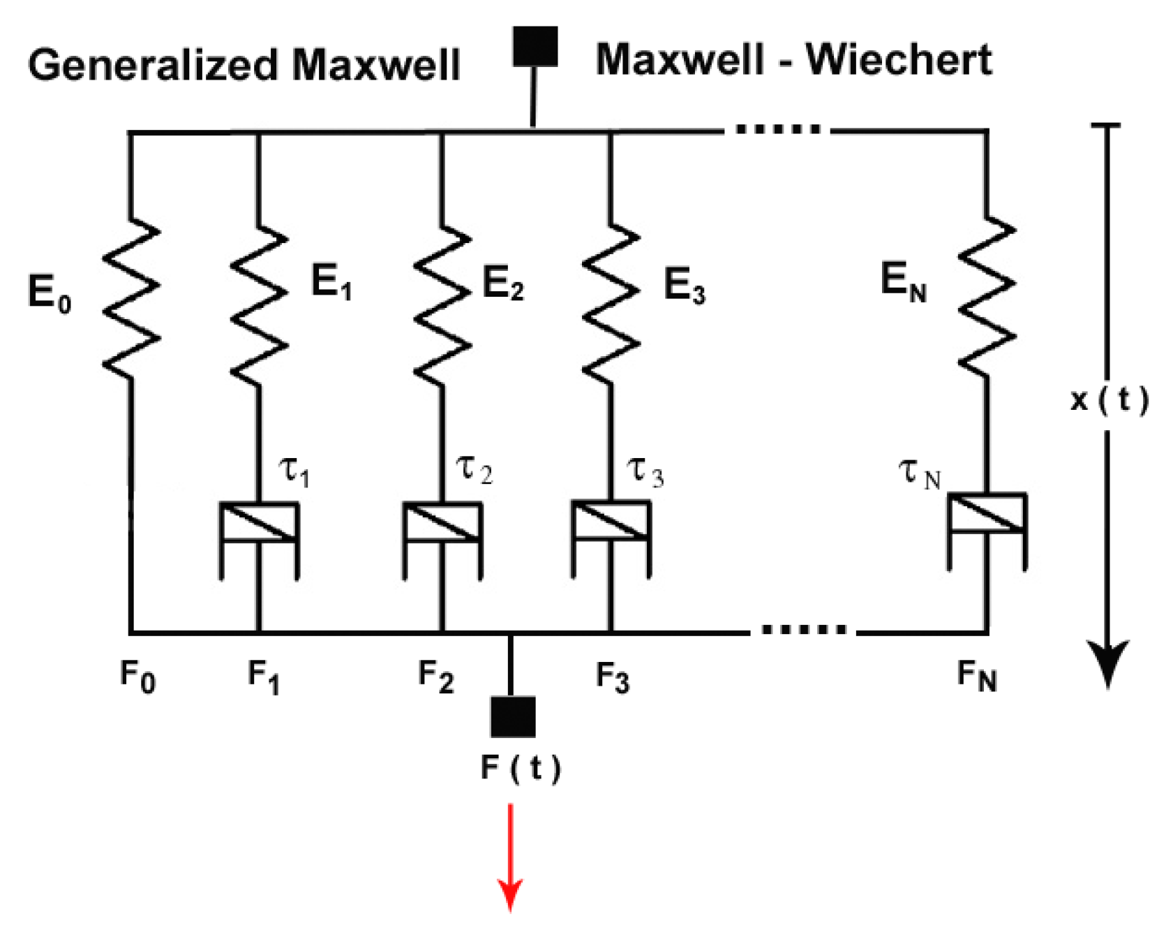
Thus, in such a case we have a summation of the effects of each spring-dashpot element, as in Maxwell–Wiechert models the elements are in parallel (see Figure 6), that is, , while the displacements are equal, that is, and .
Therefore, the total energy is a sum of all energies of the elements, namely,
Further, all calculation steps are the same as those already demonstrated for single exponential memory.
Note that in the Maxwell–Wiechert model there is one element without damping (i.e., just a spring) parallel to N elements consisting of a spring and a dashpot connected in a series. Thus, the result (83) is related only to elements with damping. The displacement of the single spring is simply Hook’s law , as the memory function is the Dirac’s delta, meaning that . Then, the spring’s energy is and should be added to the energy from (83). A good example concerning an exponential kernel of convolution integral equations exists in [25] (see Section 5.3, p. 73 in this book).
5.2. Fractional Element with Mittag-Leffler Memory
Consider the force–displacement causal relationship where the memory is the Mittag-Leffler function , namely,
(some properties of the Mittag-Leffler function are summarized in Appendix B.1), where
As supporting sources demonstrating the applicability of the (one-parameter) Mittag-Leffler function to model viscoelastic material behaviors, we refer readers to the comprehensive works of Enelund [35,36] and the real tests of Zhou et al. [37]; summarized information can be found in [30].
We now test the new construction of the causal relationship using a power-law force , leading to
Now, changing the order of the integral and the summation in (86), we obtain
5.2.1. Unit Step Force
For , we have a unit step force applied to the element and
Then, the energy is
5.2.2. Linear Ramp Force
For , we have a linear ramp force applied to the element and
Then, the energy is
5.2.3. Power-Law Ramp Force
In the general case with , the integration by parts was not easy to handle; thus, we applied computer algebra software (Maple) for the calculations. For , , and 10 terms of the Mittag-Leffler function, assuming for the sake of simplicity that , we obtain
For , we have , while for we have .
5.3. Fractional Element with Prabhakar Memory
With the Prabhakar memory kernel (A26), the general force–displacement relationship should be
For the sake of coherence, here we use the fractional order instead of in the definitions summarized in Appendix B.2.
The direct approach with the complete Prabhakar kernel is not an easy task; to avoid this problem for now and to make for an easier comparison of the results obtained up to this point, we use the long-time approximations (A29); an example of how to work with the complete Prabhakar function is provided in Section 5.3.3. Concerning the case with the first approximation (A29), we obtain
To a great extent, the kernel of this asymptotic resembles the power-law kernel of the Riemann–Liouville integral, which facilitates both the calculation and comparison of the final results.
In what follows, we solve two cases: a unit step and a linear ramp force.
5.3.1. Unit Step Force
In this specific case, the displacement is
Then,
and the energy of the fractional elements is
Positive energy growth requires that be obeyed, which is assured by the condition , with which the first of the asymptotic approximations (A29) is valid.
5.3.2. Linear Ramp Force
With the linear ramp force and applying integration by parts, we obtain
Consequently,
and the energy of the fractional element is
Positive growth requires that . This condition is supported by (A29), where .
5.3.3. An Example of the Use of the Complete Prabhakar Function
Let us now turn to the complete definition of the three-parameter Mittag-Leffler function, which for clarity of the following calculations can be presented as
Then, the Prabhakar function (A26) can be presented as
while the displacement can be defined in general as
In the case of a unite step function , the integration by parts in (107) yields
Thus, the energy of the fractional element is
For the linear ramp force , skipping the intermediate calculations, we obtain
5.4. Outcomes from the Examples Solved through Convolution Integrals with Memories Different from the Power Law
In general, the extension of the modeling approach applying more complex memory kernels can be considered a step towards generalization of the force–displacement relationships stemming from the causal formulation. This is a natural process in the modeling of nonlocal force–displacement relationships; the first step was carried out by Lorenzo and Hartley, with a simple example based on the Maxwell spring-dashpot model. Looking more deeply into the physics that this simple mechanical construction can model, it is apparent that the damping represented by the dashpot should strongly depend on the relaxation function of the medium on which the external force is exerted.
Moreover, taking into account the huge variety of material behaviors in the area of linear viscoelasticity (the Maxwell model belongs to this group) which do not obey the requirement of relaxation following the power law (modeled by the singular Abel kernel), it is reasonable to check whether other functions can model them [8]. If these functions are completely monotone (CM), then there is no harm in applying them in the nonlocal force–displacement relationship.
The examples developed in this section of the article have especially applied both new and old memory kernels (relaxation functions) known from the field of fractional calculus. This is a step beyond the level attained by Lorenzo and Hartley [6], and allows us to see how this can be done. The causal integral formulation allows controversial applications of the so-called fractional derivatives with kernels different from the classical Abel power law to be avoided [2,3], bypassing unfruitful discussions due to such operators (i.e., the so-called derivative) being convolution operators [25] that naturally appear during modeling of the nonlocal transport process [8,9].
From a calculation point of view, all these kernels yield results of the energy of the “modified” Maxwell’s models expressed as infinite series of power functions (as products of infinite series). Their practical calculation requires truncations of multiplicands upon imposed accuracy. As mentioned earlier this point of the calculation techniques is beyond the scope of this work; nevertheless, the problem is open and waiting for solutions, having remained open since the work of Lorenzo and Hartley [6], where there were no attempts made in this direction.
6. Final Comments
6.1. Outline of Main Achievements
In the end, we can strike a balance and outline what was attained as a development and contribution to the calculation of energies of fractional mechanical elements simply represented by Maxwell’s spring-dashpot construction. The first and foremost step in this study is the attempt to stress the causality principle as valid for all dynamic systems. This allows us to reconsider the approach of Lorenzo and Hartley and to demonstrate how the causal formulation works with examples taken from their original work. The extension, demonstrated in the case where the force is modeled by a generalized power-law ramp, allows us to see what problems emerge in the modeling and following calculations, with the examples of Lorenzo and Hartley as sub-cases.
The cases in which the causal integral formulation of the force–displacement relationship is solved by the application of more complex memory kernels is a step towards the correct application of fractional operators (with kernels different from Abel’s kernel) to dynamical systems. That is, constitutive fractional modeling in action requires knowledge about the physics prior to the use of nonlocal operators.
The standpoint expressed in Appendix A supports the author’s view of the application of the causality principle, and cannot be considered a complete study of the problem. The results obtained here allow further steps towards modeling both other mechanical rheological models and electrical circuits, taking into account the formal similarities between them [38].
6.2. Emergent Problems
Considering emerging problems, the author’s point of view is outlined, bearing in mind that questions and similar issues may be apparent to interested readers. To this end, the principal step that should be avoided in any future studies is the accuracy of calculation when model solutions involve infinite series. Last but not least, the correct model construction is of primary importance, with the Volterra integral equations (the force–displacement integral construction used here is a Volterra equation of the first kind) used rather than replacement by any fractional operator (derivatives).
6.3. Ideas Drawing New Problems
Many ideas might emerge from the developed problems for modeling and calculation techniques; several such targets can be envisaged, including:
- (a)
- Development of causal fractional modeling towards other mechanical models used in linear viscoelasticity.
- (b)
- Causal modeling of both linear and nonlinear electrical circuits, where the current–tension relationships closely resemble the force–displacement formulations covered here.
- (c)
- Causal fractional modeling of dissipative transport phenomena, where the flux-driving force or flux potential can be modeled by convolution integral relationships.
7. Conclusions
In this paper, causal modeling of a mechanical fractional element in the context of Maxwell spring-dashpot constructions has been developed, starting from the seminal work of Lorenzo and Hartley. The causal approach has been developed for various types of forces expressed as generalized power laws or series and memory kernels of Abel type and based on the Mittag-Leffler and Prabhakar functions. The causal integral formulation of the force–displacement relationship with complex memory kernels is a step towards the correct application of fractional operators (with kernels different from Abel’s kernel) to dynamical systems. The examples developed herein confirm this point of view.
Funding
This research received no external funding.
Data Availability Statement
Data is contained within the article.
Conflicts of Interest
The author declares no conflicts of interest.
Appendix A. The Causal Second Newton’s Law: A Point of View
The original formulation of Newton’s second law is that when a body is acted upon by a net force, the body’s acceleration multiplied by its mass is equal to the net force. Let us now consider two causal formulations with different physical backgrounds: a motion caused by the application of a net force to a body of mass m, and a force exerted by a moving body of mass m when it meets an object.
Appendix A.1. A Motion Caused by an Exerted Force
Let us consider the causal formulation of Newton’s second law when the motion is caused by a net force.
Through the Riemann–Liouville fractional integral, this can be formulated as
With this formulation, we assume a causal relationship between the momentum and the applied force , suggesting that the medium where this dynamic process takes place exhibits a power-law relaxation. Therefore, while there is no instant change in the momentum (output or the effect) after the force application (input or cause), there is a time shift. In the light of the memory kernel effects, we can say that the effects of the force on the changes in momentum are stronger for recent times than for past times, an effect that is well known from fractional calculus. The classical Newtonian law is memoryless and corresponds to the case , or in other words when the memory is represented by the Dirac delta function.
Now, using the properties and , where c is a scaling constant, and applying the operator to both sides of (A1), we obtain
It is worth noting that results (A2) and (A3) are natural consequences of the semi-group properties of the Riemann–Liouville fractional derivative and integral, that is, . However, Formulation (A1) is more general, as the memory integral may represent a more complex reaction of the medium where the dynamic process force displacement is taking place and the relaxation may be modeled by a function other than the power-law one. In such a case, there are guarantees that semi-groups exist.
Last but not least, for the sake of academic correctness it is necessary to mention that the general definition (A1) was used by Baleanu et al. [39] (as Equation (13) in this article), albeit the problem development was carried out mathematically in the sense of the Caputo derivative concerning a physical interpretation close to viscous interactions between layers in the classical mechanical interpretations of laminar flows. Starting from (A1), we can develop a fractional version of the Newtonian law in the sense of the Caputo derivative; however, we restrict ourselves to the Riemann–Liouville fractional integral following the line drawn by Lorenzo and Hartley, as well as the main line of this study that the formulation of the convolution (memory) integral in the cause–effect relationship is the primary step.
Remark A1.
This point of view on Newton’s second law only demonstrates how it can be interpreted in light of the causality principle. The integral Formulation (A1) follows the Volterra construction of the evolutionary equation. Though it is far from an extension of this fundamental law, it stresses that nothing happens instantly when the cause acts. This point of view only draws a line that might be followed when some basic physical law might be reconsidered from the point of view of the causality principle. Certainly, at the time when the law was formulated there were no mathematical expressions of the causal physical law, even though the philosophical background existed. From the physical point of view, the time shift, i.e., the relaxation process, could be neglected in the cause–effect relationship if the overall process time scale is much larger than the relaxation time, allowing the relationship to be formulated as memoryless. However, when such effects cannot be neglected, a necessary step is to apply a nonlocal formulation. This problem is challenging for many existing physical laws, as many modern technologies are based on processes where the relaxation times and the processing time scales are of the same order of magnitude.
Appendix A.2. A Force Caused by the Impact of a Moving Body on an Object
Next, we consider the physical situation if a force exerted on an object when it meets a moving body of mass m. The integral formulation applying the Riemann–Liouville integral in the case when we have to model the force exerted on an object by a body of a m and moving with a velocity is
that is, the force of impact depends on the recent velocity of the body rather than on its velocity in the past. With this formulation, we can explain why the impact is stronger when the body is moving through air and weaker when the medium is water: the dissipation of the kinetic energy modeled by the delayed effect of the body motion, which we express through convolution integrals, needs to use different relation functions in the two cases, that is, the memory kernel strongly depends on the physical problem being modeled. Now, applying the operator to both sides of (A4), we obtain
a formulation that is somewhat close to that of Lorenzo and Hartley, bearing in mind that the physical situations are different in nature. Moreover, to a certain extent (A5) is close to the result of Baleanu et al. [39].
Remark A2.
These two examples only show that the physical background and understanding is primary in the formulation of the causal expressions of physical laws. The relaxation of the medium in which the motion of the body takes place defines the memory function in the integral formulation of force–displacement or force–velocity relationships. In the case of the classical Newtonian formulation, there is an instant reaction (no memory) that can be attributed to the epoch when it was formulated. This is additionally valid for large times for which all relaxations can be neglected.
Appendix B. Properties of Functions Related to the Used Relaxation Kernels
Appendix B.1. Mittag-Leffler Function
Appendix B.1.1. Mittag-Leffler Function (One Parameter)
The Mittag-Leffler function is defined by a power series function that is convergent in the whole complex plane [40]:
This is an entire function which reduces to the exponential function for .
In the context of the work developed here, we are interested in the function
The Laplace transform of is
There are two commonly used asymptotic representations [40]:
Appendix B.1.2. Mittag-Leffler Function (Two Parameters)
The two-parameter of Mittag-Leffler type is defined as a series expansion:
From this definition, it follows that
Integration of the two-parameter Mittag-Leffler-Function:
Derivatives of the two-parameter Mittag-Leffler Function:
From the Riemann–Liouville definition of a fractional derivative, the fractional differentiation of (A10) is [41]
When , , and is an integer, we have
For , we have
Appendix B.1.3. Mittag-Leffler Function (Three Parameters)
The three-parameter Mittag-Leffler function is completely monotone (CM) for and precisely when [43].
which is an entire function of order and type .
For large arguments, i.e., for , there is an asymptotic approximation [43]
The differentiation of the generalized Mittag-Leffler function (A18) [41] through the product leads to
For , we have
Appendix B.2. Prabhakar Function
Prabhakar [42] studied a generalized Mittag-Leffler function, which we call the Prabhakar kernel:
The Laplace transform of for some particular values of the parameters is [41]
For , the Laplace transform and its inverse are [41]
The function is locally integrable and completely monotone if the conditions and are satisfied [43].
Asymptotically, for we have
The integral of for any and is
For , the differentiation of is
References
- Findley, W.N.; Lai, J.S.; Onaran, K. Creep and Relaxation of Nonlinear Viscoelastic Materials; North Nolland Publishing: Amsterdam, The Netherlands, 1976. [Google Scholar]
- Koeller, R.C. Application of fractional calculus to the theory of viscoelasticity. J. Appl. Mech. 1984, 51, 299–307. [Google Scholar] [CrossRef]
- Friedrich, C. Relaxation and retardation functions of the Maxwell model with fractional derivatives. Rheol. Acta 1991, 30, 151–158. [Google Scholar] [CrossRef]
- Heymans, N.; Bauwens, J.C. Fractal rheological models and fractional differential equations for viscoelastic behavior. Rheol. Acta 1994, 33, 210–219. [Google Scholar] [CrossRef]
- Lion, A. On the thermodynamics of fractional damping elements. Continum Mech. Thermodyn. 1997, 9, 83–96. [Google Scholar] [CrossRef]
- Lorenzo, C.F.; Hatley, T.T. Energy considerations for mechanical fractional-order elements. J. Comp. Nonlinear Dynam. 2015, 10, 011014. [Google Scholar] [CrossRef]
- Podlubny, I. Fractional Differential Equations; Academic Press: New York, NY, USA, 1999. [Google Scholar]
- Hristov, J. Constitutive fractional modeling. In Mathematical Modeling: Principle and Theory; Dutta, H., Ed.; AMS Series “Contemporary Mathematics”; American Mathematical Society: Providence, RI, USA, 2023; Volume 786, pp. 37–140. [Google Scholar] [CrossRef]
- Hristov, J. The fading memory formalism with Mittag-Leffler-type kernels as a generator of non-local operators. Appl. Sci. 2023, 13, 3065. [Google Scholar] [CrossRef]
- Mittelstaedt, P.; Weingartner, P.A. Laws of Nature; Springer: Berlin/Heidelberg, Germany, 2005. [Google Scholar]
- Nussenzveig, H. Causality and Dispersion Relations; Mathematics in Science and Engineering; Academic Press: New York, NY, USA, 1972; Volume 95. [Google Scholar]
- Nutting, P.G. A new general law of deformation. J. Franklin Inst. 1921, 191, 679–685. [Google Scholar] [CrossRef]
- Nutting, P.G. Deformation in relation to time, pressure and temperature. J. Franklin Inst. 1946, 242, 449–458. [Google Scholar] [CrossRef]
- Scott-Blair, G.W.; Reiner, M. The rheological law underlying the Nutting equation. Appl. Sci. Res. 1951, A2, 225–234. [Google Scholar] [CrossRef]
- Hartley, T.T.; Trigeassou, J.-C.; Lorenzo, C.F.; Maamry, N. Energy storage and loss in fractional-order systems. J. Comput. Nonlinear Dynam. 2015, 10, 061006. [Google Scholar] [CrossRef]
- Hartley, T.T.; Lorenzo, C.F. The initialization response of linear fractional-order systems with constant history function. In Proceedings of the ASME 2009 International Design Engineering Technical Conferences and Computers and Information in Engineering Conference. Volume 4: 7th International Conference on Multibody Systems, Nonlinear Dynamics, and Control, Parts A, B and C, San Diego, CA, USA, 30 August–2 September 2009; ASME: New York, NY, USA, 2009; pp. 1327–1332. [Google Scholar] [CrossRef]
- Malti, R.; Cois, O.; Aoun, M.; Levron, F.; Oustaloup, A. Energy of fractional order transfer functions. IFAC Proc. Vol. 2002, 35, 449–454. [Google Scholar] [CrossRef]
- Hilfer, R. Fractional Time evolution. In Applications of Fractional Calculus in Physics; Hilfer, R., Ed.; World Scientific: Singapore, 2000; pp. 89–116. [Google Scholar]
- Knopp, K. Theory and Application of Infinite Series; Hafner: New York, NY, USA, 1928. [Google Scholar]
- de Prony, G.R. Essai Experimentale at analitique. J. Ecole Polytech. 1795, 1, 24–76. [Google Scholar]
- Mauro, J.C.; Mauro, Y.Z. On the Prony representation of stretched exponential relaxation. Phys. A 2018, 506, 75–87. [Google Scholar] [CrossRef]
- Mandelbrot, S. Dirichlet Series: Principle and Methods; D. Reidel Publishing Co.: Dordrecht, The Netherlands, 1972. [Google Scholar]
- Titchmarsh, E.C. Introduction to the Theory of Fourier Integrals, 2nd ed.; Clarendon Press: Oxfors, UK, 1948. [Google Scholar]
- Watson, E.J. Laplace Transforms and Applications; Van Nostrand Reinholt Co.: New York, NY, USA; London, UK, 1981. [Google Scholar]
- Srivastava, H.M.; Buschman, R.G. Theory and Applications of Convolution Integral Equations; Springer: Dordrecht, The Netherlands, 1992. [Google Scholar]
- Coleman, B.; Noll, W. Foundations of linear Viscoelasticity. Rev. Mod. Phys. 1961, 33, 239–249. [Google Scholar] [CrossRef]
- Pipkin, A.C. Lectures on Viscoelasticity Theory, 2nd ed.; Sprimger: New York, NY, USA, 1972. [Google Scholar]
- Garbarski, J. The application of an exponentially-type function for the modeling of viscoelasticity of solid polymers. Polym. Eng. Sci. 1992, 32, 107–114. [Google Scholar] [CrossRef]
- Tschoegl, N.W. The Phenomenological Theory of Linear Viscoelastic Behaviour: An Introduction; Springer: New York, NY, USA, 1989. [Google Scholar]
- Hristov, J. Linear viscoelastic responses and constitutive equations in terms of fractional operators with non-singular kernels: Pragmatic approach, Memory kernel correspondence requirement and analyses. Eur. Phys. J. Plus 2019, 134, 283. [Google Scholar] [CrossRef]
- Widder, D.V. An Introduction to Transform Theory; Academic Press: New York, NY, USA, 1971. [Google Scholar]
- Hristov, J. Derivatives with non-singular kernels: From the Caputo-Fabrizio definition and beyond: Appraising analysis with emphasis on diffusion models. In Frontiers in Fractional Calculus; Bhalekar, S., Ed.; Bentham Science Publishers: Sharjah, United Arab Emirates, 2018; pp. 269–342. [Google Scholar]
- Caputo, M.; Fabrizio, M. A new definition of fractional derivative without singular kernel. Prog. Fract. Differ. Appl. 2015, 1, 73–85. [Google Scholar]
- Caputo, M.; Fabrizio, M. Applications of new time and spatial fractional derivatives with exponential kernels. Prog. Fract. Differ. Appl. 2016, 2, 1–11. [Google Scholar] [CrossRef]
- Adolfsson, K.; Enelund, M.; Olsson, P. On the fractional order model of viscoelasticity. Mech. Time-Depend. Mater. 2005, 9, 15–34. [Google Scholar] [CrossRef]
- Enelund, M.; Lesieutre, G.A. Time domain modeling of damping using anelastic displacement fields and fractional calculus. Int. J. Solids Struct. 1999, 36, 4447–4472. [Google Scholar] [CrossRef]
- Zhou, H.W.; Wang, C.P.; Han, B.B.; Duan, Z.Q. A creep constitutive model for salt rock based on fractional derivatives. Int. J. Rock Mech. Min. Sci. 2016, 48, 116–121. [Google Scholar] [CrossRef]
- Alsaedi, A.; Nieto, J.J.; Venktesh, V. Fractional electrical circuits. Adv. Mech. Eng. 2015, 7, 1–7. [Google Scholar] [CrossRef]
- Baleanu, D.; Golmankhaneh, A.K.; Golmankhaneh, A.K.; Nigmatulin, R.R. Newtonian law with memory. Nonlinear Dyn. 2010, 60, 81–96. [Google Scholar] [CrossRef]
- Mainardi, F. On some properties of the Mittag-Leffler function Eα(-tα) completely monotone for t > 0 with 0 < α < 1. Discret. Contin. Dyn. Syst. B 2014, 19, 2267–2278. [Google Scholar] [CrossRef]
- Kilbas, A.A.; Saigo, M.; Saxena, R.K. Generalized Mittag-Leffler function and generalized fractional calculus operators. Integral Trasforms Spec. Funct. 2004, 15, 31–49. [Google Scholar] [CrossRef]
- Prabhakar, T.R. A singular integral equation with a generalized Mittag-Leffler function in the kernel. Yokohama Math. J. 1971, 19, 7–15. [Google Scholar]
- Mainardi, F.; Garrappa, R. On complete monotonicity of the Prabhakar function and non-Debye relaxation in dielectrics. J. Comp. Phys. 2015, 293, 70–80. [Google Scholar] [CrossRef]
- Giusti, A.; Colombaro, I.; Garra, R.; Garrappa, R.; Polito, F.; Popolizio, M.; Mainardi, F. A practical guide to Prabhakar fractional calculus. Frac. Calc. Appl. Anal. 2020, 23, 9–54. [Google Scholar] [CrossRef]
Figure 1.
Maxwell spring-dashpot mechanical rheological model.
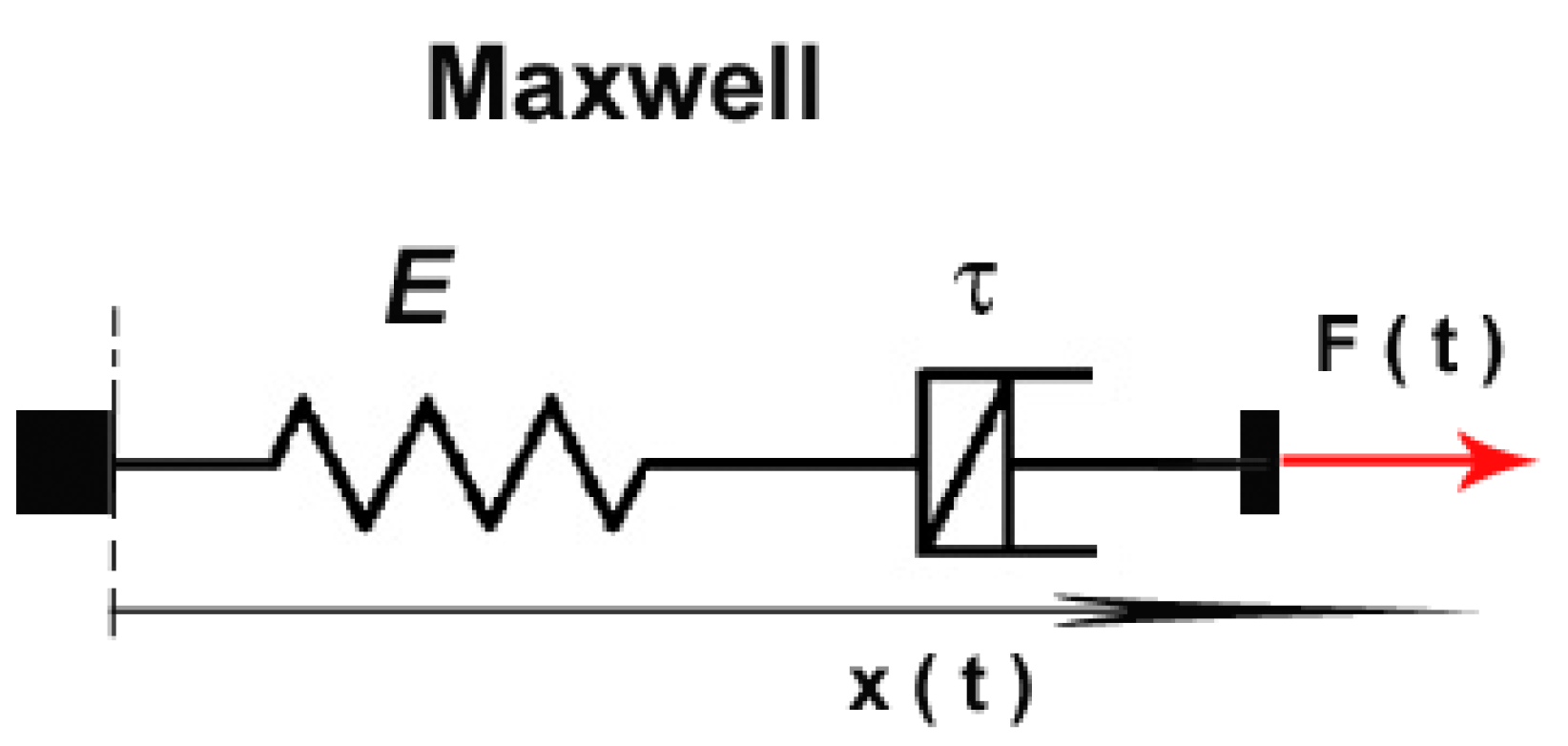
Figure 2.
Work (energy) of a fractional Maxwell element for the causal Formulation (3): (a) short times, (b) medium times, and (c) long times. The labels along the axes are the same as in the work of Lorenzo and Hartley [6], allowing for easy comparison of the results. The dashed lines correspond to .

Figure 3.
Work (energy) of a fractional Maxwell element for the causal Formulation (3) and a linear ramp force: (a) short times and (b) medium times. The labels along the axes are the same as in the work of Lorenzo and Hartley [6], allowing for easy comparison of the results. The dashed lines correspond to .
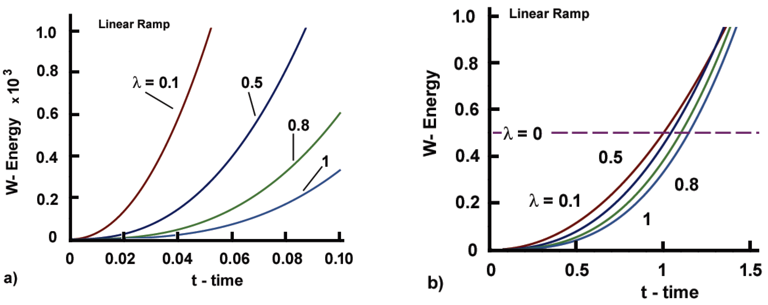
Figure 4.
Work (energy) of a fractional Maxwell element for the causal Formulation (3), singular power-law memory, and a power-law ramp force, following the results (38): (a) ; (b) ; (c) ; (d) .
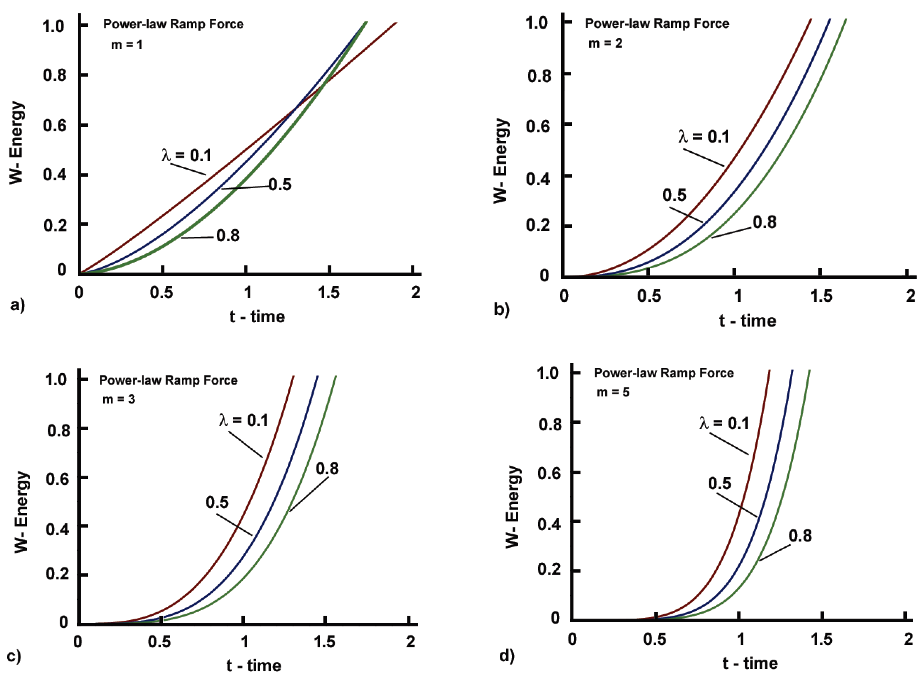
Figure 5.
Work (energy) of a fractional Maxwell element for the causal Formulation (3), singular power-law memory, and a power-law ramp force, following the results (38): (a) ; (b) ; (c) ; (d) 3D plot for .
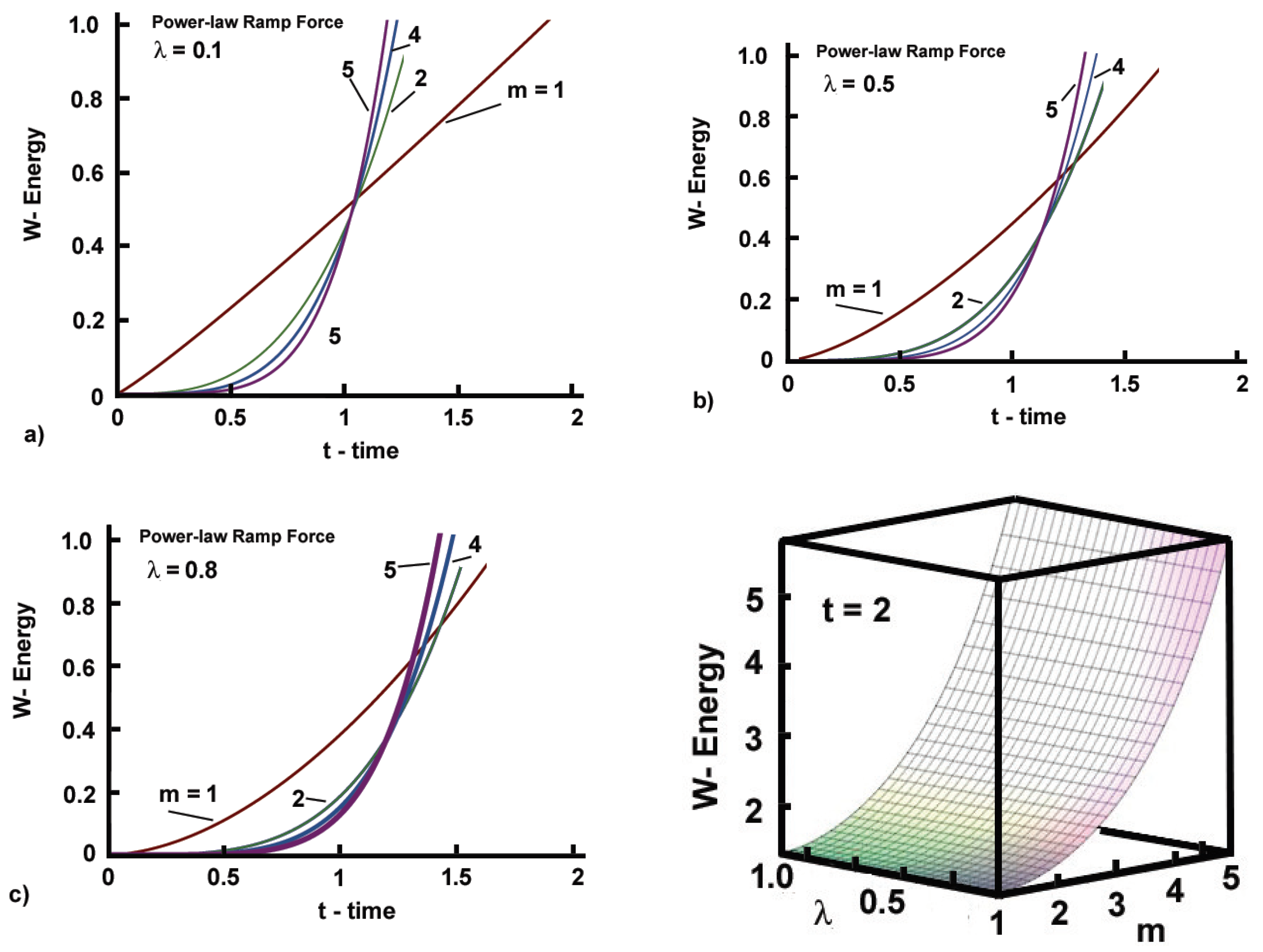
Figure 6.
Maxwell–Wiechert (Generalized Maxwell model) spring-dashpot mechanical rheological model.
Disclaimer/Publisher’s Note: The statements, opinions and data contained in all publications are solely those of the individual author(s) and contributor(s) and not of MDPI and/or the editor(s). MDPI and/or the editor(s) disclaim responsibility for any injury to people or property resulting from any ideas, methods, instructions or products referred to in the content. |
© 2023 by the author. Licensee MDPI, Basel, Switzerland. This article is an open access article distributed under the terms and conditions of the Creative Commons Attribution (CC BY) license (https://creativecommons.org/licenses/by/4.0/).
Share and Cite
MDPI and ACS Style
Hristov, J. Energies of Mechanical Fractional-Order Elements: Causal Concept and Kernel Effects. Appl. Sci. 2024, 14, 197. https://doi.org/10.3390/app14010197
AMA Style
Hristov J. Energies of Mechanical Fractional-Order Elements: Causal Concept and Kernel Effects. Applied Sciences. 2024; 14(1):197. https://doi.org/10.3390/app14010197
Chicago/Turabian StyleHristov, Jordan. 2024. "Energies of Mechanical Fractional-Order Elements: Causal Concept and Kernel Effects" Applied Sciences 14, no. 1: 197. https://doi.org/10.3390/app14010197
Note that from the first issue of 2016, this journal uses article numbers instead of page numbers. See further details here.