Article

Machinery Fault Signal Detection with Deep One-Class Classification

Department of Industrial and Management Engineering, Incheon National University, Incheon 22012, Republic of Korea
*
Author to whom correspondence should be addressed.
Appl. Sci. 2024, 14(1), 221; https://doi.org/10.3390/app14010221
Submission received: 25 November 2023 / Revised: 14 December 2023 / Accepted: 21 December 2023 / Published: 26 December 2023
(This article belongs to the Special Issue Artificial Intelligence in Fault Diagnosis and Signal Processing)

Abstract

:
Fault detection of machinery systems is a fundamental prerequisite to implementing condition-based maintenance, which is the most eminent manufacturing equipment system management strategy. To build the fault detection model, one-class classification algorithms have been used, which construct the decision boundary only using normal class. For more accurate one-class classification, signal data have been used recently because the signal data directly reflect the condition of the machinery system. To analyze the machinery condition effectively with the signal data, features of signals should be extracted, and then, the one-class classifier is constructed with the features. However, features separately extracted from one-class classification might not be optimized for the fault detection tasks, and thus, it leads to unsatisfactory performance. To address this problem, deep one-class classification methods can be used because the neural network structures can generate the features specialized to fault detection tasks through the end-to-end learning manner. In this study, we conducted a comprehensive experimental study with various fault signal datasets. The experimental results demonstrated that the deep support vector data description model, which is one of the most prominent deep one-class classification methods, outperforms its competitors and traditional methods.

1. Introduction

Modern industrial fields have furnished more complex and sophisticated machinery systems. However, unexpected faults in these machinery systems bring about significant losses in productivity and efficiency. To avoid the abrupt faults of machinery systems, preventive maintenance (PM) has been widely adopted as a maintenance strategy in various industrial fields [1,2]. These PM strategies attempt to conduct the maintenance (e.g., overhaul, refurbishment, and repair tasks) before the faults occur. In general, PM strategies can be divided into time-based maintenance (TBM) and condition-based maintenance (CBM) [3,4]. The TBM strategy periodically executes the maintenance activities in a predefined schedule. However, the TBM strategy often causes expensive maintenance costs because unnecessary maintenance activities are often performed [5]. Unlike, the CBM strategy performs maintenance tasks only when machinery fault symptoms are detected. Thus, it should entail a real-time diagnosis of the machinery status. Owing to its efficiency, CBM has received considerable attention in various industrial fields in recent years [5,6].
The CBM procedure comprises three main tasks: data acquisition, data processing, and fault diagnosis. (1) In the first step, sensor data that involve the health status of the machinery system are collected in real-time. (2) Then, to analyze the sensor data more easily, the collected raw data are preprocessed through feature engineering techniques. (3) Finally, using the preprocessed data, the machinery operating status is diagnosed, and maintenance is performed when the fault symptoms of the machinery systems are detected [1,7,8]. It is obvious that appropriately preprocessing the raw sensor data and accurately detecting the fault symptoms are fundamental prerequisites for a successful CBM strategy [9,10]. Therefore, the main purpose of this study is to propose a fault detection framework with deep neural network structures in order to implement a more efficient CBM strategy. The deep neural network structures are specialized to the feature engineering for given learning tasks [11,12]. Hence, the deep neural network-based approaches might show superior fault detection performance.
Most of the previous studies on machinery fault detection have used the sensor data obtained from both normal operating and fault statuses. However, the data from the fault status are not available in general because the fault rarely occurs in many real situations [13,14]. In addition, the operating status label information is not easy to obtain because it requires expensive analytical costs on machinery operating status. Therefore, in this study, we focus on the unsupervised deep neural network-based fault detection methods, which only use the sensor data obtained from normal operating status.
In recent years, various time-series signal data, including vibration, acoustic, and thermometric signals, have been widely used for fault detection [15,16]. These time-series signal data explicitly reflect machinery operating status, and it helps to more accurately detect the fault symptoms. Besides, owing to the rapid development of sensing and data storage techniques, a large amount of time-series signal data can be easily collected in real-time [8,17]. Therefore, utilizing these time-series signal data for fault detection has been spotlighted by a number of machinery operators. Then, a fault detection model can be constructed using one-class classification (OCC) methods. The OCC methods construct a decision boundary solely using time-series signal data obtained from only normal status (generally referred to as target signal), and the decision boundary finally determines whether a newly collected time-series signal was generated from normal status or not [18,19,20]. If the time-series signal is located outside the decision boundary, it is rejected as a fault signal, which is considered that the machinery fault might occur, and appropriate actions should be rapidly taken. Although the OCC methods have shown satisfactory performance in fault signal detection, they require an additional procedure that derives meaningful features from raw time-series signal data. This additional procedure is termed feature extraction.
The feature extraction attempts to generate several latent variables summarizing intrinsic properties of raw time-series signals. In most previous studies, manually created features (e.g., root mean square (RMS), kurtosis, and crest factor (CF)) have been widely utilized [21,22,23]. On the other hand, traditional feature learning techniques, including principal component analysis (PCA) [24] and kernel principal component analysis (KPCA) [25], have also been successfully used as feature extraction methods. The raw time-series signals are recorded at high sampling resolution and can be treated as high-dimensional data because individual values of the signal recorded at each time point can be regarded as variables. Thus, these traditional feature learning techniques entail dimensionality reduction to summarize the raw time-series signals of high dimensionality into smaller useful features. In spite of its simplicity, the manually crafted features simply summarize information of raw time-series signal data into a small number of values, and thus, it is difficult to reflect various characteristics of complex and noisy signals having nonstationary and nonlinear patterns [26,27]. For this reason, the manual feature creation may not be suitable for fault signal detection tasks. In addition, several traditional feature-learning techniques cannot accommodate the nonlinearity of target time-series signals, and kernel-based methods tend to be sensitive to the kernel function settings [28]. Finally, the feature creation or feature learning procedure is separately performed before fault detection model construction, and hence, the generated features may not be specialized for fault detection tasks [29].
To address these limitations, in recent years, deep neural network structures have been incorporated into OCC methods. In the deep neural network-based OCC methods (referred to as deep OCC methods), the feature extraction procedure is simultaneously performed with fault signal detection tasks in an end-to-end manner [11,12]. Thus, the deep neural network is basically designed to generate features optimized to a specified loss function of its corresponding task. Owing to the end-to-end manner’s advantage, deep neural network structures have been successfully used in OCC methods in recent years. Among various OCC methods, the boundary-based OCC methods (e.g., support vector data description (SVDD [30]) and one-class support vector machine (OCSVM [31])) have been the most widely combined with the deep neural network because their objective function can be easily reformulated for a loss function of the deep neural network. In the boundary-based methods, the objective function is formulated to construct a compact hypersphere enclosing the target class, and the hyperspheres can be used as a decision boundary to discriminate the fault signals from target signals. By doing so, optimized features through the deep neural network structure help build more sophisticated decision boundaries by accommodating the inherent patterns of target signals.
The following are the main contributions of this study:
  • The deep OCC methods can achieve superior fault detection performance, although raw time-series signals are directly used as input data. In general, for more effectively analyzing the time-series signals, signal processing techniques (e.g., short-time Fourier transform (STFT [32,33]) or wavelet transform [34]) are used to transform the raw signals. However, these signal-processing techniques require additional user-specified hyperparameters, which should be carefully determined. In contrast, the deep OCC methods do not need any signal processing techniques. This implies the efficiency of the deep OCC methods in handling the raw time-series signal data.
  • In the deep OCC methods, more useful features for fault signal detection can be simultaneously extracted along with minimizing loss function on anomaly detection tasks. By doing so, the fault signal detection performance can be improved.
  • Finally, we applied the deep OCC methods to the widely used benchmark fault signal datasets and the signal dataset collected from our own rolling element experimental platform. By doing so, the effectiveness and applicability of the deep neural network-based methods to real fault signal detection problems can be confirmed.
The remainder of this paper is organized as follows. Section 2 presents the related works on the proposed study. In Section 3, we present a deep neural network-based fault signal detection framework. The experimental settings, baseline of the comparison method, and results are reported in Section 4. The concluding remarks are provided in Section 5.

2. Related Works

This section deals with the details of existing OCC methods. Most of them are closely related to this study in that they can be used to fault signal detection problems. Later, we will consider most of the OCC methods introduced in this section for the various fault signal detection problems.

2.1. One-Class Classification Methods

Up to now, a number of OCC methods have been proposed, and they can be categorized according to the way to utilize the information on target signals, including density-based, ensemble-based, and boundary-based methods [19,20]. Among them, we focus on the boundary-based methods because they can generate more flexible decision boundaries through a nonlinear feature mapping function, and an objective function to build the optimal decision boundary can be explicitly formulated.
The SVDD is one of the most well-known boundary-based OCC methods. The SVDD attempts to find the most compact hypersphere to enclose as many target signal data as possible [30]. Then, if a signal falls outside of the hypersphere, it is rejected as a fault signal, and vice versa for the signal located inside of the hypersphere. However, if the hypersphere is constructed to involve all training target signals, the radius of the hypersphere might be too large, and too many fault signals are accepted as normal ones. To avoid the hypersphere being excessively large, the SVDD adopts slack variables, which allow a few training target signals to be located on the outer side of the hypersphere [30]. On the SVDD algorithm, the optimal hypersphere can be obtained as follows:
minmize R , a , ξ i   R 2 + C i = 1 n ξ i s . t .   ϕ x i a F k 2   R 2 + ξ i ,     i = 1 , , n ξ i   0 ,                                                       i = 1 , , n ,
where R2 is the radius of the hypersphere, a is the center of the hypersphere, and ξi denotes the slack variable of the i-th training target signal. In addition, C is a regularization parameter controlling the trade-off between the hypersphere’s volume and false positive error that rejects the target signal as fault signals, and ϕ is a nonlinear feature mapping function. The dual problem of Equation (1) can be formulated as follows:
maximize α   i = 1 n α i x i , x i i = 1 n j = 1 n α i α j x i , x j s . t .   0   α i C ,     i = 1 , , n     i = 1 N α i = 1 ,                     i = 1 , , n ,
where αi represents a Lagrange multiplier of the object xi and K〈 , 〉 denotes the kernel function corresponding to its own feature mapping function ϕ. After solving the dual problem presented in Equation (2), the new time-series signal (xnew) is classified as a normal or fault signal by calculating the distance between the new signal and the hypersphere center, ‖ϕ(xnew) − a2 [30]. If this distance is larger than R (i.e., the new signal falls outside the hypersphere), it is finally rejected as a fault signal.
Although the support vector-based methods are the most popular OCC methods, they are sensitive to the noisy patterns around the target class, and thus, when there are several noises in training data, the support vector-based methods cannot capture target class structures [19,20,35]. Moreover, they are still quite vulnerable to the model settings, including the kernel function choice or regularization hyperparameters [36,37].
In addition to boundary-based methods, density-based and ensemble-based methods have also been widely used for fault signal detection. The density-based methods estimate a density that quantifies the representativeness of the target signal, and a signal having a small density value is rejected as a fault signal. Generally, the density can be defined with a probability function, and thus, the density-based methods involve probability function estimation procedures. The kernel-density estimation (KDE [38]) is widely used to estimate the probability function along with target class structures, and this method defines the probability function as a weighted sum of the kernel function values centered at each training target signal. The contribution of each signal to the probability function is denoted by its kernel function value. This kernel function is computed by dividing the distance between signals with the bandwidth. In the KDE method, the bandwidth determines the shape of the kernel function and affects the smoothness of the estimated probability function. For small bandwidth, the kernel function has a high peak and narrow width, and the estimated probability function leads to a complicated decision boundary. Conversely, if the bandwidth value is too large, the kernel function may have a broad width, and the estimated probability function tends to generate a simple decision boundary.
On the other hand, ensemble-based methods have recently been proposed to overcome the fundamental limitations of the single-one class classifier. These methods construct multiple weak single one-class classifiers and aggregate them. By doing so, they help reflect various characteristics of the target signal using smaller subsets. Isolation forest (IsoForest [39]) is one of the most well-known ensemble-based methods, which builds many random isolation trees. Isolation trees recursively partition the target signals using random split conditions until the target signals are isolated in the individual isolation trees. IsoForest assumes that the fault signals require a small number of splits to be isolated because they have a different pattern than the target signal. By employing this approach, the anomaly score of IsoForest can be defined as the sum of the number of splits until it is isolated, and if the new signal has a small average number of splits, it is determined as a fault signal.
Although these traditional OCC methods have been well performed in the structured tabular data, for the unstructured data (e.g., time-series signal, image and video, and text-formatted data), appropriate features should be derived to apply them. However, these features obtained from independent feature extraction procedures to the OCC methods may not be specialized to detect anomalous patterns [40]. Hence, conventional OCC methods might not produce satisfactory fault signal detection performance in that the signal-typed data are the most representative unstructured data and require a careful feature extraction procedure.

2.2. Deep Neural Network-Based One-Class Classification Methods

As mentioned earlier, for more successful fault signal detection, features specialized for the fault signal detection tasks should be extracted. To this end, deep neural network structures, which are designed to generate optimized features for given learning tasks, have been successfully used for fault signal detection in recent years [11,12]. The deep neural network structure is composed of multiple intermediate layers (referred to as hidden layers) between input and output layers. These hidden layers generate features to minimize a loss function corresponding to the learning task without additional preprocessing or feature extraction procedures. Owing to this end-to-end learning manner, the deep neural network structure used for fault signal detection helps to achieve superior performance in that it can produce a specialized feature for anomalous signal detection tasks.
The deep neural network has been usually used for supervised learning tasks with numerous labeled data. However, in many real situations, fault signals obtained from machinery system faults or malfunctions rarely exist compared to the signals obtained from normal operating status, and thus, label information on the machinery operating condition might not be available [13,14]. Thus, these supervised deep neural networks cannot be used for fault signal detection tasks. For the unsupervised fault detection problem settings, unsupervised deep neural network-based OCC methods can be used. The unsupervised deep neural network-based OCC methods can be categorized as reconstruction-based [19,20], generative adversarial network (GAN)-based [41], and boundary-based methods, according to the way to generate the features of input signals.
Among them, the reconstruction-based OCC methods are based on autoencoder (AE)-based neural network structures. The AE-based neural network structures (e.g., stacked AE [11] and convolutional autoencoder (CAE [42,43])) attempt to generate meaningful features by reconstruction of the input signal data in the output layer. In the AE neural network, the input signals are embedded into smaller dimensions of latent features (referred to as encoding), and the latent features reconstruct the input signals (referred to as decoding). For a more accurate reconstruction of input signals into the output layer, the latent features should retain the intrinsic properties of input signals as much as possible. The stacked AE neural network [11] and CAE neural network [42,43] are the most widely used reconstruction neural network structures. These neural network structures can be used as OCC models by learning the neural network structures with only target signals (i.e., signals obtained from normal machinery status). Then, the errors between input signals and reconstructed outcomes can be used to calculate anomaly scores, quantifying the chances that the input signals are fault signals. That is to say; the target signals tend to have small reconstruction errors because the AE structures are constructed only using the training target signals. Conversely, the fault signals have larger reconstruction errors because the encoding structures are trained with no information on the fault signals, and the latent features cannot properly reconstruct the fault signals. In addition, the GAN-based OCC methods, which utilize neural network structures composed of both generator and discriminator, have recently been proposed. The generator attempts to create artificial signals as similar to input signals as possible, whereas the discriminator attempts to distinguish the artificial signals produced by the generator from the input signal as accurately as possible. Through an adversarial training scheme between the generator and discriminator, the GAN can produce artificial signals that have characteristics similar to target signals. Anomaly generative adversarial network (AnoGAN [44]), which is the most well-known GAN-based OCC method, is trained only using target signals, and thus, the generator produces a signal having similar patterns of normal operating status. Therefore, the generator can only generate an artificial signal similar to the training target signals, and the anomaly score of the newly collected signal is defined as the difference between the new signal and the generated signal from the generator of the AnoGAN. Finally, a signal having a large anomaly score is rejected as a fault signal. In addition to these methods, more recently, deep neural network structures have been successfully used for unsupervised anomaly detection problems in various unstructured datasets. For instance, Luo et al. proposed a sparse recurrent neural network (sRNN [45]) method to detect anomalous patterns in video datasets. Furthermore, self-supervised learning-based OCC methods have also been used for anomaly detection problems in image-formatted datasets [46,47].
Although these existing deep neural network-based OCC methods render reasonable results within the situations for which they were designed, no consensus exists regarding the best all-around performer in real situations. Firstly, reconstruction-based methods are designed to reproduce the original signal data simply by minimizing reconstruction errors. However, the reconstruction of the input signal might not be directly associated with the classification between target and fault signals [20,48]. Therefore, the reconstruction errors cannot be properly used as anomaly scores. Moreover, the GAN-based methods often generate inappropriate artificial signals because they often suffer from mode collapse problems [49]. The mode collapse problem is that the generator part tends to be trained to create only artificial signals with patterns that are almost similar to the most representative training target signal in order to minimize the discriminator’s loss. The mode collapse problem causes a lack of diversity of generated signals, and it eventually yields poor fault signal detection performance of the GAN-based OCC methods. Finally, the most recently proposed deep neural network-based OCC methods are designed for specific domains, such as anomaly video detection (sRNN) or unusual image detection (self-supervised approach-based methods). Therefore, these methods might not be properly utilized for fault signal detection problems.
To overcome the above limitations, we propose to use deep support vector data description (deep SVDD), the most well-known boundary-based method, for fault signal detection problems. The deep SVDD method has shown superior anomaly detection performance in various cases, only using the target class. Please note that Ruff et al. [50] have extended the deep SVDD methods as deep semi-supervised anomaly detection (deep SAD) methods, which use a limited number of anomaly samples. This deep neural network-based OCC method encourages the anomaly samples to be located outside the hypersphere as much as possible. By doing so, the decision boundary can be improved to discriminate between target class and anomaly. However, this method cannot be applied to the problem setting considered in this study, in which only the target class (i.e., time series signals collected from normal status) is available in the training phase. Therefore, we propose to use the deep SVDD as a fault signal detection method.

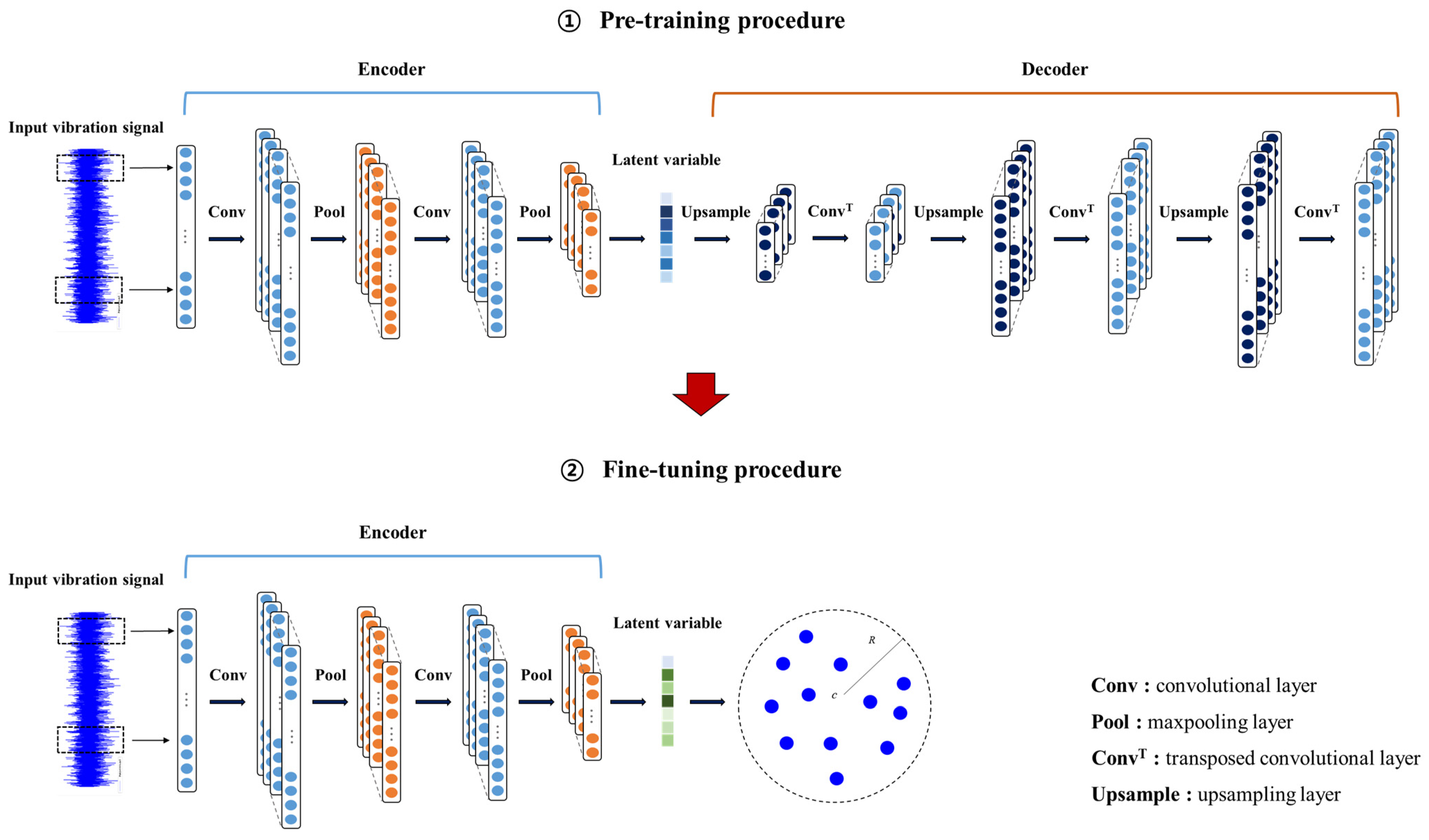
3. Fault Signal Detection with Deep Support Vector Data Description

In this study, we propose to utilize the deep SVDD method for the fault signal detection framework. Hence, this section presents a more detailed description of the deep SVDD method.
The deep SVDD [12] builds a hypersphere enclosing as many target signals as possible in the latent feature space generated by deep neural network structures. In the deep SVDD, the input time-series signal X R d (d denotes the dimension of time-series signal (i.e., the number of time points of the raw signal)) is mapped into the latent feature space F R p (p is the length of latent feature vector) as ϕ · ; W   :   X F , the neural network structures whose set of weights are W = W 1 , , W L . The W l denotes the weights of l -th hidden layer l 1 , , L (L represents the number of total hidden layers). In the deep SVDD, the latent feature space is analogous to the feature mapping function used in the traditional SVDD model, and the features obtained from training the deep SVDD model comprise the latent feature space. Thus, the deep SVDD attempts to generate better latent feature vectors where the optimal hypersphere can be constructed. The overall training procedure on the deep SVDD is illustrated in Figure 1.
As shown in Figure 1, the deep SVDD is trained by both pre-training and fine-tuning procedures. In order to more appropriately find the optimal latent feature space, deep SVDD first learns a stacked AE network as a pre-training procedure. The stacked AE network is composed of both encoding and decoding parts. The encoding part attempts to summarize the input time-series signal into smaller latent feature vectors, whereas the decoding part is used to reconstruct the input signals from the encoded latent feature vectors. The encoding part of the stacked AE is used as the initial network structure of the deep SVDD, and it helps the latent feature space can accommodate the intrinsic properties of the input time-series signal. By doing so, the initial weights of the neural network structure for the deep SVDD can be used to construct the hypersphere with a more accurate fault detection performance.
However, the stacked AE might not be localized characteristics of the time-series signal in that the hidden layers of the stacked AE are fully connected to each other. Hence, in this study, we propose to employ the one-dimensional CAE network instead of stacked AE because the one-dimensional CAE (1D-CAE) structures can successfully handle the time-series signal data owing to the convolutional layer and pooling layers [51,52]. In the 1D-CAE, the fully connected layers of the stacked AE are substituted as one-dimensional convolutional layers and pooling layers. The convolutional layer helps to consider localized properties within adjacent time points of input signals by using a convolutional kernel filter, and these convolutional kernel filters share weights across all regions of the input time-series signals. The output feature map of the j-th channel in the l -th convolutional layer, f j l , is calculated as follows:
f j l = σ m = 1 C l 1 f m l 1 W m ,   c l + b c l ,     c = 1 ,   2 ,   ,   C l ,     l = 1,2 , L ,
where f m l 1 is the output feature map of the m-th channel in the ( l -1)-th layer transformed by the kernel filter W m , c l of the c-th channel in the l -th layer. C l is the number of convolutional channels in l layer and b c l is the bias of c-th channel in the l -th layer. In addition, * is the convolutional operator, and σ(∙) denotes the nonlinear activation function. Hence, the output feature map having C l number of convolutional channels is computed. In general, each of the convolutional layers is followed by a pooling layer, which integrates adjacent values within the feature map into one value. Among various pooling manners, max-pooling, which picks the maximum value within a local region of the input feature map, is the most widely used. By employing the pooling layer, the size of the feature map and computational burden can be reduced. Both convolutional and max-pooling layer pairs (referred to as a convolutional block) can be repeated multiple times in the encoding part. At the end of the encoding part, the feature maps obtained by multiple convolutional blocks are flattened into a one-dimensional vector, and the flattened vector is finally mapped to a smaller latent features vector (dimension of latent feature vector (i.e., the number of latent features) is denoted as q) by the fully connected layer.
Then, in the decoding part, the input time-series signals are reconstructed from the latent variables of input time-series signals. The decoding part of the 1D-CAE comprises symmetrically arranged layers to the encoding part. In other words, the q-dimensional latent features vector is connected to a fully connected layer and reshaped into a one-dimensional feature map, and they are inversely reconstructed by transposed convolutional layers and up-sampling layers, which substitute the convolutional layers and max-pooling layers, respectively. The transposed convolutional layer expands the input feature map, conversely to the convolutional layer in the encoding part. The input feature map of the decoding part (i.e., the latent features vector) is transformed by a transposed convolutional layer as follows:
f ~ m l = σ m = 1 C l 1 f ~ m l 1 W ~ m , c l + b ~ c l ,     c = 1 ,   2 ,   3 ,   ,   C l ,     l = 1,2 , L ,
where ⊛ denotes the transposed convolutional operator which enlarges the input feature map, and f ~ m l 1 and f ~ m l represent the output feature map of the k-th channel in the ( l -1)-th layer and the c-th channel in the l -th layer, respectively. Further, W ~ m , c l denotes the transpose convolutional kernel filter of the c-th channel in the l -th layer and b ~ c l is the bias of the c-th channel in the l -th layer. All the weights of the 1D-CAE are obtained by minimizing the reconstruction errors between the input time-series signal and its reconstructed ones. The reconstruction error between input time-series signal, X , and reconstructed signals, X ~ , L X ,   X ~ , as follows:
L X ,   X ~ = 1 n i = 1 n X i X ~ i 2 ,
where X i and X ~ i are the i-th input time-series signal and its reconstructed outcomes, respectively, and n is the number of total input time-series signals. By the encoding part of the 1D-CAE, the initial latent feature vectors can retain the intrinsic properties of input time-series signals. Hence, the weight set in the encoding part, denoted as W , obtained from the 1D-CAE training procedure are used as initial weights of the deep support vector data description model ϕ · ; W .
Although the latent feature vector of the encoding part of the 1D-CAE neural network structure can accommodate intrinsic properties of training target time-series signals, it might not be optimized to detect anomalous signals. Thus, the deep neural network structure should be improved for fault signal detection tasks. To this end, the weight set W obtained from pre-training is updated to be optimized for the fault signal detection task. The deep SVDD performs subsequent fine-tuning procedures to minimize a loss function formulated for the fault signal detection task. The deep SVDD models can be divided into soft-boundary deep SVDD and one-class deep SVDD, according to how the loss function is defined.
(1)
Soft-boundary deep SVDD
In the Soft-boundary deep SVDD model, the loss function is defined as follows:
minimize R , W R 2 + 1 ν n i = 1 n m a x { 0 , ϕ x i ; W c 2 R 2 } + λ 2 l = 1 L W l F 2 ,
R represents the radius of hypersphere in the latent feature space, and ϕ x i ; W denotes the mapped signal to the q-dimensional latent feature space by neural network structures. In addition, c is the center of the hypersphere, and W represents the weight set of the neural network structures, W 1 , , W L . In this loss function, the first term minimizes R2 to find the smallest volume of the hypersphere that can enclose most of the target signal data. The second term is a slack term that allows for a few false positive errors that some mapped signals can be located outside the hypersphere. By adding the second term, the deep SVDD encourages the exclusion of a couple of anomalous target signals and prevents too many fault signals from being accepted as target signals. In this term, the slack hyperparameter ν 0,1 controls the trade-off between the size of the hypersphere and errors of the deep SVDD model. Finally, the third term is a weight decay regularizer for neural network weights W with the hyperparameter λ > 0, where · F 2 indicates the Frobenius norm. By adopting the third term, the overfitting problem of the deep neural network structures can be alleviated.
(2)
One-class deep SVDD
Under the assumption that the training data comprise only target signals, minimizing the size of the hypersphere enclosing most of the target signals in the latent feature space can be regarded as minimizing the average distances from the center of the hypersphere to the target signals. Thus, the first and second terms in the soft-boundary deep SVDD can be integrated as the sum of the average distance between the center and all training target signals in the latent feature space. Then, the one-class deep SVDD model can be formulated as follows:
minimize R , W 1 n i = 1 n ϕ x i ; W c 2 + λ 2 l = 1 L W l F 2 .
In the above equation, the first term attempts to minimize the average distance between the center and all training target signals in the q-dimensional latent feature space. Through this term, the neural network weights W can be updated to find latent feature space more specialized for fault signal detection in that it encourages the building of a compact decision boundary on the target signals. Compared with the soft-boundary deep SVDD, one-class deep SVDD can build ma more compact decision boundary by ignoring the slacks in Equation (5). Besides, the second term helps to prevent the overfitting risk, the same as the soft-boundary deep SVDD formulation. Finally, one-class deep SVDD does not require hyperparameter in that the first and second terms of the soft-boundary deep SVDD are integrated.
Please note that in the deep SVDD, the hypersphere center c should not be a free variable to prevent trivial solutions from having all zero values. That is to say, if the hypersphere center c is allowed to update during training of deep SVDD, c is estimated at zero values, and the hypersphere radius also nearly converges into zero. This problem is referred to as hypersphere collapse [12]. To avoid this problem, the hypersphere center c is calculated as the mean vector of the mapped signal ϕ x i ; W into the initial latent space obtained from the pre-training procedure for the encoding part of 1D-CAE. Once it is calculated, the hypersphere center c is then fixed during the fine-tuning procedure. In addition, we also do not employ bias terms and bounded activation functions to prevent the hypersphere collapse problem, as suggested by Ruff et al. [12].
After the deep SVDD structures are trained, they are finally used to determine whether newly collected signals are faulty or not. To this end, the anomaly score for the new signal x n e w , denoted as s( x n e w ) and quantified as follows:
s x n e w = ϕ x n e w ; W * c 2 ,
where W * are the optimal parameter derived from training deep SVDD, ϕ x n e w ; W * is the mapped signal x n e w into the q-dimensional latent feature space. If new signal x n e w having large anomaly score is deemed as a fault signals, and an appropriate action should be taken to cope with abnormality on the machinery status. Conversely, for the new signal having a small score, it is classified as a target signal, and any actions are not taken.

4. Experimental Study

4.1. Experimental Settings

To demonstrate the superiority of the deep SVDD model for the fault signal detection problems, we performed an experimental study with signal datasets in three cases. First, we utilized the two datasets provided by Case Western Reserve University (CWRU) and Paderborn University (PU), which are the most widely used benchmark fault signals used in a number of previous studies. In addition to these two benchmark datasets, we collected both vibration and acoustic signal datasets collected from our own rolling element experiment platform. In this study, we used the time series signals collected from rolling element bearing because the it is the most representative rotating machinery. Hence, through this experimental study, we demonstrated the applicability of the deep SVDD in real world machinery fault detection problems. More detailed description of each signal datasets are presented as follows:
Case 1: Case Western Reserve University (CWRU) dataset—Vibration signal (The CWRU benchmark dataset is available at: https://engineering.case.edu/bearingdatacenter/download-data-file (accessed on: 20 December 2023)).
The CWRU bearing dataset was collected from the accelerometer sensor attached to the bearing installed in fan end side of the test rig, as depicted in Figure 2.
In this study, we used the signal datasets collected by the accelerometer sensor attached in the fan end side. These benchmark signals are collected from various operating scenarios by changing the rotating speeds and vertical loads because vibration signals collected from different operating settings have different patterns. Table 1 shows the operating settings of four scenarios in the CWRU dataset.
The raw signals in this benchmark dataset were recorded at a sampling rate of 12,000 Hz per second (i.e., each raw signal was recorded as 12,000 time points per second). In addition, the dataset includes vibration signals from four types of bearing conditions: normal, inner race fault, outer race fault, and ball element fault. In these benchmark datasets, each fault type has four intensities corresponding fault diameters (e.g., 7 inch (weak fault), 14 inch (medium fault), 21 inch (strong fault)). Therefore, the CWRU dataset has ten bearing condition types, and signals from the normal condition are considered as target signals for OCC methods.
In this benchmark dataset, the ten vibration signals corresponding to each condition type were collected in approximately 10 to 20 s. In order to comprise the datasets having a sufficient number of signals to train the fault signal detection model, we segmented each raw signal into smaller ones. To this end, each raw signal is sliced in order for individual signals to have 1024 time points, and the sliced signals are overlapped each other with 768 time points. Then, the final fault signal detection model is constructed with the segmented signals. An example of these segmented signals to each bearing type is presented in Figure 3. As shown, the signals generated by the fault-bearing conditions have different patterns compared to the signals obtained from normal conditions. In addition, fault signal detection datasets of four scenarios in CWRU benchmark signal datasets are summarized in Table 2.
Case 2: Paderborn University (PU) dataset—Vibration signal (The PD benchmark dataset is available at: https://mb.uni-paderborn.de/kat/forschung/kat-datacenter/bearing-datacenter/data-sets-and-download (accessed on 20 December 2023)).
The Paderborn University dataset was collected by Lessmeier et al. [53]. This dataset is comprised of both vibration and current time series signals collected from the rolling bearing test rig shown in Figure 4.
The vibration signals are collected by the accelerometer sensor installed at the top end of the rolling bearing module. These benchmark signals are collected from various operating scenarios by changing (1) rotating speed, (2) radial force onto the bearing, and (3) load torque in the drive train because vibration signals collected from different operating settings have different patterns. Table 3 shows the operating settings of four scenarios in the PU dataset.
The dataset includes vibration signals from various types of bearing conditions: normal (Healthy), artificial inner race fault (AIR), artificial outer race fault (AOR), real inner race fault (RIR), and real outer race fault (ROR). In addition, the artificial fault types (AIR and AOR) are generated by electrical discharge machining (EDM), drilling, or electric engraver pitting, whereas real fault types (RIR and ROR) are made by accelerated life testing. Finally, among the six normal condition bearings having different operation times (bearing codes are K001, K002, K003, K004, K005, and K006), we employed the K003 bearing, which is operated for one hour. Hence, the normal signals obtained from K003 are used as target signals for OCC methods.
The raw signals in the PU dataset were collected for approximately 4 s at a sampling rate of 64,000 Hz per second (i.e., each raw signal was recorded 256,000 times). Thus, similar to the CWRU dataset, each raw signal is sliced in order for individual signals to have 2048 time points (no overlap between signals) to comprise the datasets having sufficient signals to train the fault signal detection model. Then, the final fault signal detection model is constructed with the segmented signals. An example of these segmented signals to each bearing condition type is presented in Figure 5.
As shown, the signals generated by the fault-bearing conditions have different patterns and scales compared to the signal obtained from normal conditions. In addition, fault signal detection datasets of four scenarios in PU benchmark signal datasets are summarized in Table 4.
Case 3: Rolling element experiment platform dataset—Vibration and acoustic signal
In addition to the benchmark datasets, we also collected both vibration and acoustic signals from our own rolling element-bearing experimental platform, presented in Figure 6.
In this bearing experimental platform, both the vibration and acoustic signals were simultaneously collected from the accelerometer sensor and preamplifier sensor, respectively, with a sampling frequency of 10,240 Hz per unit second. In this case, individual vibration and acoustic signals are collected per unit second. Hence, individual signals have 10,240-time points. In this experimental platform, a deep groove ball bearing is installed in the bearing housing of the simulator, and its sizes of inner side diameter, outer side diameter, and width are 35 mm, 72 mm, and 17 mm, respectively. In addition, the rotating speed of the bearing is 1200 RPM (revolutions per minute), and the vertical loader presses a bearing housing 150 kg (kilogram-force).
Similar to the CWRU dataset, the signals are collected from normal, inner race fault, outer race fault, and ball element fault conditions because these three faults are the most representative fault types [54,55]. These three faults in the bearing were generated by an electrical discharge machine. Furthermore, we also considered two fault intensity levels (i.e., strong and weak) by different defect diameters for each fault type because the signal patterns and amplitude scales differ from fault intensities. The examples of the vibration and acoustic signals collected from various bearing conditions are presented in Figure 7 and Figure 8, respectively.
The number of signals collected from both normal and all fault conditions is presented in Table 5.
In this study, we considered the traditional OCC methods as follows: SVDD, KDE, and IsoForest, which are the most representative boundary-based, probability distribution-based, and ensemble-based methods. For these traditional OCC methods, additional feature extraction procedures should be performed beforehand. To this end, we used three feature learning methods, principal component analysis (PCA), stacked autoencoder (stacked AE), and convolutional autoencoder (CAE). Then, we applied the SVDD, KDE, and IsoForest to the latent features obtained from those three methods. For the SVDD, we used the radius basis function (RBF) kernel having a parameter γ . In addition to γ , the traditional SVDD model requires other regularization hyperparameter C. In this study, we explored the hyperparameter pair (γ, C) within the given range: γ 2 10 , 2 9 , , 2 1 and C 0.01 , 0.02 , 0.03 , , 0.1 , respectively. For KDE, we also used a Gaussian kernel as the kernel function having bandwidth h, and the hyperparameter h was chosen within the range of h 2 0.5 , 2 1 , , 2 5 . Finally, for the IsoForest, we empirically selected the number of isolation trees, B, within the range of B 50 , 100 , 200 , 500 , 1000 . For these traditional OCC methods, we chose the optimal hyperparameter achieving the best performance within these candidate sets. The hyperparameter optimization for the OCC methods is not easy tasks because, as mentioned earlier, the fault detection is basically unsupervised problem settings [36,37]. In other words, in these problem settings, the label information is not available. To the best of our knowledge, there is lack of systematic ways to optimize the hyperparameters in fault detection problems. Hence, as in previous studies [35,56], we also picked the hyperparameters showing the highest AUROC values.
We also considered the following deep OCC methods for fault signal detection: reconstruction-based, GAN-based, and boundary-based methods. For the reconstruction-based methods, we trained stacked AE and CAE and computed the reconstruction error, x x ^ 2 , between the input signal (x) and reconstructed outcome ( x ^ ) as an anomaly score. In this study, we refer to these reconstruction-based OCC methods as anomaly scores with reconstruction errors of the stacked AE (ReSAE) and the CAE (ReCAE), respectively. For the GAN-based method, we utilized an AnoGAN-based convolutional neural network structure to more effectively handle the signal-formatted data. We set the number of latent features of the AnoGAN model as 256, as suggested by Schlegl et al. [44]. Finally, we applied the two deep SVDD models, soft-boundary deep SVDD and one-class deep SVDD, as boundary-based methods. In this study, we tried both stacked AE or CAE in the pre-training procedure of the deep SVDD model, in order to indicate the efficacy of convolutional blocks in order to analyze the signal data. In addition, to avoid the hypersphere collapse problem, we removed the bias term and used the leaky rectified linear unit activation function (Leaky ReLU). For the soft-boundary deep SVDD, we varied the hyperparameter ν within the range of ν 0.01,0.02 , 0.03 , , 0.1 , and selected one showed the best performance. The architecture details of the neural network structure for the deep SVDD are summarized in Table 6.
In the current study, the neural network hierarchy structures, such as the number of convolutional and pooling layers and the sizes of filters, are specified the same as in the original deep SVDD literature [12]. As suggested in [12], these network structures have shown reasonable results in various cases. Accordingly, we also adopted the same network hierarchy structures as [12]. Please note that the bounded activation functions, including the sigmoid and hyperbolic tangent functions, tend to cause the hypersphere collapse problem [12]. Therefore, we employed the Leaky ReLU, which is the most well-known unbounded activation function. As for the deep SVDD, this method is implemented by using open source code released to the public (The deep SVDD by using open source code available at: https://github.com/lukasruff/Deep-SVDD-PyTorch (accessed on 20 December 2023)). Finally, to conduct all experiments, we utilized an Intel® Core(TM) i5-9400F CPU @ 2.90 GHZ and NVIDIA GeForce RTX 2060 with 32 GB of RAM. All the DNN-based OCC methods were implemented with the GPU-accelerated Pytorch library (version 1.12.1) in Python (version 3.9.13).
As mentioned earlier, the training dataset consists of only normal signals, and the testing dataset is composed of the signals both in normal operating conditions and all fault types. To this end, we composed the training dataset as randomly selected 80% of the normal signals, and the testing dataset is composed of both all fault signals and the remaining 20% of the normal signals. Then, we evaluate the fault signal detection performance of each method through the area under the receiver operating characteristic curve (AUROC) on the testing dataset. The ROC (receiver operating characteristic) curve represents the trade-off between two types of errors, true positive and false positive, in fault signal detection problems. The true positive is the accuracy of classifying target signals as normal signals correctly, whereas the false positive is the error of classifying target signals as fault signals. It should be noted that a high true positive rate with a low false positive rate results under the large threshold values, while a low true positive rate with a high false positive rate results if the thresholds are set as small values. The ROC curve can be obtained by changing the threshold to make a false positive rate from zero to one. The AUROC is the area under the ROC curve, and the larger AUROC value indicates better fault signal detection performance.

4.2. Experimental Results

Table 7 shows the comparative results of the AUROC values of all OCC methods considered in the current study. We reported the averages and standard deviations of the AUROCs from 10 repetitions of random splitting of training/testing datasets. In this table, the highest average AUROC values are highlighted in bold.
Table 7 shows that the traditional OCC methods with independently performed feature extraction yielded lower AUROC values than deep neural network-based OCC methods. Those results indicate that separate feature extraction procedures might not generate specialized features for fault signal detection tasks. Conversely, the deep neural network-based OCC methods generally perform better than traditional OCC methods owing to their end-to-end learning manners for the fault signal detection tasks. In the deep neural network structures, latent features are optimized for fault signal detection tasks in that these features are simultaneously generated to minimize the loss functions for the fault signal detection tasks. Therefore, it confirms that deep neural network-based methods are more appropriate for detecting fault signals than traditional OCC methods with separate feature extraction procedures. However, in the AnoGAN model, the generator part may poorly generate artificial target signals due to the mode collapse problem, and it results in undesirable fault signal detection performance. Besides, the reconstruction-based methods, ReSAE and ReCAE, also cannot perform better than the deep SVDD models because the reconstruction error of the input signal might not directly quantify the anomalous level of the input signal. Hence, the weights of the stacked AE or CAE should be updated for more accurate fault signal detection tasks. Conversely, both one-class deep SVDD and soft boundary deep SVDD models outperform other deep neural network-based methods because the more specialized features of fault signal detection can be derived as minimizing loss functions for anomaly detection tasks. It should be noted that the pre-training with CAE performs better than those with stacked AE because convolutional layers of the CAE network help to draw temporal information of time-series signals because they combine the signal values within adjacent time intervals. Therefore, the initial neural network structures of the encoding part in CAE can accommodate the intrinsic properties of time-series signal data, and it eventually helps to build more accurate decision boundaries for detecting fault signals.
In addition, we conducted a post-analysis on performance differences through a nonparametric statistical method. We applied the Wilcoxon signed rank test [57] regarding the statistical difference in AUROC values among all the above 16 methods. Based on p-values over all methods, the null hypothesis of performance equivalence between CAE pre-trained one-class deep SVDD (the top-ranked method) and other ones is tested. The results of the Wilcoxon signed rank test are provided in Table 8.
As shown in Table 8, both the CAE pre-trained one-class deep SVDD and soft-boundary deep SVDD methods attained the best or second average rank. In addition, the null hypothesis of performance equivalence was rejected with a significance level of α = 0.01, and it implies that there is a significant difference in performance between the CAE pre-trained deep SVDD (proposed) and other methods. Consequently, these results denote that the proposed deep SVDD with CAE pre-training significantly outperformed the others. Finally, there is no statistical difference between the two deep SVDD methods pre-trained by CAE, which are not significant. In spite of their equivalent performance, we suggest using the one-class deep SVDD because it alleviates the difficulty of selecting the hyperparameter ν in the soft-boundary deep SVDD method.
In this study, we also conducted additional experimental studies to examine the effect of a number of latent features on the fault signal detection performance by varying the number of latent features from 16 to 256. The AUROC values over different numbers of latent features in all cases are presented in Figure 9.
As shown in Figure 9, the fault signal detection performance of the deep SVDD model rarely differs by changing the number of latent features. Therefore, we specified the number of latent features as 16 in order to prevent the overfitting problem and mitigate the computational burden of the deep SVDD model.
Finally, in order to demonstrate the advantage of the deep SVDD method regarding fault signal detection, we compared it with other feature extraction methods (PCA, AE, and one-dimensional CAE). To this end, we visualized these 16 latent features extracted from these four methods by facilitating the t-distributed stochastic neighborhood embedding (t-SNE [58]) technique. Figure 10 shows the two-dimensional t-SNE plots of latent features obtained from four feature extraction methods.
As shown in Figure 10, in the latent features obtained from PCA and AE, normal and fault signals are quite overlapped each other. The PCA cannot deal with the nonlinear patterns, and thus, it might not properly deal with the complex time series signal data. Moreover, in the AE, the layers are fully connected to each other, and these fully connected structures also cannot accommodate the temporal properties of the time series signals. For these reasons, these two feature extraction methods cannot accurately detect the fault signals. Conversely, the one-dimensional CAE and deep SVDD pre-trained by one-dimensional CAE more clearly discriminate the fault signals from normal ones than PCA and AE. These results indicate that one-dimensional CAE can more properly handle the time series signals because the convolutional blocks (i.e., convolutional-max pooling layer pair) in CAE help to consider the temporal properties of the time series signals [51,52]. On the other hand, latent features obtained from the deep SVDD more clearly separate the fault signals and normal signals than those from one-dimensional CAE. In the fine-tuning procedure of the deep SVDD, latent features are updated to be specialized for fault signal detection. Therefore, the deep SVDD method can generate more useful features for fault signal detection tasks than only using one-dimensional CAE.

5. Conclusions

In this study, we present a fault signal detection framework based on deep SVDD for the implementation of an efficient CBM strategy on machinery systems. To this end, we utilize the raw time-series signal because it directly reveals the health status of the machinery system. To handle the raw time-series signal data, the deep SVDD model is trained by one-dimensional CAE as a pre-training procedure, and the encoding part of the CAE structure is used as the initial network structure of the deep SVDD model.
The pre-training procedure helps to more accurately detect the decision boundary and the fault signals because intrinsic properties of time-series signal data can be accommodated to the neural network structures of the encoding part. Then, in the fine-tuning procedure, the neural network structures for the deep SVDD model are updated to minimize the loss function for the anomaly detection tasks. Through the fine-tuning procedure, the latent features specialized to the fault signal detection can be generated, and it eventually helps the deep SVDD model to achieve superior fault signal detection performance. To demonstrate the efficacy of the deep SVDD model in fault signal detection, we used a widely used benchmark signal dataset (CWRU dataset) and both the vibration and acoustic signal datasets collected from our own rolling element experiment platform. In this experimental study with these datasets, the deep SVDD model outperforms other OCC methods, and these results confirm the applicability of the deep SVDD model in real fault signal detection problems.
In spite of its superiority in fault signal detection problems, the decision boundary of the deep SVDD model might be corrupted by the noisy or outlying time series signals, which are generated by incomplete sampling or data transmission error [20,56]. Thus, in further study, we will address the deep SVDD model’s vulnerability against noisy or outlying time series signals. To this end, we will improve the deep SVDD model by incorporating the relative density of individual signals because these noisy or outlying time series signals tend to be located in sparse regions in feature space.

Author Contributions

D.Y. is responsible for the whole part of the paper (Conceptualization, methodology, formal analysis, validation, and writing—original draft preparation), and J.Y. is responsible for formal analysis, review and editing, supervision, and fund acquisition. All authors have read and agreed to the published version of the manuscript.

Funding

The corresponding author (J.Y.) of this research was supported by the Incheon National University (International Cooperative) Research Grant in 2021.

Institutional Review Board Statement

Not applicable.

Informed Consent Statement

Not applicable.

Data Availability Statement

The data presented in this study are available on request from the corresponding author. The data are not publicly available due to ongoing several other studies with the datasets presented in this study. If all of these studies are published, we will release the datasets presented in this study in our research team’s website.

Conflicts of Interest

The authors declare no conflicts of interest.

References

  1. Kumar, S.; Goyal, D.; Dang, R.K.; Dhami, S.S.; Pabla, B.S. Condition based maintenance of bearings and gears for fault detection–A review. Mater. Today Proc. 2018, 5, 6128–6137. [Google Scholar] [CrossRef]
  2. Kim, J.; Ahn, Y.; Yeo, H. A comparative study of time-based maintenance and condition-based maintenance for optimal choice of maintenance policy. Struct. Infrastruct. Eng. 2016, 12, 1525–1536. [Google Scholar] [CrossRef]
  3. Wu, S.; Zuo, M.J. Linear and nonlinear preventive maintenance models. IEEE Trans. Reliab. 2010, 59, 242–249. [Google Scholar]
  4. Yang, S.K. A condition-based failure-prediction and processing-scheme for preventive maintenance. IEEE Trans. Reliab. 2003, 52, 373–383. [Google Scholar] [CrossRef]
  5. Yang, B.S. An intelligent condition-based maintenance platform for rotating machinery. Expert Syst. Appl. 2012, 39, 2977–2988. [Google Scholar]
  6. Yang, S.K.; Liu, T.S. A Petri net approach to early failure detection and isolation for preventive maintenance. Qual. Reliab. Eng. Int. 1998, 14, 319–330. [Google Scholar] [CrossRef]
  7. Jardine, A.K.; Lin, D.; Banjevic, D. A review on machinery diagnostics and prognostics implementing condition-based maintenance. Mech. Syst. Signal Process. 2006, 20, 1483–1510. [Google Scholar] [CrossRef]
  8. Gao, Z.; Cecati, C.; Ding, S.X. A survey of fault diagnosis and fault-tolerant techniques—Part I: Fault diagnosis with model-based and signal-based approaches. IEEE Trans. Ind. Electron. 2015, 62, 3757–3767. [Google Scholar] [CrossRef]
  9. Goyal, D.; Pabla, B.S. Condition based maintenance of machine tools—A review. CIRP J. Manuf. Sci. Technol. 2015, 10, 24–35. [Google Scholar] [CrossRef]
  10. Lee, J.; Ardakani, H.D.; Yang, S.; Bagheri, B. Industrial big data analytics and cyber-physical systems for future maintenance & service innovation. Procedia CIRP 2015, 38, 3–7. [Google Scholar]
  11. Hinton, G.E.; Salakhutdinov, R.R. Reducing the dimensionality of data with neural networks. Science 2006, 313, 504–507. [Google Scholar] [CrossRef] [PubMed]
  12. Ruff, L.; Vandermeulen, R.; Goernitz, N.; Deecke, L.; Siddiqui, S.A.; Binder, A.; Müller, E.; Kloft, M. Deep One-Class Classification. In Proceedings of the International Conference on Machine Learning, Stockholm, Sweden, 10–15 July 2018. [Google Scholar]
  13. Li, W.; Shang, Z.; Gao, M.; Qian, S.; Zhang, B.; Zhang, J. A novel deep autoencoder and hyperparametric adaptive learning for imbalance intelligent fault diagnosis of rotating machinery. Eng. Appl. Artif. Intell. 2021, 102, 104279. [Google Scholar] [CrossRef]
  14. Shao, S.; Wang, P.; Yan, R. Generative adversarial networks for data augmentation in machine fault diagnosis. Comput. Ind. 2019, 106, 85–93. [Google Scholar] [CrossRef]
  15. Baydar, N.; Ball, A. Detection of gear failures via vibration and acoustic signals using wavelet transform. Mech. Syst. Signal Process. 2003, 17, 787–804. [Google Scholar] [CrossRef]
  16. Zhu, Y.; Li, G.; Tang, S.; Wang, R.; Su, H.; Wang, C. Acoustic signal-based fault detection of hydraulic piston pump using a particle swarm optimization enhancement CNN. Appl. Acoust. 2022, 192, 108718. [Google Scholar] [CrossRef]
  17. Zhang, J.; Sun, Y.; Guo, L.; Gao, H.; Hong, X.; Song, H. A new bearing fault diagnosis method based on modified convolutional neural networks. Chin. J. Aeronaut. 2020, 33, 439–447. [Google Scholar] [CrossRef]
  18. Krawczyk, B.; Woźniak, M.; Cyganek, B. Clustering-based ensembles for one-class classification. Inf. Sci. 2014, 264, 182–195. [Google Scholar] [CrossRef]
  19. Yu, J.; Kang, J. Clustering ensemble-based novelty score for outlier detection. Eng. Appl. Artif. Intell. 2023, 121, 106164. [Google Scholar] [CrossRef]
  20. Yu, J.; Do, H. Proximity-based density description with regularized reconstruction algorithm for anomaly detection. Inf. Sci. 2024, 654, 119816. [Google Scholar] [CrossRef]
  21. Lei, Y.; He, Z.; Zi, Y. A new approach to intelligent fault diagnosis of rotating machinery. Expert Syst. Appl. 2008, 35, 1593–1600. [Google Scholar] [CrossRef]
  22. Lei, Y.; Zuo, M.J. Gear crack level identification based on weighted K nearest neighbor classification algorithm. Mech. Syst. Signal Process. 2009, 23, 1535–1547. [Google Scholar] [CrossRef]
  23. Shen, Z.; Chen, X.; Zhang, X.; He, Z. A novel intelligent gear fault diagnosis model based on EMD and multi-class TSVM. Measurement 2012, 45, 30–40. [Google Scholar] [CrossRef]
  24. Abdi, H.; Williams, L.J. Principal component analysis. WIREs Comp. Stat. 2010, 2, 433–459. [Google Scholar] [CrossRef]
  25. Schölkopf, B.; Smola, A.; Müller, K.R. Kernel principal component analysis. In Proceedings of the International Conference on Artificial Neural Networks, Berlin, Germany, 8–10 October 1997. [Google Scholar]
  26. Lu, W.; Wang, X.; Yang, C.; Zhang, T. A novel feature extraction method using deep neural network for rolling bearing fault diagnosis. In Proceedings of the 27th Chinese Control and Decision Conference, Qingdao, China, 23–25 May 2015. [Google Scholar]
  27. Zhang, Y.; Zhou, T.; Huang, X.; Cao, L.; Zhou, Q. Fault diagnosis of rotating machinery based on recurrent neural networks. Measurement 2021, 171, 108774. [Google Scholar] [CrossRef]
  28. Hu, Z.; Zhao, H.; Peng, J. Low-rank reconstruction-based autoencoder for robust fault detection. Control Eng. Pract. 2022, 123, 105156. [Google Scholar] [CrossRef]
  29. Chalapathy, R.; Menon, A.K.; Chawla, S. Anomaly detection using one-class neural networks. arXiv 2019, arXiv:1802.06360. [Google Scholar]
  30. Tax, D.M.; Duin, R.P. Support vector data description. Mach. Learn. 2004, 54, 45–66. [Google Scholar] [CrossRef]
  31. Schölkopf, B.; Platt, J.C.; Shawe-Taylor, J.; Smola, A.J.; Williamson, R.C. Estimating the support of a high-dimensional distribution. Neural Comput. 2001, 13, 1443–1471. [Google Scholar] [CrossRef]
  32. Gröchenig, K. Foundations of Time-Frequency Analysis; Birkhäuser: Boston, MA, USA, 2001. [Google Scholar]
  33. Sejdić, E.; Djurović, I.; Jiang, J. Time–frequency feature representation using energy concentration: An overview of recent advances. Digital Signal Process. 2009, 19, 153–183. [Google Scholar] [CrossRef]
  34. Ogden, R.T. Essential Wavelets for Statistical Applications and Data Analysis; Birkhäuser: Boston, MA, USA, 1997. [Google Scholar]
  35. Chen, G.; Zhang, X.; Wang, Z.J.; Li, F. Robust support vector data description for outlier detection with noise or uncertain data. Knowl.-Based Syst. 2015, 90, 129–137. [Google Scholar] [CrossRef]
  36. Ghafoori, C.Z.; Erfani, S.M.; Rajasegarar, S.; Bezdek, J.C.; Karunasekera, S.; Leckie, C. Efficient unsupervised parameter estimation for one-class support vector machines. IEEE Trans. Neural Netw. Learn. Syst. 2018, 29, 5057–5070. [Google Scholar] [CrossRef]
  37. Yu, J.; Kang, S. Clustering-based proxy measure for optimizing one-class classifiers. Pattern Recognit. Lett. 2019, 117, 37–44. [Google Scholar] [CrossRef]
  38. Parzen, E. On estimation of a probability density function and mode. Ann. Math. Stat. 1962, 33, 1065–1076. [Google Scholar] [CrossRef]
  39. Liu, F.T.; Ting, K.M.; Zhou, Z.H. Isolation forest. In Proceedings of the IEEE International Conference on Data Mining, Pisa, Italy, 15–19 December 2008. [Google Scholar]
  40. Chen, L.; Xu, G.; Zhang, S.; Yan, W.; Wu, Q. Health indicator construction of machinery based on end-to-end trainable convolution recurrent neural networks. J. Manuf. Syst. 2020, 54, 1–11. [Google Scholar] [CrossRef]
  41. Goodfellow, I.; Pouget-Abadie, J.; Mirza, M.; Xu, B.; Warde-Farley, D.; Ozair, S.; Courville, A.; Bengio, Y. Generative adversarial nets. In Proceedings of the Advances in Neural Information Processing Systems, Montreal, QC, Canada, 8–13 December 2014. [Google Scholar]
  42. Aggarwal, C.C. Neural Networks and Deep Learning; Springer: New York, NY, USA, 2018. [Google Scholar]
  43. Masci, J.; Meier, U.; Cireşan, D.; Schmidhuber, J. Stacked convolutional auto-encoders for hierarchical feature extraction. In Proceedings of the International Conference on Artificial Neural Networks, Berlin, Germany, 14–17 June 2011. [Google Scholar]
  44. Schlegl, T.; Seeböck, P.; Waldstein, S.M.; Schmidt-Erfurth, U.; Langs, G. Unsupervised anomaly detection with generative adversarial networks to guide marker discovery. In Proceedings of the International Conference on Information Processing in Medical Imaging, Boone, NC, USA, 25–30 June 2017. [Google Scholar]
  45. Luo, W.; Liu, W.; Lian, D.; Tang, J.; Duan, L.; Peng, X.; Gao, S. Video anomaly detection with sparse coding inspired deep neural networks. IEEE Trans. Pattern Anal. Mach. Intell. 2019, 43, 1070–1084. [Google Scholar] [CrossRef]
  46. Bergman, L.; Hoshen, Y. Classification-based anomaly detection for general data. arXiv 2020, arXiv:2005.02359. [Google Scholar]
  47. Tack, J.; Mo, S.; Jeong, J.; Shin, J. Csi: Novelty detection via contrastive learning on distributionally shifted instances. In Proceedings of the Advances in Neural Information Processing Systems, Virtual Conference, 6–12 December 2020. [Google Scholar]
  48. Zong, B.; Song, Q.; Min, M.R.; Cheng, W.; Lumezanu, C.; Cho, D.; Chen, H. Deep autoencoding gaussian mixture model for unsupervised anomaly detection. In Proceedings of the International Conference on Learning Representations, Vancouver, BC, Canada, 30 April–3 May 2018. [Google Scholar]
  49. Metz, L.; Poole, B.; Pfau, D.; Sohl-Dickstein, J. Unrolled generative adversarial networks. arXiv 2016, arXiv:1611.02163. [Google Scholar]
  50. Ruff, L.; Vandermeulen, R.A.; Görnitz, N.; Binder, A.; Müller, E.; Müller, K.R.; Kloft, M. Deep semi-supervised anomaly detection. arXiv 2019, arXiv:1906.02694. [Google Scholar]
  51. Li, D.; Zhang, J.; Zhang, Q.; Wei, X. Classification of ECG signals based on 1D convolution neural network. In Proceedings of the IEEE International Conference on e-Health Networking, Applications and Services, Dalian, China, 12–15 October 2017. [Google Scholar]
  52. Yu, J.; Zhou, X. One-dimensional residual convolutional autoencoder based feature learning for gearbox fault diagnosis. IEEE Trans. Ind. Inf. 2020, 16, 6347–6358. [Google Scholar] [CrossRef]
  53. Lessmeier, C.; Kimotho, J.K.; Zimmer, D.; Sextro, W. Condition monitoring of bearing damage in electromechanical drive systems by using motor current signals of electric motors: A benchmark data set for data-driven classification. In Proceedings of the PHM Society European Conference, Bilbao, Spain, 5–8 July 2016. [Google Scholar]
  54. Liang, P.; Wang, W.; Yuan, X.; Liu, S.; Zhang, L.; Cheng, Y. Intelligent fault diagnosis of rolling bearing based on wavelet transform and improved ResNet under noisy labels and environment. Eng. Appl. Artif. Intell. 2022, 115, 105269. [Google Scholar] [CrossRef]
  55. Sun, J.; Liu, Z.; Wen, J.; Fu, R. Multiple hierarchical compression for deep neural network toward intelligent bearing fault diagnosis. Eng. Appl. Artif. Intell. 2022, 116, 105498. [Google Scholar] [CrossRef]
  56. Liu, B.; Xiao, Y.; Philip, S.Y.; Hao, Z.; Cao, L. An efficient approach for outlier detection with imperfect data labels. IEEE Trans. Knowl. Data Eng. 2013, 26, 1602–1616. [Google Scholar] [CrossRef]
  57. Conover, W.J. Practical Nonparametric Statistics, 3rd ed.; John Wiley & Sons: Hoboken, NJ, USA, 1999. [Google Scholar]
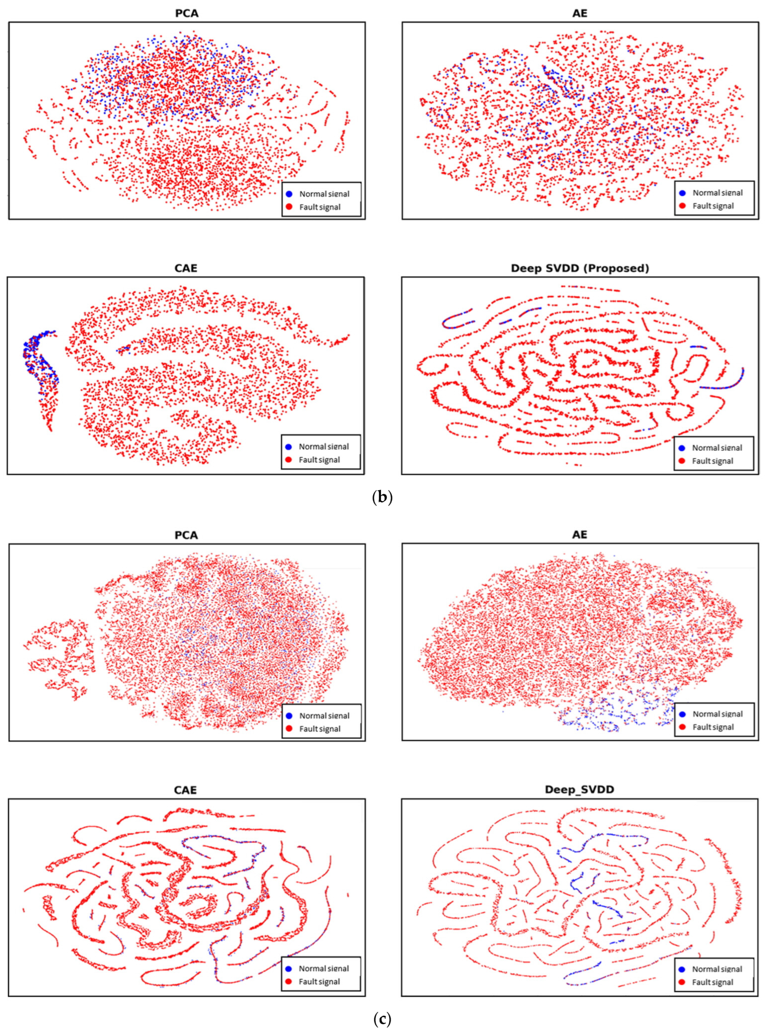
  58. Van der Maaten, L.; Hinton, G. Visualizing data using t-SNE. J. Mach. Learn Res. 2008, 9, 2579–2605. [Google Scholar]
Figure 1. Graphical illustration of fault signal detection process using the deep SVDD.
Applsci 14 00221 g001
Figure 2. Test rig for the CWRU dataset (This figure is available at: https://engineering.case.edu/bearingdatacenter/download-data-file (accessed on 20 December 2023)).
Applsci 14 00221 g002
Figure 3. Example segmented signals of all bearing conditions in Scenario 1 of CWRU datasets.
Applsci 14 00221 g003
Figure 4. Test rig for the PU dataset. It consists of five modules: (1) electric motor, (2) torque-measurement shaft, (3) rolling bearing test module, (4) flywheel, and (5) load motor [53].
Applsci 14 00221 g004
Figure 5. Example segmented signals of all bearing conditions in Scenario 1 of PU datasets.
Applsci 14 00221 g005
Figure 6. Rolling element experimental platform.
Applsci 14 00221 g006
Figure 7. Example of vibration signals obtained from our own rolling element experiment platform.
Applsci 14 00221 g007
Figure 8. Example of acoustic signals obtained from our own rolling element experiment platform.
Applsci 14 00221 g008
Figure 9. AUROC values over different numbers of latent features in (a) the CWRU dataset (Case 1), (b) the PU dataset (Case 2), and (c) the Rolling element experiment platform dataset (Case 3).
Applsci 14 00221 g009aApplsci 14 00221 g009b
Figure 10. Two-dimensional t-SNE plot of 16 latent features obtained from PCA, AE, CAE, and deep SVDD in (a) Scenario 1 of the CWRU dataset (Case 1), (b) Scenario 1 of the PU dataset (Case 2), and (c) vibration signals of Rolling element experiment platform dataset (Case 3).
Applsci 14 00221 g010aApplsci 14 00221 g010b
Table 1. Operating scenarios in CWRU benchmark signal datasets.
Rotating SpeedVertical Load
Scenario 11797 RPM0 HP (No pressure)
Scenario 21772 RPM1 HP
Scenario 31750 RPM2 HP
Scenario 41730 RPM3 HP
Table 2. The number of target and fault signals in CWRU benchmark signal datasets.
The Number of
Target Signals
(Normal Signals)
The Number of
All Fault Signals
Scenario 19526108
Scenario 218885160
Scenario 318925172
Scenario 418965180
Table 3. Operating scenarios in PU benchmark signal datasets.
Rotating SpeedRadial ForceLoad Torque
Scenario 11500 RPM1000 N0.7 Nm
Scenario 2900 RPM1000 N0.7 Nm
Scenario 31500 RPM1000 N0.1 Nm
Scenario 41500 RPM400 N0.7 Nm
Table 4. The number of target and fault signals in PD benchmark signal datasets.
The Number of
Target Signals
(Normal Signals)
The Number of
All Fault Signals
Scenario 1250051,660
Scenario 2
Scenario 3
Scenario 4
Table 5. The number of target and fault signals obtained from our own rolling element experiment platform.
Signal TypesThe Number of
Target Signals
(Normal Signals)
The Number of
All Fault Signals
Vibration485021,050
Acoustic
Table 6. Details of deep SVDD architecture.
CaseArchitectureBatch SizeOptimizer
(Learning Rate)
CWRU dataset
(Case 1)
8 × (5 × 1)-filters + max pooling + Leaky ReLU
4 × (5 × 1)-filters + max pooling + Leaky ReLU
Dense layer of 16 units
(i.e., the number of latent features (q) is 16)
32Adam optimizer ( η = 0.005)
PU dataset
(Case 2)
8 × (5 × 1)-filters + max pooling + Leaky ReLU
4 × (5 × 1)-filters + max pooling + Leaky ReLU
Dense layer of 16 units
(i.e., the number of latent features (q) is 16)
128
Rolling element experiment platform dataset
(Case 3)
8 × (5 × 1)-filters + max pooling + Leaky ReLU
4 × (5 × 1)-filters + max pooling + Leaky ReLU
Dense layer of 16 units
(i.e., the number of latent features (q) is 16)
128
Table 7. Average AUROC values of all OCC methods over ten time-series signal datasets (Scenario 1 to 4 of Case 1, Scenario 1 to 4 of Case 2, and vibration and acoustic signals of Case 3).
MethodsCWRU Dataset
(Case 1)
PU Dataset
(Case 2)
Rolling Element Experiment Platform Dataset
(Case 3)
Scenario 1Scenario 2Scenario 3Scenario 4Scenario 1Scenario 2Scenario 3Scenario 4Vibration
Signals
Acoustic
Signals
PCA + KDE1.000
(0.000)
0.986
(0.005)
0.992
(0.005)
0.993
(0.001)
0.340
(0.006)
0.790
(0.005)
0.780
(0.005)
0.827
(0.004)
0.665
(0.005)
0.603
(0.009)
PCA + IF0.995
(0.002)
0.994
(0.000)
0.994
(0.000)
0.994
(0.000)
0.349
(0.036)
0.782
(0.007)
0.778
(0.013)
0.822
(0.004)
0.722
(0.003)
0.618
(0.004)
PCA + SVDD1.000
(0.000)
0.994
(0.000)
0.994
(0.000)
0.994
(0.000)
0.393
(0.101)
0.791
(0.005)
0.776
(0.017)
0.825
(0.004)
0.735
(0.003)
0.637
(0.005)
AE + KDE0.883
(0.172)
0.548
(0.047)
0.524
(0.031)
0.391
(0.054)
0.681
(0.015)
0.730
(0.036)
0.733
(0.024)
0.748
(0.023)
0.519
(0.113)
0.534
(0.023)
AE + IF0.870
(0.168)
0.084
(0.097)
0.092
(0.102)
0.122
(0.044)
0.707
(0.009)
0.748
(0.012)
0.749
(0.013)
0.746
(0.008)
0.264
(0.124)
0.551
(0.025)
AE + SVDD0.858
(0.159)
0.286
(0.118)
0.530
(0.085)
0.535
(0.084)
0.717
(0.011)
0.684
(0.057)
0.650
(0.082)
0.700
(0.042)
0.412
(0.165)
0.530
(0.038)
CAE + KDE0.978
(0.028)
0.993
(0.001)
0.993
(0.001)
0.993
(0.002)
0.987
(0.001)
0.847
(0.054)
0.869
(0.015)
0.867
(0.054)
0.921
(0.009)
0.801
(0.042)
CAE + IsoForest0.962
(0.072)
0.998
(0.036)
0.988
(0.036)
0.974
(0.072)
0.980
(0.002)
0.860
(0.046)
0.883
(0.026)
0.870
(0.061)
0.924
(0.009)
0.819
(0.061)
CAE + SVDD0.976
(0.047)
0.985
(0.042)
0.999
(0.001)
0.974
(0.072)
0.980
(0.004)
0.877
(0.038)
0.895
(0.024)
0.882
(0.056)
0.794
(0.048)
0.622
(0.070)
ReSAE0.992
(0.001)
0.996
(0.002)
0.996
(0.003)
0.994
(0.000)
0.068
(0.011)
0.347
(0.022)
0.320
(0.017)
0.358
(0.024)
0.809
(0.038)
0.569
(0.021)
ReCAE0.999
(0.002)
0.999
(0.001)
0.998
(0.002)
0.998
(0.001)
0.048
(0.001)
0.327
(0.003)
0.303
(0.002)
0.333
(0.003)
0.732
(0.002)
0.569
(0.007)
AnoGAN0.765
(0.024)
0.567
(0.036)
0.570
(0.037)
0.604
(0.095)
0.216
(0.116)
0.452
(0.139)
0.399
(0.101)
0.417
(0.207)
0.722
(0.014)
0.691
(0.042)
Soft-boundary deep SVDD
(AE pre-trained)
0.980
(0.005)
0.994
(0.003)
0.985
(0.002)
0.989
(0.003)
0.792
(0.007)
0.823
(0.007)
0.760
(0.004)
0.791
(0.007)
0.819
(0.079)
0.643
(0.091)
One-class deep SVDD
(AE pre-trained)
0.980
(0.005)
0.993
(0.003)
0.985
(0.003)
0.988
(0.004)
0.775
(0.005)
0.793
(0.007)
0.762
(0.003)
0.759
(0.006)
0.859
(0.103)
0.683
(0.028)
Soft-boundary deep SVDD
(CAE pre-trained; Proposed)
0.985
(0.026)
1.000
(0.000)
1.000
(0.000)
1.000
(0.000)
0.991
(0.001)
0.936
(0.007)
0.941
(0.008)
0.940
(0.007)
0.985
(0.002)
0.912
(0.011)
One-class deep SVDD
(CAE pre-trained; Proposed)
1.000
(0.000)
1.000
(0.000)
1.000
(0.000)
1.000
(0.000)
0.991
(0.001)
0.939
(0.006)
0.944
(0.002)
0.939
(0.009)
0.985
(0.004)
0.922
(0.014)
Table 8. Wilcoxon signed-rank test results.
MethodsAverage Rankp-ValueHypothesis
(α = 0.01)
One-class deep SVDD (CAE pre-trained; Proposed)1.1--
Soft-boundary deep SVDD (CAE pre-trained; Proposed)1.90.1056Not reject
CAE + IsoForest5.90.0059Reject
CAE + KDE6.00.0058Reject
CAE + SVDD6.70.0020Reject
PCA + SVDD6.80.0089Reject
Soft-boundary deep SVDD (AE pre-trained)7.80.0020Reject
PCA + IF7.90.0058Reject
One-class deep SVDD (AE pre-trained)8.20.0020Reject
PCA + KDE8.60.0092Reject
ReSAE9.90.0059Reject
ReCAE10.00.0059Reject
AnoGAN12.70.0020Reject
AE + KDE13.10.0020Reject
AE + IF13.50.0020Reject
AE + SVDD13.60.0020Reject
Disclaimer/Publisher’s Note: The statements, opinions and data contained in all publications are solely those of the individual author(s) and contributor(s) and not of MDPI and/or the editor(s). MDPI and/or the editor(s) disclaim responsibility for any injury to people or property resulting from any ideas, methods, instructions or products referred to in the content.

