Testing the Reliability of Maximum Entropy Method for Mapping Gully Erosion Susceptibility in a Stream Catchment of Calabria Region (South Italy)

Abstract

Gully erosion poses severe problems for land degradation in several areas worldwide. This study aims to evaluate the accuracy and robustness of the maximum entropy (MaxEnt) method for assessing gully erosion susceptibility. We selected the catchment of the Mesima stream as the test site, which is situated in the southwest sector of the Calabria region (South Italy). An inventory map of gully erosion was realised and 12 predisposing factors, such as lithology, soil texture, soil bulk density, land use, drainage network, slope gradient, aspect, length–slope (LS), plan curvature, stream power index (SPI), topographic position index (TPI), and topographic wetness index (TWI), were selected to implement the dataset in the MaxEnt method. The accuracy and uncertainty of the method were tested by 10-fold cross-validation based on accuracy, kappa coefficient, and receiver operating characteristic curve (ROC) and related area under curve (AUC). The dataset was randomly divided into 10 equal-sized groups (folds). Nine folds (90% of the selected dataset) were used to train the model. Instead, the remaining fold (10% of the dataset) was used for testing the model. This process was repeated 10 times (equal to the number of the folds) and each fold was used only once as the validation data. The average of 10 repeated processes was performed to generate the susceptibility map. In addition, this procedure allowed the reliability of the susceptibility map to be assessed, in terms of variables, importance and role of predisposing factors selected, prediction ability, and accuracy in the assessed probabilities for each pixel of the map. In addition to exploiting the 10-fold cross-validation, the mean value and standard deviation for the probability estimates of each pixel were computed and reported in the susceptibility and uncertainty map. The results showed that the MaxEnt method has high values of accuracy (>0.90), of the kappa coefficient (>0.80), and AUC (>0.92). Furthermore, the achieved findings showed that the capacity of the method used for mapping gully erosion susceptibility is quite robust when the training and testing sets are changed through the 10-fold cross-validation technique.

1. Introduction

Gully erosion is a geomorphic process that affects landscape evolution [1,2,3] and can be considered the main process of sediment production within small watersheds [4,5,6]. Gullying phenomena are recognised as one of the leading causes of land degradation in many countries worldwide, causing massive loss of soil, severe economic devaluation, and heavy impacts on ecosystem services [3,7,8,9,10]. In the last decades, gully development was favoured by the combination of extreme rainfall events and unsuitable land use changes, such as converting forests to cultivated areas or uncontrolled deforestation and agriculture activities [10,11].

The gully erosion processes significantly affect several countries in the Mediterranean area, causing soil degradation and impacts on agriculture production, vital resources, and benefits of human beings [10,11,12,13,14,15]. For instance, many zones of the Calabria region (Southern Italy) are notably affected by intense water erosion processes as gullying phenomena, giving rise to serious soil loss every year [16,17,18]. In this regard, detecting the likely prone areas to gullying development is fundamental in directing land conservation strategies and sustainable progress [11,19].

Implementing the prediction models for mapping gully erosion susceptibility is one of the most important challenges in assessing potential risks and reducing negative impacts on the land. Gullies’ formation and spatial distribution are controlled by the complex interactions of a large variety of geo-environmental factors, including geology, soil, topography, rainfall, land cover, land use, and human activities [1,20,21,22,23,24]. Thus, the core principle of gully erosion susceptibility modelling is quantifying the interplay between gullies’ spatial distribution and the geo-environmental variables affecting these phenomena.

In the last decade, many statistical and machine learning methods combined with geographic information systems (GIS) and remote sensing technologies were proposed for evaluating and mapping gully erosion susceptibility in several areas worldwide [13,23,25,26]. The main bi- and multi-variate statistical methods employed in the previous research are frequency ratio [27], evidential belief function [28], certainty factors [29], information value [28], index of entropy [28], weights of evidence [30], logistic regression [25], and geographically weighted regression [13,31]. Instead, among the most known machine learning methods, there are random forest [32], artificial neural networks [22,33], support vector machine [33], boosted regression tree [32], and maximum entropy [20,34]. Moreover, machine learning methods are often identified as the most reliable methods for mapping gully erosion susceptibility [26,35].

In this context, this work aims to test the reliability of the maximum entropy machine learning method combined with GIS-based tools for mapping gully erosion susceptibility in the Mesima catchment, Calabria region (South Italy). In the Mesima basin, geomorphic processes, like gullying, periodically cause considerable soil erosion. Therefore, it becomes crucial to map the future gully erosion-prone areas to mitigate the adverse effects of these processes and for suitable land management, especially for agricultural areas.

2. Study Area

The modelling framework was calibrated and tested within the Mesima stream catchment, located in the southwestern portion of the Calabria region (South Italy), between 4,284,943 m N and 4,262,983 m N of latitude and 590,786 m E and 615,866 m E of longitude (Figure 1a). The catchment covers a surface of 173.5 km² with an altitude varying from 42 to 939 m. a.s.l. (Figure 1b). The drainage network is well developed, showing a hierarchy equal to the seventh order with a sub-dendritic drainage pattern and a hypsometric curve with a concave–convex shape indicating a high predisposition to undergo intense denudation processes [36].

Climatically, the catchment is affected by a Mediterranean climate, with mild and wet winters and hot and dry summers. The total annual rainfall ranges from 785 to 1572 mm, with a mean yearly precipitation of approximately 973 mm. The maximum rain usually occurs in January and December, while the minimum is between July and August.

Geologically, the study area is situated in a tectonic depression named Mesima graben, which constitutes the middle portion of the Calabrian–Peloritan Arc [37,38]. The graben is bounded by NE–SW trending normal faults and filled by Plio-Pleistocene marine and continental deposits, which cover the Paleozoic crystalline-metamorphic rocks or the Miocenic sedimentary rocks [36,37]. Palaeozoic crystalline-metamorphic rocks of the Capo Vaticano promontory and the Serre Massif, respectively, bound the western and eastern graben flanks [36,37,39].

The lithology in the Mesima catchment is mainly dominated by Pliocene silty clay deposits and secondarily from Pliocene sand, sandstone deposits, and conglomerate of Pleistocene. Locally, evaporitic limestones (Miocene in age) overlain in discontinuity in the gneiss and granite of the Paleozoic basement are intensely fractured and weathered [39,40]. Intense weathering processes due to marine aerosol also affect sedimentary deposits, mainly those close to coastal areas [41]. In some areas, eluvial–colluvial deposits (Holocene) overlay the sedimentary rocks or, directly, the crystalline-metamorphic rocks. Finally, Holocene alluvial deposits dominate the valley floors.

The morphology of the landscape is characterised mainly by hillslopes with undulating sharp and rounded slopes, generally with V-shaped valleys. The latter only assumes a more concave form when colluvial deposits partly fill them. The slope gradient ranges from 0° to 77°, with an average value of about 13.7°. Badlands often affect the silty clay slopes because of water erosion caused by ephemeral streams. Instead, more competent rocks (sandstone and/or conglomerates) locally generate high-gradient slopes or sub-vertical escarpments involved in widespread landslides [36,42]. The catchment is boarded by terrace surfaces in the upper and middle sectors, representing the relics of old fluvial terraces [36,37]. Quaternary tectonic activity [37] shaped landforms, giving rise to a dense drainage network characterised by deep and narrow valleys with steep and bare slopes.

From a pedological standpoint, according to the USDA classification [43], the most common soils in the study area are mainly Inceptsoils and Entisoils and subordinately Alfisoils [44]. Soil depth ranges from shallow to moderately deep (20 to 120 cm) and soil profiles are usually characterised by A–Bw/Bt–Cr and/or A–Cr/R horizons [44,45].

Geomorphic processes, such as landslides and water erosion processes as sheet, rills, and gullies, contributed to the catchment landscape evolution and currently represent the main controlling factor of its morphodynamics [36,42].

3. Data Collection and Elaboration

This study used a gully erosion inventory map and several geo-environmental variables, such as gullying predisposing factors, to define a gully erosion susceptibility map. The collected data were processed using a combination of ancillary data, remote sensing images, and GIS technologies. The latter allowed the elaboration of thematic layers.

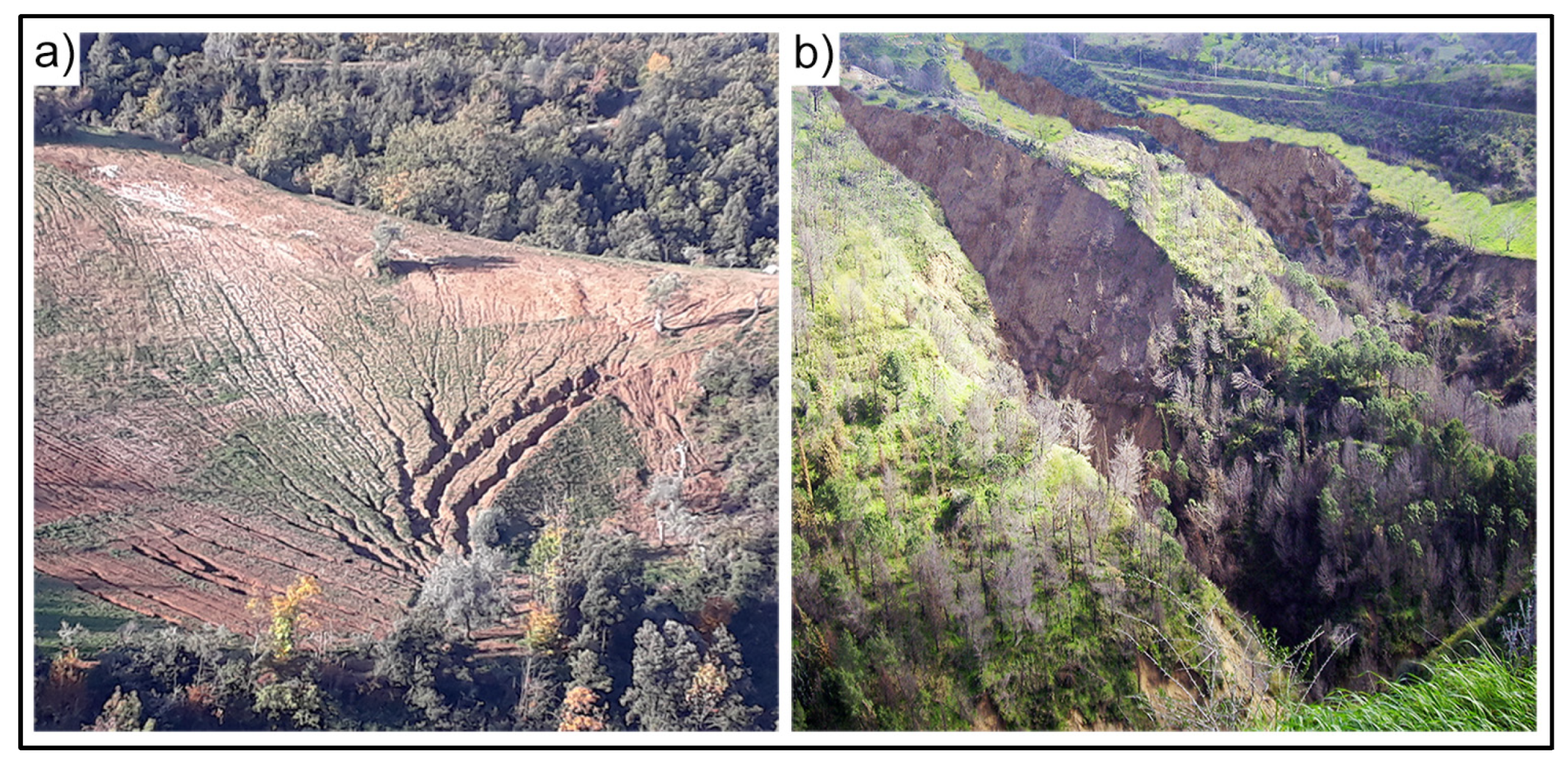
3.1. Gully Erosion Inventory

The inventory of the spatial distribution of gullies is fundamental data for mapping gully erosion susceptibility because it represents the dependent variable in the prediction models. In this work, the inventory map of gully erosion landforms was realised using the visual interpretation of orthophotos, dating 2008 (1:5000 scale) and downloaded by the website of the Cartographic Center of Calabria region (http://geoportale.regione.calabria.it/opendata, accessed on 30 November 2020), and Google Earth images available from 2010 to 2022. In addition, field investigations were carried out using a GPS receiver device to localise the gullies’ position. The field survey highlighted that gully erosion processes are mainly active in areas with sparse or no vegetation cover, as well as in arable lands and grasslands. Several ephemeral gullies were observed on croplands, mainly during intense rainfall events due to water runoff concentration. These processes cause a severe soil loss (Figure 2a). Permanent gullies with steep and bare walls, indicating an active stage of dissection, were mapped on hillslopes where sand and conglomerate deposits crop out (Figure 2b). In addition, a dense network of gullies often dissects clayey slopes. Within the catchment, a total of 529 areas involved in gully erosion processes were recognised. The gully areas were mapped in polygon format and, successively, each polygon was transformed to a point representing the centroid of the head-cut area of the gullies (Figure 1b).

3.2. Gully Erosion Predisposing Factors

Selecting predisposing factors is an important step for implementing a reliable gully erosion susceptibility model [20,22]. Numerous geo-environmental features, such as geology, soil, topography, hydrology, and land cover/use, control the gully’s occurrence [1,11,13,46]. However, no universal guideline exists regarding the predisposing factors that should be used in the gully erosion prediction models. Several studies employed different geo-environmental variables based on the availability, reliability, and practicality of the data [13,20,24,25,47,48]. In this study, the predisposing factors were rationally selected, considering the data availability, previous knowledge of the study area, and concerning the relevant literature [23,24,26,46]. Using this procedure, a set of 12 predisposing factors was selected, including lithology, soil texture, soil bulk density, land use, drainage density, slope gradient, aspect, length–slope (LS) factor, plan curvature, stream power index (SPI), topographic position index (TPI), and topographic wetness index (TWI).

The geological map of the Calabria region at scale 1:25,000 was used to create the lithology layer (Figure 3a). The data concerning the soil texture and soil bulk density (Figure 3b,c) were extracted from the digital soil map of Calabria (scale 1:250,000) [44]. Regarding the land use layer (Figure 3d), it was extracted from the Corine Land Cover map of Italy (scale 1:100,000), downloaded from the website of ISPRA (http://www.sinanet.isprambiente.it, accessed on 13 February 2021).

The drainage density map (Figure 3e), defined as the total length of the hydrographic network per unit area (1 km² in this study), was obtained by interpolating the hydrographic network using the line density tool implemented in ArcGIS 10.8 software. Instead, the topographic factors such as slope gradient, aspect, LS, plan curvature, SPI, TPI, and TWI (Figure 3f–l) were elaborated from a digital terrain model (DTM) with a spatial resolution of 5 × 5 m, using the software SAGA-GIS version 8.0.1 [49].

The data regarding the hydrographic network and DTM were downloaded from the website of the Cartographic Center of Calabria region (http://geoportale.regione.calabria.it/opendata, accessed on 10 March 2021).

For the analysis of gully erosion susceptibility, the thematic layers elaborated for each predisposing factor were transformed in raster layers with a pixel size of 5 m.

4. Methodology

The methodology applied in this study is based on five main steps: (i) spatial database construction; (ii) multi-collinearity analysis; (iii) implementing the maximum entropy (MaxEnt) method for mapping gully erosion susceptibility; (iv) assessing the accuracy and robustness of the MaxEnt method and related gully erosion susceptibility map; and (v) sensitivity analysis of predisposing factors. More details of the methodology used are explained below.

4.1. Multi-Collinearity Test

Before implementing the MaxEnt method, a multi-collinearity test was performed to determine the collinearity rate among the selected predisposing factors. Consequently, the highly correlated factors were removed to avoid bias in the susceptibility model [50]. The multi-collinearity can be defined as the linear correlation between two or more variables in a dataset [51]. In order to test the multi-collinearity between the 12 predisposing factors chosen for gully erosion susceptibility analysis, the variance inflation factor (VIF) and tolerance (TOL) index were calculated [52]. In general, values of VIF > 10 and TOL < 0.1 indicate collinearity problems between the variables [53]. In this study, multi-collinearity analysis was made by means of the IBM SPSS software, version 29.

4.2. Maximum Entropy Method

In this study, the MaxEnt method [54] was applied for modelling the potential and future distribution of gully erosion-prone areas based on a set of geo-environmental factors. MaxEnt is a machine learning method based on the entropy maximisation principle [55], which can handle data from various measurement scales without relying on parametric statistical assumptions. This method is based on information theory and statistics with the concept of the best approximation of an unknown probability distribution [56]. The MaxEnt approach was widely applied in research related to environmental and ecological modelling [54,55,57], landslide susceptibility [52,58,59,60], as well as gully erosion susceptibility [22,34,61,62].

Applying the MaxEnt method, based on the presence-only features, the gully erosion susceptibility is defined as the probability distribution within the study area. The probability of gully occurrences is calculated with the following [59]:

$$\mathrm{P}\left(\mathrm{y}=1|\mathrm{x}\right)=\frac{\mathrm{P}\left(\mathrm{y}=1)\mathrm{P}\mathrm{x}|\mathrm{y}=1\right)}{\mathrm{P}\left(\mathrm{x}\right)}=\frac{\mathrm{P}\left(\mathrm{y}=1\right)\mathsf{\pi }\left(\mathrm{x}\right)}{1/\left|\mathrm{x}\right|}$$

(1)

where P (y = 1) is the probability of occurrence of gullies and |x| is the number of gullies occurring in the study area; x denotes a random site over the study area. The π (x) required by the MaxEnt method is similar to the estimate of the Gibbs probability distribution function [63]. If n variables are assumed in the model (f_i, i = 1, 2,…, n), the Gibbs probability distribution can be written as follows:

$${\mathrm{q}}_{\mathsf{\lambda }}\left(\mathrm{x}\right)=\frac{\mathrm{e}\mathrm{x}\mathrm{p}({\sum }_{\mathrm{i}=1}^{\mathrm{n}}{\mathsf{\lambda }}_{\mathrm{i}}{\mathrm{f}}_{\mathrm{i}}\left(\mathrm{x}\right))}{{\mathrm{Z}}_{\mathsf{\lambda }}}$$

(2)

where Z_λ is the normalisation constant and λ is the sum of the vector weights assigned to the features. The MaxEnt method searches for the Gibbs distribution function that could maximise the log-likelihood of probability and minimise the estimation error. Supposing that m gully phenomena occurred in the study area, the difference between the log-likelihood calculation and regularisation is maximised using the formula of Phillips and Dudík [63]:

$$\frac{1}{\mathrm{m}}{\sum }_{\mathrm{i}=1}^{\mathrm{m}}1\mathrm{n}\left(\mathrm{q}\mathsf{\lambda }\left({\mathrm{X}}_1\right)\right)-{\sum }_{\mathrm{j}=\mathrm{i}}^{\mathrm{n}}{\mathsf{\beta }}_{\mathrm{j}}\left|{\mathsf{\lambda }}_{\mathrm{i}}\right|$$

(3)

where β_j is the normalised variable. In Equation (3), the first term is used for the maximum degree of fitting model value and the second is used for normalising the value. The MaxEnt method was applied using Maxent software, version 3.4.4. The probability of gully occurrence was set to 0.5, while the maximum number of iterations before interrupting the model building was set to 500. However, a convergence threshold was set to stop the training phase when the drop in log loss per iteration fell under a value of 0.00001. More details on the MaxEnt algorithm are given in Phillips et al. [54].

4.3. Implementing Gully Erosion Susceptibility Model

In this work, the k-fold cross-validation technique was applied to test the reliability of the MaxEnt method for mapping the gully erosion susceptibility. The k-fold cross-validation is a statistical validation approach largely used for evaluating predictive models in the field of geo-environmental sciences [26,64,65]. The prediction model is trained and validated k times, using a different fold as the testing set each time. Applying the k-fold cross-validation procedure was chosen to decrease the negative effects of a random selection of the training and testing sets on the model’s performance [64]. In the k-fold cross-validation, the dataset is uniformly and randomly divided into k folds (f₁, f₂, … f_k) of analogous size [65]. The advantage of this method is that all samples are used for training and testing the model [26]. Therefore, k − 1 folds are used for training the model, and the last fold is used for testing. The process is replicated k − 1 times so that each fold is considered for testing.

This research performed the k-fold cross-validation by randomly partitioning the gully erosion inventory (529 gully points) into 10 folds or subsets of approximately equal size (train-to-test ratio 90:10). Then, to calibrate the gully erosion susceptibility model, the MaxEnt algorithm was run 10 times (equal to the number of folds) to consider each subset for the training and testing phase. For each of the 10 built models, in turn, nine folds were used for the calibration phase, while one fold was used for testing the calibrated model.

For validating the predictive performance of each generated model, the goodness-of-fit (based on the training set) and prediction capability (based on the testing set) were determined by calculating the confusion matrix parameters (accuracy and kappa coefficient), the receiver operating characteristics (ROC) curve, and related area under curve (AUC) [66,67]. The confusion matrix consists of the following indexes: true positives (TP), true negatives (TN), false positives (FP), and false negatives (FN), where TP and TN are the pixels correctly classified, while FP and FN are the pixels incorrectly classified. These indexes allow the models’ overall accuracy to be determined, which is the number of pixels that the models correctly classified. The accuracy is calculated using the following equation:

$$\mathrm{A}\mathrm{c}\mathrm{c}\mathrm{u}\mathrm{r}\mathrm{a}\mathrm{c}\mathrm{y}=\frac{\mathrm{T}\mathrm{P}+\mathrm{T}\mathrm{N}}{\mathrm{T}\mathrm{P}+\mathrm{T}\mathrm{N}+\mathrm{F}\mathrm{P}+\mathrm{F}\mathrm{N}}$$

(4)

The kappa coefficient was determined using the components of the confusion matrix [68]. The kappa coefficient (K) assesses the consistency of the susceptibility model to classify correctly the pixels affected by gullies [20]. K was expressed as the ratio of the observed agreement beyond that occurring by chance and can be determined follows:

$$\mathrm{K}\mathrm{a}\mathrm{p}\mathrm{p}\mathrm{a}=\frac{{\mathrm{P}}_{\mathrm{o}\mathrm{b}\mathrm{s}}-{\mathrm{P}}_{\mathrm{e}\mathrm{x}\mathrm{p}}}{1-{\mathrm{P}}_{\mathrm{e}\mathrm{x}\mathrm{p}}}$$

(5)

where Pobs is the amount of pixels classified correctly as gullies or non-gullies and P_exp is the amount of pixels for which the agreement is expected by chance [68]. P_obs and P_exp were calculated as follows:

$${\mathrm{P}}_{\mathrm{o}\mathrm{b}\mathrm{s}}=\frac{\mathrm{T}\mathrm{P}+\mathrm{T}\mathrm{N}}{\mathrm{n}}$$

(6)

$${\mathrm{P}}_{\mathrm{e}\mathrm{x}\mathrm{p}}=\frac{\left(\mathrm{T}\mathrm{N}+\mathrm{F}\mathrm{P}\right)\times \left(\mathrm{T}\mathrm{N}+\mathrm{F}\mathrm{N}\right)+\left(\mathrm{F}\mathrm{N}+\mathrm{T}\mathrm{P}\right)\times (\mathrm{F}\mathrm{P}+\mathrm{T}\mathrm{P})}{\sqrt{\mathrm{N}}}$$

(7)

where n is the number of pixels classified correctly as gullies or not gullies and N is the total number of pixels. According to K values, the performance of the model can be classified as poor (0–0.2), fair (0.2–0.4), moderate (0.4–0.6), substantial (0.6–0.8), and almost perfect (0.8–1) [69].

The ROC curve is a bi-dimensional graph that displays, for different likelihood (susceptibility) threshold values, the TP rate (sensitivity) on the Y-axis and the FP rate (1-specificity) on the X-axis [66]. The sensitivity and specificity were calculated using the following equations:

$$\mathrm{S}\mathrm{e}\mathrm{n}\mathrm{s}\mathrm{i}\mathrm{t}\mathrm{i}\mathrm{v}\mathrm{i}\mathrm{t}\mathrm{y}=\frac{\mathrm{T}\mathrm{P}}{\mathrm{T}\mathrm{P}+\mathrm{F}\mathrm{N}}$$

(8)

$$\mathrm{S}\mathrm{p}\mathrm{e}\mathrm{c}\mathrm{i}\mathrm{f}\mathrm{i}\mathrm{c}\mathrm{i}\mathrm{t}\mathrm{y}=\frac{\mathrm{T}\mathrm{N}}{\mathrm{F}\mathrm{P}+\mathrm{T}\mathrm{N}}$$

(9)

The ROC curves were created both for the testing and training datasets to evaluate the models’ predictive performances and investigate their fit to the training observations. The AUC-ROC curve was calculated to quantify the effectiveness of the model [70]. The values of AUC can range from 0.5 (randomness) to 1 (perfect discrimination). The closer the value of AUC is to 1, the higher the model’s predictive capability [66,70]. According to Hosmer and Lemeshow [71], the predictive ability of a model based on the AUC value can be classified as follows: poor (0.5–0.6), moderate (0.6–0.7), good (0.7–0.8), very good (0.8–0.9), and excellent (0.9–1).

Additionally, to reveal the overall predictive ability and robustness (i.e., model response when the training and testing set change) of the MaxEnt method, the mean and standard deviation were computed for each performance parameter.

Using a GIS-based spatial analysis, implemented in ArcGIS software, the maps of probability of gully spatial occurrence, provided by 10 calibration models, were averaged to yield a single gully erosion susceptibility map. This susceptibility map, characterised by values of probability in each pixel that vary from 0 to 1, was categorised into five classes using the equal interval method (0.0 to 0.2, 0.2 to 0.4, 0.4 to 0.6, 0.6 to 0.8, and 0.8 to 1.0). These classes were defined, from 0 to 1, as follows: very low, low, moderate, high, and very high.

In addition, for assessing the consistency of the susceptibility classes, the index of relative gully erosion density (R) method was employed [72]. The R index was calculated using Equation (10).

$$\mathrm{R}=\frac{({\mathrm{x}}_{\mathrm{i}}/{\mathrm{X}}_{\mathrm{i}})}{\sum {\mathrm{x}}_{\mathrm{i}}/{\mathrm{X}}_{\mathrm{i}}}\times 100$$

(10)

where x_i is the percentage of gullies for each susceptibility class and X_i is the percentage of pixels of each susceptibility class. If the values of the R index are higher in the very high and high susceptibility classes, the efficiency of the map can be defined as good.

Finally, exploiting the 10 replicate calibration models, the standard deviation for the probability estimates of each pixel was also computed, allowing the uncertainty in model prediction to be evaluated quantitatively. The standard deviation is a good indicator of model stability [73,74]. Specifically, a narrow standard deviation indicates lower uncertainty, suggesting that several model iterations do not bias the accuracy.

4.4. Detecting Predisposing Factors’ Sensitivity

The sensitivity of predisposing factors was analysed through the jackknife test [24,58,59,75]. In model calibration phase, the sensitivity analysis plays an important role because it allows identification of the percentage of the relative importance (PRI) of each predisposing factor for modelling gully erosion susceptibility [58,59,75,76]. In the jackknife test, the importance of a predisposing factor is estimated by excluding, in turn, each one in the constructed model and using the remaining factors. Each model’s performance was executed by computing the AUC value [58,75]. The following equation was applied to compute each predisposing factor’s PRI [76]:

$$\mathrm{P}\mathrm{R}\mathrm{I}=\frac{({\mathrm{A}\mathrm{U}\mathrm{C}}_{\mathrm{a}\mathrm{l}\mathrm{l}}-{\mathrm{A}\mathrm{U}\mathrm{C}}_{\mathrm{i}})}{{\mathrm{A}\mathrm{U}\mathrm{C}}_{\mathrm{a}\mathrm{l}\mathrm{l}}}\times 100$$

(11)

where AUC_all is the value of AUC computed from the prediction model using all predisposing factors, while AUC_i represents the AUC value of the factor excluded from the computation of the model. Therefore, high values of PRI highlight a more significant influence of the predisposing factor in the model [75].

5. Results

5.1. Multi-Collinearity Analysis

The multi-collinearity test was applied to check the relationship between the geo-environmental variables selected for gullies’ susceptibility analysis.

Table 1. Multi-collinearity results among the predisposing factors selected for modelling gully erosion susceptibility.

Predisposing Factors	Multi-Collinearity
	VIF	TOL
Lithology	1.66	0.60
Soil texture	1.56	0.64
Soil bulk density	2.07	0.48
Land use	1.78	0.57
Drainage density	2.10	0.48
Slope gradient	2.96	0.34
Slope aspect	1.34	0.74
LS factor	3.10	0.32
Plan curvature	1.52	0.66
SPI factor	1.96	0.51
TPI factor	2.18	0.46
TWI factor	1.58	0.63

shows the results of the test carried out through VIF and TOL estimation and its comparison with predefined critical values (VIF > 10 and TOL < 0.1). The highest and lowest values of VIF are 3.10 and 1.34, respectively; whereas, regarding the TOL index, the highest value is 0.74 and the lowest is 0.32. This indicates that no predisposing factors exceed the threshold values and, consequently, there is no problem of multi-collinearity between the 12 predisposing factors chosen for implementing the susceptibility model.

5.2. Modelling Gully Erosion Susceptibility

This study employed the MaxEnt method for modelling the gully erosion susceptibility within the Mesima catchment (southern Italy). To implement the susceptibility model, 12 predisposing factors (lithology, soil texture, soil bulk density, land use, drainage density, slope gradient, slope aspect, plan curvature, LS, SPI, TPI, and TWI) and a gully’s inventory were used as input variables. Additionally, a 10-fold cross-validation approach was applied to test the predictive capability and stability (robustness) of the MaxEnt algorithm. The dataset was split into ten folds, nine of which were used for the calibration and one for the validation.

The findings of the MaxEnt algorithm performance for the calibration and validation phases are summarised in

Table 2. Predictive performance of calibration and validation phases based on 10-fold cross-validation of the gully erosion susceptibility model.

Fold Numbers	Calibration			Validation
	Accuracy	Kappa Coeff.	AUC	Accuracy	Kappa Coeff.	AUC
1	0.923	0.846	0.946	0.902	0.804	0.924
2	0.932	0.864	0.954	0.912	0.824	0.948
3	0.935	0.870	0.956	0.911	0.822	0.949
4	0.936	0.872	0.964	0.920	0.841	0.952
5	0.946	0.893	0.969	0.916	0.832	0.952
6	0.955	0.910	0.975	0.921	0.843	0.963
7	0.954	0.908	0.977	0.953	0.907	0.975
8	0.938	0.876	0.969	0.916	0.833	0.954
9	0.944	0.888	0.972	0.941	0.882	0.967
10	0.921	0.843	0.953	0.921	0.843	0.937
Min	0.921	0.843	0.946	0.902	0.804	0.924
Max	0.955	0.910	0.977	0.953	0.907	0.975
Mean	0.938	0.877	0.964	0.921	0.843	0.952
St.dev.	0.012	0.023	0.011	0.015	0.030	0.015

. The results presented in Table 2 allowed performance results obtained by each one of the 10-fold cross-validation to be compared. Concerning the calibration phase, the results of the performance metrics, i.e., accuracy, kappa coefficient, and AUC, always have excellent goodness fit of the prediction model, with a mean value of kappa coefficient and AUC of 0.877 and 0.964, respectively. As for the validation phase, the results showed a similar ranking pattern to the calibration phase (Table 2) and, consequently, the susceptibility model displayed excellent predictive skill (mean AUC = 0.952). In addition, the low values of standard deviation, obtained for all three performance parameters (Table 2), showed that the effects of different calibration and validation sets on the MaxEnt method accuracy are not significant, highlighting a strong stability (robustness) of the susceptibility model.

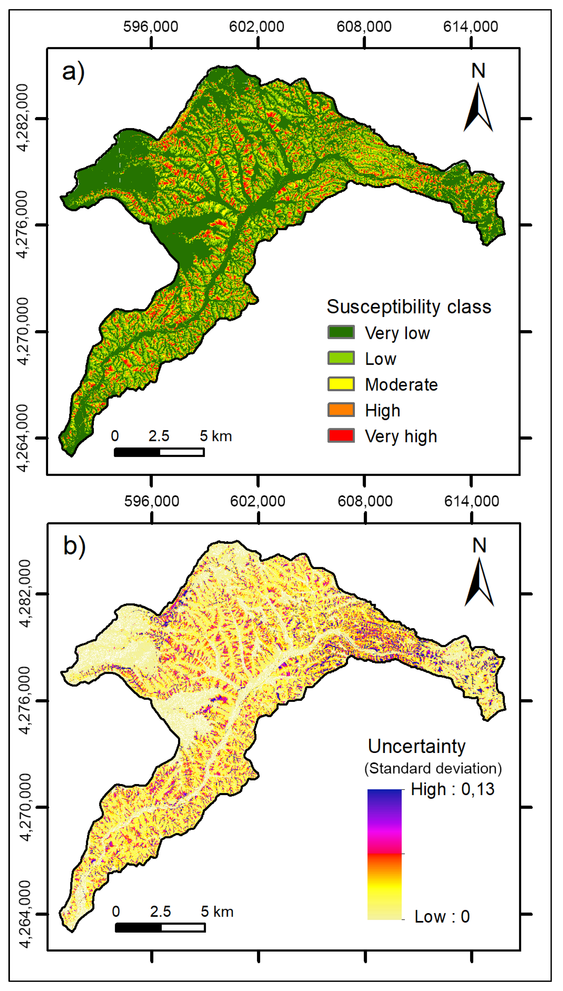
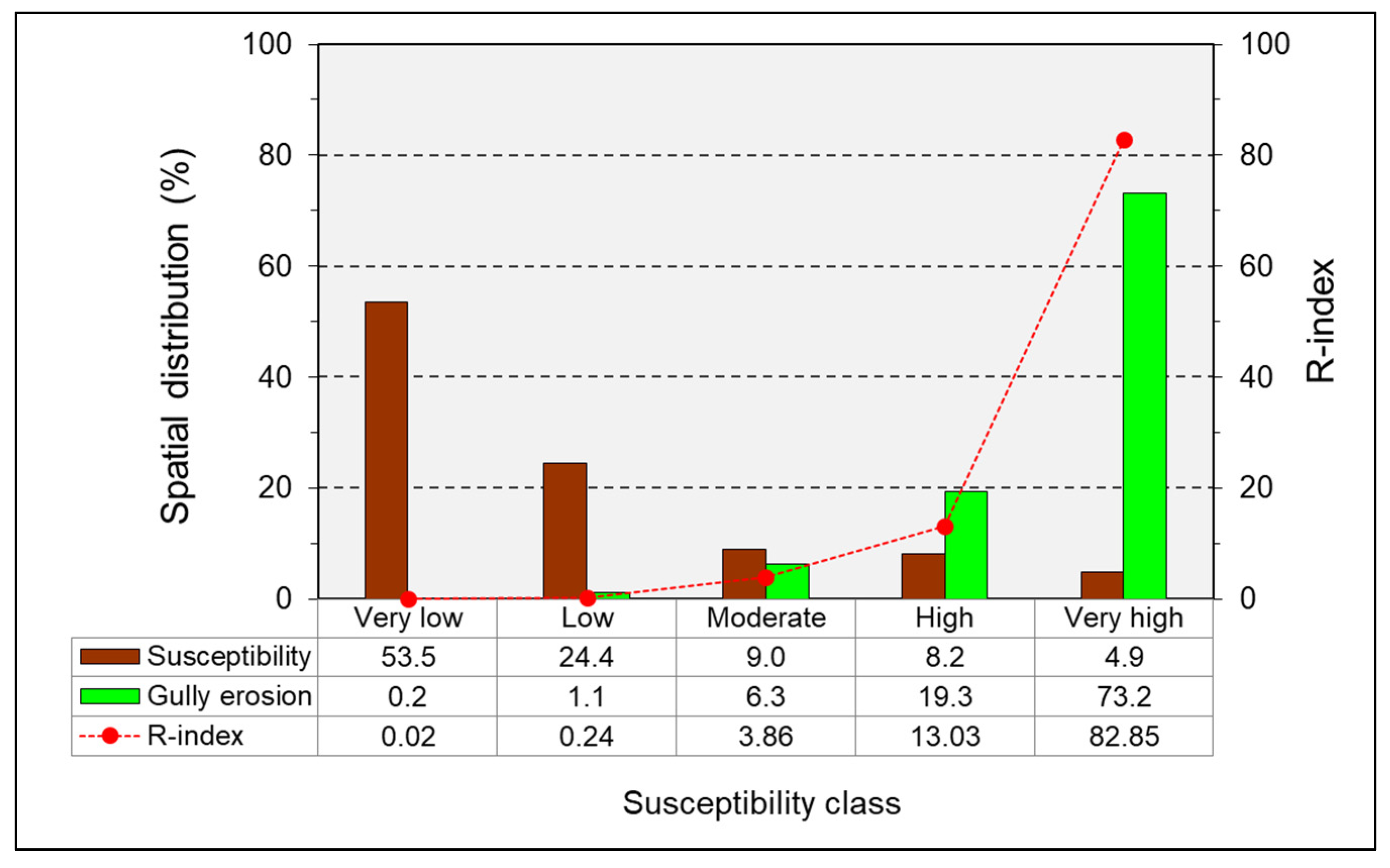
5.3. Gully Erosion Susceptibility Map

A gully erosion susceptibility map of the Mesima stream catchment was produced (Figure 4a) after assessing the prediction performance of the MaxEnt method. The susceptibility map was obtained by averaging 10 probability estimates using a 10-fold cross-validation analysis. The map indicates the probability of gully erosion occurrence at each point of the study area.

The susceptibility values range between 0.01 and 1, with a mean value of 0.257 and a standard deviation of 0.01. The pixels with susceptibility values closer to 1 indicate a high probability of gully occurrence, whereas a low probability happens with values closer to 0. In the map in Figure 4a, we have classified the gully erosion susceptibility values into five classes based on the equal interval method as follows: very low, low, moderate, high, and very high. The areal distribution of the recognised classes is shown in Figure 5. Most of the areas in the catchment fell in the low and very low susceptibility classes (about 78% of the total area); instead, the areas affected by very high and high susceptibility were generally fewer (13.1%).

The comparison between the susceptibility map and gully erosion inventory allowed the gullies’ spatial distribution in the five susceptibility classes to be verified (Figure 5). The achieved result showed that the susceptibility map displayed a remarkable agreement with the gully inventory. Indeed, about 92.5% of gullies were correctly classified, falling in the areas mapped as having high and very high susceptibility (probability values between 0.6 and 1). Furthermore, less than 1.2% of the recognised gullies fall in the low and very low susceptibility classes (Figure 5). Hence, the susceptibility map highlights a high reliability for detecting gully-prone areas.

In addition, the validity of the gully erosion susceptibility map was confirmed also by the computation of the R-index (Figure 5). In particular, the R-index values increase from very low to very high susceptibility classes, remarking that the susceptibility map is in agreement with the spatial occurrence of gullies.

The spatial pattern of the uncertainty associated with the obtained susceptibility map was produced by computing the standard deviation of the 10 estimates of probability gully occurrence (Figure 4b). The uncertainty (standard deviation) values range from 0 to 0.13 (mean value equal to 0.003), which reveal small variation among the 10 estimates of probability and, consequently, they show a high robustness of the prediction model. The inspection of the map (Figure 4b) shows that the lowest values of uncertainty were mainly measured for areas with very low susceptibility (probability ≤ 0.20) and, subordinately, in zones mapped as highly susceptible (probability ≥ 0.80). These results show that the prediction models allowed the no-prone areas to be rightly identified from those prone to gully erosion occurrence. Conversely, the areas of the catchment with moderate susceptibility show the highest uncertainty, indicating that the susceptibility model is less reliable in these areas [73,74].

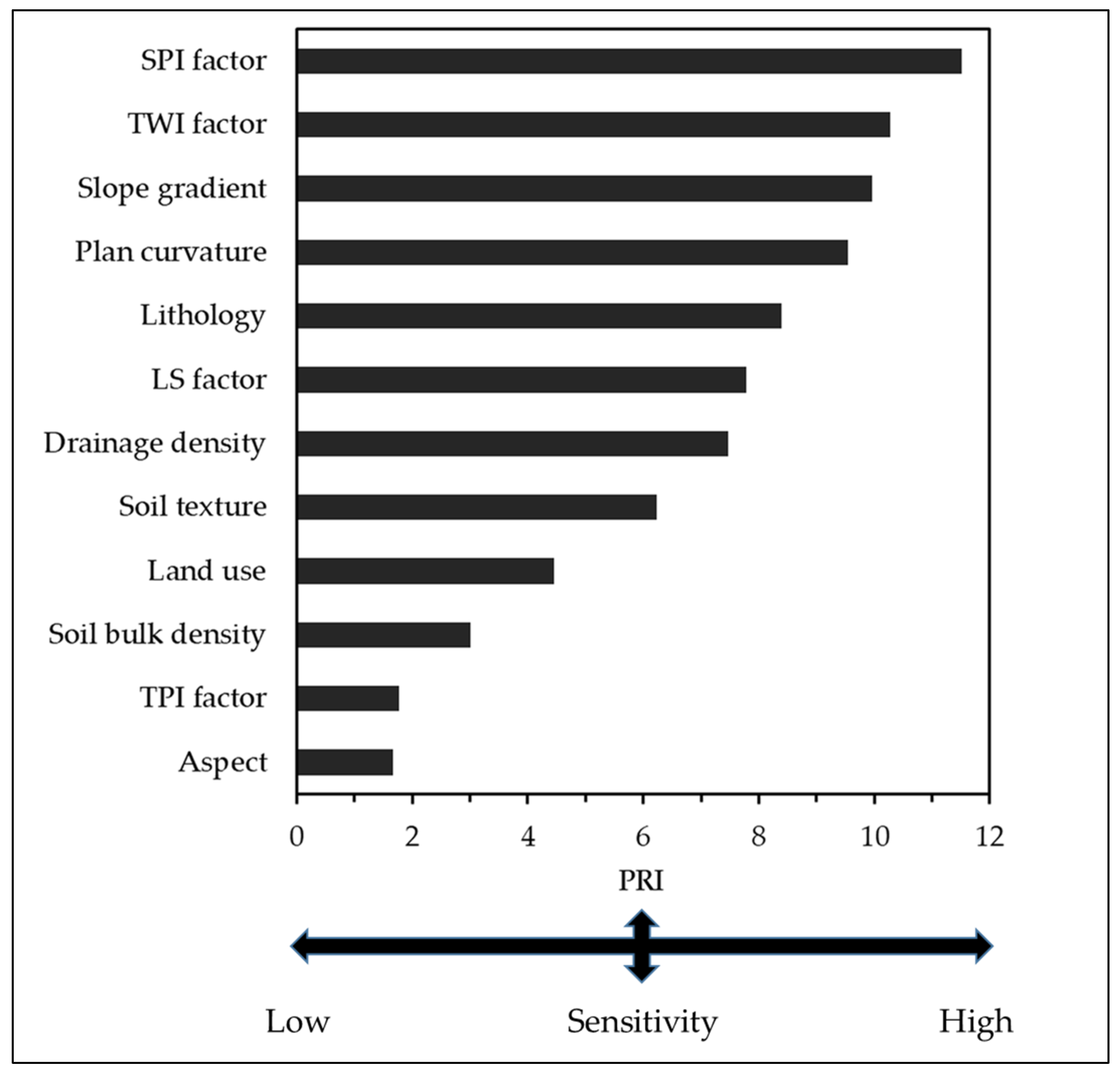
5.4. Sensitivity Analysis of Predisposing Factors

The relative importance of each predisposing factor used for modelling gully erosion susceptibility was examined based on the jackknife test and related PRI index. The output results, summarised in Figure 6, show that all the predisposing factors contributed positively to constructing the gully erosion susceptibility model. This outcome denotes a correct selection of the geo-environmental variables used in the susceptibility analysis. However, the predisposing factors with the greatest sensitivity were SPI (PRI = 11.51), TWI (PRI = 10.27), slope gradient (PRI = 9.96), and plan curvature (PRI = 9.54); instead, minimal sensitivity was observed in soil bulk density (PRI = 3.05), TPI (PRI = 1.76) and aspect (PRI = 1.66) (Figure 6).

Overall, the sensitivity analysis highlighted that the importance of topographical factors was relatively higher than the other predisposing factors used in this study.

6. Discussion

A complex interaction of several geo-environmental variables drives the spatial pattern of gully erosion [1,24,33,77]. Consequently, understanding the cause-and-effect of these geomorphic processes and accurately mapping the areas prone to gully erosion can provide valuable insights for identifying appropriate management strategies for a territory [78]. Various statistical and machine learning methods have been applied in the last decade to model and map gully erosion susceptibility [13,21,22,23,29,31,32,79]. However, no agreement has yet been made on selecting the best model for predicting gully erosion occurrence. This lack of consensus is because the formation of gullies is influenced by the specific topographical, geomorphological, geological, pedological, and hydrological settings in each study area [2,24,31,46,80]. Several scientific papers have asserted that machine learning techniques generally perform better than traditional statistical methods [19,26,29,32,61]. In this study, we tested the predictive capabilities of the MaxEnt method for mapping the gully erosion susceptibility in a catchment of the Calabria region (South Italy). To implement the MaxEnt algorithm, 12 predisposing factors, such as: lithology, soil texture, soil bulk density, land use, drainage density, slope gradient, slope aspect, plan curvature, LS, TPI, SPI, and TWI, were selected based on the previous scientific literature and detailed surveys in the study area [13,24,26,29,31,36,42,61]. Using a multi-collinearity diagnosis, the interdependence or redundancy between the mentioned factors was analysed [81]. The results showed no multi-collinearity among the 12 factors used to build the susceptibility model.

The predictive capability of the trained model, using the 10-fold cross-validation, was evaluated using confusion matrix measures and the AUC-ROC curve. According to the results presented in Table 2, the accuracy measures for all models are very similar in each fold. The model’s excellent goodness-of-fit and predictive skill (AUC values well above 0.90) demonstrate the reliability of the method applied and confirm that accurate predictions of gullies’ occurrence may be obtained from implementing the MaxEnt method. In addition, the high accuracy of the prediction model also demonstrates the validity of the gully erosion inventory and the geo-environmental variables selected as predisposing factors. Therefore, tiny differences in the predictive capacities were observed during the 10-fold cross-validation, which suggests that the MaxEnt method is able to produce a reliable and robust gully erosion predictive model when changing the calibration and validation sets. Moreover, the very low values of standard deviation obtained for accuracy, kappa coefficient, and AUC (Table 2) confirmed a certain stability of the prediction model. This suggests that the MaxEnt method is particularly promising for mapping the complex spatial pattern of gully erosion-prone areas [52]. The findings also highlight that the 10-fold cross-validation approach is adequate to reduce the negative effects of random sampling on the performance of the machine learning method [81]. Furthermore, the k-fold cross-validation technique can improve the predictive capability of the gully erosion susceptibility model because it helps to generate new accuracy measures and grow the robustness of other conventional ones.

The achieved findings agree with those shown in previous studies, which applied the MaxEnt algorithm to assessing gully erosion susceptibility in different geological contexts [21,26,29,47,52,61,82]. Compared to other machine learning methods frequently used to evaluate the susceptibility of gully erosion, such as random forest [20,25,83], support vector machine [33,84], boosted regression tree [21,22], and artificial neural network [22,33,85], the MaxEnt method has the advantage of not requiring a dataset of points corresponding to areas without gullies to use as a dependent variable to run the model. In this case, all areas outside the gully landforms are considered as “no-gully” but the current absence of gullies does not necessarily mean that, in these areas, there is no likelihood that gullies might develop in the future. Additionally, this method can manage and use large datasets and can recognise and consider the nonlinear relationship between independent variables and dependent variables [58,59]. The MaxEnt method maximises the likelihood of the calibration dataset to calculate the weights of predisposing factors selected for building the prediction model [60,86].

As previously discussed, the final susceptibility map was produced by averaging the probability estimates computed by the 10 iterations (folds) of the MaxEnt method. Thus, this map shows the probability of gully occurrence for each pixel of the study area. The probability values, ranging from 0 to 1, were classified into five levels (very high, high, moderate, low, and very low). The susceptibility map reveals a very heterogeneous spatial distribution due to the several geo-environmental factors affecting gully erosion processes. The areal distribution of the different susceptibility levels shows a decreasing trend from very low to very high classes of susceptibility (Figure 5); therefore, most portions of the study area fall in zones with low susceptibility values and only a very small area shows a higher susceptibility level. High and very high susceptibility classes are mainly located along the upstream catchment (Figure 4a) and accounted for 8.2% and 4.9% of the total area, respectively. In these zones, the highest susceptibility values were found in cultivated areas or areas covered by sparse scrub and/or herbaceous vegetation, characterised by steep clayey slopes with a concave morphology. The high probability of gully formation in cultivated fields can be related to improper cultivation practices [13,14,18,46]. In contrast, the lowest levels of susceptibility were recorded in the downstream catchment, where alluvial deposits crop out and a flat morphology characterises the landscape. Moreover, low susceptibility classes were detected in forest areas, where water erosion processes are generally minimal because the dense aboveground biomass dissipates the raindrop energy.

In agreement with Merghadi et al. [87], these results show that the susceptibility map is reliable because it classified a significant portion of the study area as low and very low susceptibility (about 80%). In contrast, the highest susceptibility classes include only small zones of the catchment (Figure 4a). Moreover, the goodness of the susceptibility map was also confirmed by the elevated presence of the gully landforms (92.5%) in high and very high susceptibility classes. Thus, this map can correctly identify the spatial distribution of ephemeral and permanent gullies and suggests those areas that are actually not affected by gully erosion phenomena but have a high predisposition to developing gully processes in the future [13,52]. Furthermore, the outcomes achieved by the R-index calculation testify to the consistency of the gully erosion susceptibility map [72]. Indeed, high R-index values were collected in high and very high susceptibility classes, which cover only a small percentage of the study area. In contrast, the R-index values decrease for the low and very low classes, showing a poor occurrence of gully erosion (Figure 5).

Furthermore, we analysed the uncertainty of the susceptibility map by determining the standard deviation of the probability estimates computed using the 10-fold cross-validation. The standard deviation of gully occurrence probability measures the prediction model uncertainty associated with several susceptibility estimates [88]. A higher standard deviation value indicates higher uncertainty (high variability of the susceptibility values between the different estimates), while lower values indicate better prediction results. The achieved results showed that the effects of the different calibration/validation sets on the predictive capability of the prediction model are insignificant because they exhibit slight variations in the standard deviation values. Consequently, the susceptibility map showed low uncertainty values for each map pixel (Figure 4b). Overall, these findings corroborated the good quality of the dataset used in the susceptibility analysis and the robustness of the method applied [73,86].

The susceptibility model allowed the assessment of the sensitivity of each predisposing factor providing valuable information for knowledge improving the spatial distribution of gully erosion. Therefore, in the current study, we evaluated the influence of the selected predisposing factors by calculating the PRI index. The outcomes showed that topographic factors like SPI, TWI, slope gradient, plan curvature, and LS mainly controlled the spatial pattern of gully erosion. The high influence of these factors on the susceptibility model agrees with previous studies affirming that the slope gradient, SPI, and LS show a high relation with gully development [46,47,80]. Indeed, these factors affect the runoff processes and consequently control the linear erosion intensity along the slopes [2,45,89]. For example, a high LS value increases the runoff velocity and, thus, raises the probability of gully erosion formation [90]. In this regard, several researchers in southern Italy identified topographic variables as the main factors in the occurrence of gully erosion [13,91,92]. Additionally, the results of the PRI model corroborate that other predisposing factors, such as lithology and drainage density, significantly impact the occurrence and further gully development in the study area (Figure 6). The lithological features in combination with soil texture distribution control the water infiltration rate and consequently influence gully formation and its evolution [45,93].

During field investigations, it was observed that, in several cases, the gully landforms fall within the first- or second-order drainage network because concentrated runoff promotes the gully erosion formation [13,32], whereas factors such as soil bulk density, TPI, and aspect do not contribute much to the susceptibility model (Figure 6).

The goals obtained in this study highlighted that applying the MaxEnt method can provide a very good assessment of the spatial pattern of gully erosion-prone areas and identify zones that need urgent interventions for mitigating the gully erosion risk. In addition, the method could be used for mapping gully erosion susceptibility in other areas of the Calabria region, particularly where similar geological and topographical features prevail.

Finally, although this study shows satisfactory results, future research is recommended to enhance gully erosion susceptibility mapping using site-specific variables, such as soil types, geotechnical parameters of the soil, and rainfall characteristics, which are not included in this study. In addition, possible future developments may involve analyses of the uncertainty of the input data, in combination with the detection of the raster resolution effect on prediction models.

7. Conclusions

This study aims to test the reliability of the MaxEnt machine learning method for mapping the gully erosion susceptibility and to detect the most important geo-environmental factors for the analysis of the erosion susceptibility in a catchment of the Calabria region (South Italy). Twelve predisposing factors were used to build the susceptibility model, including lithology, soil texture, soil bulk density, land use, drainage density, slope gradient, slope aspect, plan curvature, LS, SPI, TPI, and TWI and a gully inventory map.

The method’s predictive capability (goodness-of-fit and prediction skill) was tested by 10-fold cross-validation based on accuracy, kappa coefficient, and AUC parameters. On the basis of the obtained results, the MaxEnt method clearly demonstrated its ability to model gully erosion susceptibility, predicting the areas prone to gullies with excellent performance, as demonstrated by the high values of accuracy (>0.90), of the kappa coefficient (>0.80), and AUC (>0.92). Moreover, the results of the 10 iterations of the MaxEnt algorithm allowed the prediction model to be defined as very stable (robust) and with a low level of uncertainty.

The probability estimates’ mean value and standard were computed for each pixel of the study area by exploiting the 10-fold cross-validation. This procedure allowed the production of gully erosion susceptibility and uncertainty maps. The results showed small variations in the standard deviation values and, consequently, the susceptibility map denotes low levels of uncertainty for each pixel of the map.

The susceptibility map was classified into five classes: very low, low, moderate, high, and very high susceptibility, showing that high and very high susceptibility classes involved 13.1% of the total area. An excellent spatial agreement between the susceptibility and gully distribution classes was obtained by overlaying the susceptibility and gully erosion inventory maps. Indeed, in this procedure, 92.5% of the gullies were correctly classified, falling into high and very high susceptibility classes.

The outcomes also revealed that the selection and sensitivity analysis of the predisposing factors represent a key phase for reliable modelling of gully erosion susceptibility. Furthermore, all used predisposing factors showed significant importance on the prediction model’s performance, as testified by PRI index evaluation results. The predisposing factors that contributed more to the realisation of the gully erosion susceptibility model were SPI, TWI, slope gradient, plan curvature, LS, and lithology.

Finally, the high predictive capacity of the susceptibility model confirms that the MaxEnt method is able to produce accurate and robust gully erosion susceptibility maps. These maps may provide a valuable tool for local administrators to identify the most susceptible areas to gully erosion that need urgent interventions to mitigate the soil erosion risk.

References

1. Valentin, C.; Poesen, J.; Li, Y. Gully erosion: Impacts, factors and control. Catena 2005, 63, 132–153. [Google Scholar] [CrossRef]
2. Kakembo, V.; Xanga, W.W.; Rowntree, K. Topographic thresholds in gully development on the hillslopes of communal areas in Ngqushwa Local Municipality, Eastern Cape, South Africa. Geomorphology 2009, 110, 188–194. [Google Scholar] [CrossRef]
3. Vanmaercke, M.; Panagos, P.; Vanwalleghem, T.; Hayas, A.; Foerster, S.; Borrelli, P.; Rossi, M.; Torri, D.; Casali, J.; Borselli, L.; et al. Measuring, modelling and managing gully erosion at large scales: A state of the art. Earth Sci. Rev. 2021, 218, 103637. [Google Scholar] [CrossRef]
4. Haddadchi, A.; Nosrati, K.; Ahmadi, F. Differences between the source contribution of bed material and suspended sediments in a mountainous agricultural catchment of western Iran. Catena 2014, 116, 105–113. [Google Scholar] [CrossRef]
5. Chen, H.; Liu, G.; Zhang, X.C.; Shi, H.Q.; Li, H.R. Quantifying sediment source contributions in an agricultural catchment with ephemeral and classic gullies using 137Cs technique. Geoderma 2021, 398, 115112. [Google Scholar] [CrossRef]
6. Farias Amorim, F.; da Silva, Y.J.A.B.; Cabral Nascimento, R.; da Silva, Y.J.A.B.; Tiecher, T.; do Nascimento, C.W.A.; Gomes Minella, J.P.; Zhang, Y.; Ram Upadhayay, H.; Pulley, S.; et al. Sediment source apportionment using optical property composite signatures in a rural catchment, Brazil. Catena 2021, 202, 105208. [Google Scholar] [CrossRef]
7. Lal, R. Soil degradation by erosion. Land Degrad. Dev. 2001, 12, 519–539. [Google Scholar] [CrossRef]
8. Poesen, J.; Nachtergaele, J.; Verstraeten, G.; Valentin, C. Gully erosion and environmental change: Importance and research needs. Catena 2003, 50, 91–133. [Google Scholar] [CrossRef]
9. Amundson, R.; Berhe, A.A.; Hopmans, J.W.; Olson, C.; Sztein, A.E.; Sparks, D.L. Soil and human security in the 21st century. Science 2015, 348, 1261071. [Google Scholar] [CrossRef]
10. Borrelli, P.; Poesen, J.; Vanmaercke, M.; Ballabio, C.; Hervàs, J.; Maerker, M.; Scarpa, S.; Panagos, P. Monitoring gully erosion in the European Union: A novel approach based on the Land Use/Cover Area frame survey (LUCAS). Int. Soil Water Conserv. Res. 2022, 10, 17–28. [Google Scholar] [CrossRef]
11. Vandekerckhove, L.; Poesen, J.; Oostwoudwijdenes, D.J.; Gyssels, G.; Beuselinck, L.; De Luna, E. Characteristics and controlling factors of bank gullies in two semiarid Mediterranean environments. Geomorphology 2000, 33, 37–58. [Google Scholar] [CrossRef]
12. Conforti, M.; Pascale, S.; Pepe, M.; Sdao, F.; Sole, A. Denudation processes and landforms map of the Camastra River catchment (Basilicata—South Italy). J. Maps 2013, 9, 444–445. [Google Scholar] [CrossRef]
13. Conoscenti, C.; Angileri, S.; Cappadonia, C.; Rotigliano, E.; Agnesi, V.; Märker, M. Geomorphology Gully erosion susceptibility assessment by means of GIS-based logistic regression: A case of Sicily (Italy). Geomorphology 2014, 204, 399–411. [Google Scholar] [CrossRef]
14. Deng, Q.; Qin, F.; Zhang, B.; Wang, H.; Luo, M.; Shu, C.; Liu, H.; Liu, G. Characterizing the morphology of gully cross-sections based on PCA: A case of Yuanmou Dry-Hot Valley. Geomorphology 2015, 228, 703–713. [Google Scholar] [CrossRef]
15. Borrelli, L.; Conforti, M.; Mercuri, M. Lidar and UAV system data to analyse recent morphological changes of a small drainage basin. ISPRS Int. J. Geoinf. 2019, 8, 536. [Google Scholar] [CrossRef]
16. Pulice, I.; Scarciglia, F.; Leonardi, L.; Robustelli, G.; Conforti, M.; Cuscino, M.; Lupiano, V.; Critelli, S. Studio Multidisciplinare di Forme e Processi Denudazionali nell’area di Vrica (Calabria Orientale). Mem. Soc. Geogr. Italy 2009, 87, 403–417. [Google Scholar]
17. Terranova, O.; Antronico, L.; Coscarelli, R.; Iaquinta, P. Soil erosion risk scenarios in the Mediterranean environment using RUSLE and GIS: An application model for Calabria (Southern Italy). Geomorphology 2009, 112, 228–245. [Google Scholar] [CrossRef]
18. Conforti, M.; Buttafuoco, G.; Rago, V.; Aucelli, P.P.C.; Robustelli, G.; Scarciglia, F. Soil loss assessment in the Turbolo catchment (Calabria, Italy). J. Maps 2016, 12, 815–825. [Google Scholar] [CrossRef]
19. Amare, S.; Langendoen, E.; Keesstra, S.; Ploeg, M.V.D.; Gelagay, H.; Lemma, H.; Van Der Zee, S.E. Susceptibility to gully erosion: Applying random forest (RF) and frequency ratio (FR) approaches to a small catchment in Ethiopia. Water 2021, 13, 216. [Google Scholar] [CrossRef]
20. Rahmati, O.; Tahmasebipour, N.; Haghizadeh, A.; Pourghasemi, H.R.; Feizizadeh, B. Evaluating the influence of geo-environmental factors on gully erosion in a semi-arid region of Iran: An integrated framework. Sci. Total Environ. 2017, 579, 913–927. [Google Scholar] [CrossRef]
21. Arabameri, A.; Pradhan, B.; Pourghasemi, H.R.; Rezaei, K.; Kerle, N. Spatial modelling of gully erosion using GIS and R programing: A comparison among three data mining algorithms. Appl. Sci. 2018, 8, 1369. [Google Scholar] [CrossRef]
22. Garosi, Y.; Sheklabadi, M.; Pourghasemi, H.R.; Besalatpour, A.A.; Conoscenti, C.; Van Oost, K. Comparison of differences in resolution and sources of controlling factors for gully erosion susceptibility mapping. Geoderma 2018, 330, 65–78. [Google Scholar] [CrossRef]
23. Lana, J.C.; Castro, P.D.T.A.; Lana, C.E. Assessing gully erosion susceptibility and its conditioning factors in southeastern Brazil using machine learning algorithms and bivariate statistical methods: A regional approach. Geomorphology 2022, 402, 108159. [Google Scholar] [CrossRef]
24. Rahmati, O.; Kalantari, Z.; Ferreira, C.S.; Chen, W.; Soleimanpou, S.M.; Kapović-Solomun, M.; Seifollahi-Aghmiuni, S.; Ghajarnia, N.; Kazemabady, N.K. Contribution of physical and anthropogenic factors to gully erosion initiation. Catena 2022, 210, 105925. [Google Scholar] [CrossRef]
25. Bouramtane, T.; Hilal, H.; Rezende-Filho, A.T.; Bouramtane, K.; Barbiero, L.; Abraham, S.; Valles, V.; Kacimi, I.; Sanhaji, H.; Torres-Rondon, L.; et al. Mapping gully erosion variability and susceptibility using remote sensing, multivariate statistical analysis, and machine learning in South Mato Grosso, Brazil. Geosciences 2022, 12, 235. [Google Scholar] [CrossRef]
26. Garosi, Y.; Sheklabadi, M.; Conoscenti, C.; Pourghasemi, H.R.; Van Oost, K. Assessing the performance of GIS- based machine learning models with different accuracy measures for determining susceptibility to gully erosion. Sci. Total Environ. 2019, 664, 1117–1132. [Google Scholar] [CrossRef] [PubMed]
27. Rahmati, O.; Haghizadeh, A.; Pourghasemi, H.R.; Noormohamadi, F. Gully erosion susceptibility mapping: The role of GIS-based bivariate statistical models and their comparison. Nat. Hazards 2016, 82, 1231–1258. [Google Scholar] [CrossRef]
28. Al-Abadi, A.M.; Al-Ali, A.K. Susceptibility mapping of gully erosion using GIS-based statistical bivariate models: A case study from Ali Al-Gharbi District, Maysan Governorate, southern Iraq. Environ. Earth Sci. 2018, 77, 249. [Google Scholar] [CrossRef]
29. Azareh, A.; Rahmati, O.; Rafiei-Sardooi, E.; Sankey, J.B.; Lee, S.; Shahabi, H.; Ahmad, B. Bin Modelling gully-erosion susceptibility in a semi-arid region, Iran: Investigation of applicability of certainty factor and maximum entropy models. Sci. Total Environ. 2019, 655, 684–696. [Google Scholar] [CrossRef]
30. Dube, F.; Nhapi, I.; Murwira, A.; Gumindoga, W.; Goldin, J.; Mashauri, D.A. Potential of weight of evidence modelling for gully erosion hazard assessment in Mbire District–Zimbabwe. Phys. Chem. Earth 2014, 67–69, 145–152. [Google Scholar] [CrossRef]
31. Arabameri, A.; Pradhan, B.; Rezaei, K. Gully erosion zonation mapping using integrated geographically weighted regression with certainty factor and random forest models in GIS. J. Environ. Manag. 2019, 232, 928–942. [Google Scholar] [CrossRef] [PubMed]
32. Arabameri, A.; Yamani, M.; Pradhan, B.; Melesse, A.; Shirani, K.; Tien Bui, D. Novel ensembles of COPRAS multi-criteria decision-making with logistic regression, boosted regression tree, and random forest for spatial prediction of gully erosion susceptibility. Sci. Total Environ. 2019, 688, 903–916. [Google Scholar] [CrossRef] [PubMed]
33. Pourghasemi, H.R.; Yousefi, S.; Kornejady, A.; Cerdà, A. Performance assessment of individual and ensemble data-mining techniques for gully erosion modeling. Sci. Total Environ. 2017, 609, 764–775. [Google Scholar] [CrossRef] [PubMed]
34. Chuma, G.B.; Mugumaarhahama, Y.; Mond, J.M.; Bagula, E.M.; Ndeko, A.B.; Lucungu, P.B.; Karume, K.; Mushagalusa, G.N.; Schmitz, S. Gully erosion susceptibility mapping using four machine learning methods in Luzinzi watershed, eastern Democratic Republic of Congo. Phys. Chem. Earth Parts A B C 2023, 129, 103295. [Google Scholar] [CrossRef]
35. Saha, S.; Roy, J.; Arabameri, A.; Blaschke, T.; Bui, D.T. Machine learning-based gully erosion susceptibility mapping: A case study of eastern India. Sensors 2020, 20, 1313. [Google Scholar] [CrossRef] [PubMed]
36. Conforti, M.; Ietto, F. Influence of tectonics and morphometric features on the landslide distribution: A case study from the Mesima basin (Calabria, south Italy). J. Earth Sci. 2020, 31, 393–409. [Google Scholar] [CrossRef]
37. Tortorici, G.; Bianca, M.; De Guidi, G.; Monaco, C.; Tortorici, L. 2003 Fault activity and marine terracing in the Capo Vaticano area (southern Calabria) during the middle–late Quaternary. Quat. Int. 2003, 101–102, 269–278. [Google Scholar] [CrossRef]
38. Brutto, F.; Muto, F.; Loreto, M.F.; De Paola, N.; Tripodi, V.; Critelli, S.; Facchin, L. The Neogene-Quaternary geodynamic evolution of the central Calabrian Arc: A case study from the western Catanzaro Trough basin. J. Geodyn. 2016, 102, 95–114. [Google Scholar] [CrossRef]
39. Perri, F.; Ietto, F.; Le Pera, E.; Apollaro, C. Weathering processes affecting granitoid profiles of Capo Vaticano (Calabria, southern Italy) based on petrographic, mineralogic and reaction path modelling approaches. Geol. J. 2016, 51, 368–386. [Google Scholar] [CrossRef]
40. Apollaro, C.; Perri, F.; Le Pera, E.; Fuoco, I.; Critelli, T. Chemical and minero-petrographical changes on granulite rocks affected by weathering processes. Front. Earth Sci. 2019, 13, 247–261. [Google Scholar] [CrossRef]
41. Ietto, F.; Le Pera, E.; Perri, F. Weathering of the ‘Rupe di Tropea’ (southern Calabria): Consolidation criteria and erosion-rate estimate. Rend. Online Soc. Geol. Ital. 2013, 24, 178–180. [Google Scholar]
42. Conforti, M.; Ietto, F. Modeling shallow landslide susceptibility and assessment of the relative importance of predisposing factors, through a GIS-based statistical analysis. Geosciences 2021, 11, 333. [Google Scholar] [CrossRef]
43. USDA. Keys to soil taxonomy. In Soil Survey Staff, 12th ed.; USDA, Natural Resources Conservation Service: Washington, DC, USA, 2014; p. 372. [Google Scholar]
44. ARSSA. Carta dei suoli della regione Calabria—Scala 1:250000. In Monografia Divulgativa; Servizio Agropedologia; ARSSA—Agenzia Regionale per lo Sviluppo e per i Servizi in Agricoltura, Rubbettino Publisher: Soveria Mannelli, Italy, 2003; 387p. [Google Scholar]
45. Conforti, M.; Longobucco, T.; Scarciglia, F.; Niceforo, G.; Matteucci, G.; Buttafuoco, G. Interplay between Soil Formation and Geomorphic Processes along a Soil Catena in a Mediterranean Mountain Landscape: An Integrated Pedological and Geophysical Approach. Environ. Earth Sci. 2020, 79, 59. [Google Scholar] [CrossRef]
46. Mararakanye, N.; Sumner, P.D. Gully erosion: A comparison of contributing factors in two catchments in South Africa. Geomorphology 2017, 288, 99–110. [Google Scholar] [CrossRef]
47. Amiri, M.; Pourghasemi, H.R.; Ghanbarian, G.A.; Afzali, S.F. Assessment of the importance of gully erosion effective factors using Boruta algorithm and its spatial modeling and mapping using three machine learning algorithms. Geoderma 2019, 340, 55–69. [Google Scholar] [CrossRef]
48. Chowdhuri, I.; Pal, S.C.; Arabameri, A.; Saha, A.; Chakrabortty, R.; Blaschke, T.; Pradhan, B.; Band, S.S. Implementation of Artificial Intelligence Based Ensemble Models for Gully Erosion Susceptibility Assessment. Remote Sens. 2020, 12, 3620. [Google Scholar] [CrossRef]
49. Olaya, V.A. Gentle Introduction to SAGA GIS. In The SAGA User Group eV; SAGA: Göettingen, Germany, 2004. [Google Scholar]
50. Arora, A.; Pandey, M.; Siddiqui, M.A.; Hong, H.; Mishra, V.N. Spatial Flood Susceptibility Prediction in Middle Ganga Plain: Comparison of Frequency Ratio and Shannon’s Entropy Models. Geocarto Int. 2019, 36, 2085–2116. [Google Scholar] [CrossRef]
51. Alin, A. Multicollinearity. Wiley Interdiscip. Rev. Comput. Stat. 2010, 2, 370–374. [Google Scholar] [CrossRef]
52. Javidan, N.; Kavian, A.; Pourghasemi, H.R.; Conoscenti, C.; Jafarian, Z.; Rodrigo-Comino, J. Evaluation of multi-hazard map produced using MaxEnt machine learning technique. Sci. Rep. 2021, 11, 6496. [Google Scholar] [CrossRef]
53. Dormann, C.F.; Elith, J.; Bacher, S.; Buchmann, C.; Carl, G.; Carre, G.; Marquez, J.R.G.; Gruber, B.; Lafourcade, B.; Leitao, P.J.; et al. Collinearity: A review of methods to deal with it and a simulation study evaluating their performance. Ecography 2013, 36, 27–46. [Google Scholar] [CrossRef]
54. Phillips, S.J.; Robert, P.; Andersonb, C.; Schapired, R.E. Maximum entropy modeling of species geographic distributions. Ecol. Modell. 2006, 6, 231–259. [Google Scholar] [CrossRef]
55. Woodbury, A.; Render, F.; Ulrych, T. Practical probabilistic ground-water modeling. Ground Water 1995, 33, 532–539. [Google Scholar] [CrossRef]
56. Warren, D.L.; Seifert, S.N. Ecological Niche Modeling in Maxent: The Importance of Model Complexity and the Performance of Model Selection Criteria. Ecol. Appl. 2011, 21, 335–342. [Google Scholar] [CrossRef] [PubMed]
57. Weber, T.C. Maximum Entropy Modeling of Mature Hardwood Forest Distribution in four U.S. States. For. Ecol. Manag. 2011, 261, 779–788. [Google Scholar] [CrossRef]
58. Convertino, M.; Troccoli, A.; Catani, F. Detecting fingerprints of landslide drivers: A MaxEnt model: Fingerprints of landslide drivers. J. Geophys. Res. Earth Surf. 2013, 118, 1367–1386. [Google Scholar] [CrossRef]
59. Kornejady, A.; Ownegh, M.; Bahremand, A. Landslide susceptibility assessment using maximum entropy model with two different data sampling methods. Catena 2017, 152, 144–162. [Google Scholar] [CrossRef]
60. Conforti, M.; Borrelli, L.; Cofone, G.; Gullà, G. Exploring performance and robustness of shallow landslide susceptibility modeling at regional scale using different training and testing sets. Environ. Earth Sci. 2023, 82, 161. [Google Scholar] [CrossRef]
61. Maerker, M.; Bosino, A.; Scopesi, C.; Giordani, P.; Firpo, M. Geoderma Assessment of calanchi and rill-interrill erosion susceptibility in northern Liguria, Italy: A case study using a probabilistic modelling framework. Geoderma 2020, 371, 114367. [Google Scholar] [CrossRef]
62. Bernini, A.; Bosino, A.; Botha, G.A.; Maerker, M. Evaluation of gully erosion susceptibility using a maximum entropy model in the upper Mkhomazi River basin in South Africa. ISPRS Int. J. Geo. Inf. 2021, 10, 729. [Google Scholar] [CrossRef]
63. Phillips, S.J.; Dudik, M. Modeling of species distributions with Maxent: New extensions and a comprehensive evaluation. Ecography 2008, 31, 161–175. [Google Scholar] [CrossRef]
64. Sun, D.; Xu, J.; Wen, H.; Wang, Y. An optimized random forest model and its generalization ability in landslide susceptibility mapping: Application in two areas of Three Gorges Reservoir, China. J. Earth Sci. 2020, 31, 1068–1086. [Google Scholar] [CrossRef]
65. Rodríguez, J.D.; Pérez, A.; Lozano, J.A. Sensitivity analysis of k-fold cross validation in prediction error estimation. IEEE Trans. Pattern Anal. Mach. Intell. 2010, 32, 569–575. [Google Scholar] [CrossRef] [PubMed]
66. Fawcett, T. An introduction to ROC analysis. Pattern Recognit. Lett. 2006, 27, 861–874. [Google Scholar] [CrossRef]
67. Williams, G. Data Mining with Rattle and R: The Art of Excavating Data for Knowledge Discovery; Springer: New York, NY, USA, 2011; p. 382. [Google Scholar]
68. Allouche, O.; Tsoar, A.; Kadmon, R. Assessing the accuracy of species distribution models: Prevalence, kappa and the true skill statistic (TSS). J. Appl. Ecol. 2006, 43, 1223–1232. [Google Scholar] [CrossRef]
69. Landis, J.R.; Koch, G.G. The measurement of observer agreement for categorical data. Biometrics 1977, 33, 159–174. [Google Scholar] [CrossRef] [PubMed]
70. Chung, C.J.F.; Fabbri, A.G. Validation of spatial prediction models for landslide hazard mapping. Nat. Hazards 2003, 30, 451–472. [Google Scholar] [CrossRef]
71. Hosmer, D.W.; Lemeshow, S. Applied Logistic Regression; Wiley: Hoboken, NJ, USA, 2000; 528p. [Google Scholar]
72. Baeza, C.; Corominas, J. Assessment of Shallow Landslide Susceptibility by Means of Multivariate Statistical Techniques. Earth Surf. Process. Landf. 2001, 26, 1251–1263. [Google Scholar] [CrossRef]
73. Rossi, M.; Guzzetti, F.; Reichenbach, P.; Mondini, A.C.; Peruccacci, S. Optimal landslide susceptibility zonation based on multiple forecasts. Geomorphology 2010, 114, 129–142. [Google Scholar] [CrossRef]
74. Lombardo, L.; Bachofer, F.; Cama, M.; Märker, M.; Rotigliano, E. Exploiting maximum entropy method and ASTER data for assessing debris flow and debris slide susceptibility for the Giampilieri catchment (north-eastern Sicily, Italy). Earth Surf. Process. Landf. 2016, 41, 1776–1789. [Google Scholar] [CrossRef]
75. Gullà, G.; Conforti, M.; Borrelli, L. A Refinement Analysis of the Shallow Landslides Susceptibility at Regional Scale Supported by GIS-Aided Geo-Database. Geomat. Nat. Hazards Risk 2021, 12, 2500–2543. [Google Scholar] [CrossRef]
76. Park, N.W. Using maximum entropy modeling for landslide susceptibility mapping with multiple geoenvironmental data sets. Environ. Earth Sci. 2015, 73, 937–949. [Google Scholar] [CrossRef]
77. Chaplot, V. Impact of terrain attributes, parent material and soil types on gully erosion. Geomorphology 2013, 186, 1–11. [Google Scholar] [CrossRef]
78. Arabameri, A.; Asadi Nalivan, O.; Saha, S.; Roy, J.; Pradhan, B.; Tiefenbacher, J.P.; Thi Ngo, P.T. Novel ensemble approaches of machine learning techniques in modeling the gully erosion susceptibility. Rem. Sens. 2020, 12, 1890. [Google Scholar] [CrossRef]
79. Rahmati, O.; Tahmasebipour, N.; Haghizadeh, A.; Pourghasemi, H.R.; Feizizadeh, B. Evaluation of different machine learning models for predicting and mapping the susceptibility of gully erosion. Geomorphology 2017, 298, 118–137. [Google Scholar] [CrossRef]
80. Cama, M.; Schillaci, C.; Kroacek, J.; Hochschild, V.; Märker, M. A Probabilistic Assessment of Soil Erosion Susceptibility in a Head Catchment of the Jemma Basin, Ethiopian Highlands. Geosciences 2020, 10, 248. [Google Scholar] [CrossRef]
81. Roy, J.; Saha, S. Ensemble hybrid machine learning methods for gully erosion susceptibility mapping: K-fold cross validation approach. Artif. Intell. Geosci. 2022, 3, 28–45. [Google Scholar] [CrossRef]
82. Zakerinejad, R.; Maerker, M. Prediction of gully erosion susceptibilities using detailed terrain analysis and Maximum Entropy Modeling: A case study in the Mazayejan plain, Southwest Iran. Geogr. Fis. E Din. Quat. 2014, 37, 67–76. [Google Scholar]
83. Jiang, C.; Yu, N.; Liu, E. Spatial modeling of gully head erosion on the loess plateau using a certainty factor and random forest model. Sci. Total Environ. 2021, 783, 147040. [Google Scholar] [CrossRef] [PubMed]
84. Huang, D.; Su, L.; Fan, H.; Zhou, L.; Tian, Y. Identification of topographic factors for gully erosion susceptibility and their spatial modelling using machine learning in the black soil region of Northeast China. Ecol. Indic. 2022, 143, 109376. [Google Scholar] [CrossRef]
85. Saha, S.; Sarkar, R.; Thapa, G.; Roy, J. Modeling gully erosion susceptibility in Phuentsholing, Bhutan using deep learning and basic machine learning algorithms. Environ. Earth Sci. 2021, 80, 1–22. [Google Scholar] [CrossRef]
86. Tan, L.; Taniar, D. Adaptive estimated maximum-entropy distribution model. Inf. Sci. 2007, 177, 3110–3128. [Google Scholar] [CrossRef]
87. Merghadi, A.; Yunus, A.P.; Dou, J.; Whiteley, J.; Thai Pham, B.; Bui, D.T.; Avtar, R.; Abderrahmane, B. Machine learning methods for landslide susceptibility studies: A comparative overview of algorithm performance. Earth Sci. Rev. 2020, 207, 103225. [Google Scholar] [CrossRef]
88. Di Napoli, M.; Carotenuto, F.; Cevasco, A.; Confuorto, P.; Di Martire, D.; Firpo, M.; Pepe, G.; Raso, E.; Calcaterra, D. Machine learning ensemble modelling as a tool to improve landslide susceptibility mapping reliability. Landslides 2020, 17, 1897–1914. [Google Scholar] [CrossRef]
89. Ndomba, P.M.; Mtalo, F.; Killingtveit, A. Estimating gully erosion contribution to large catchment sediment yield rate in Tanzania. Phys. Chem. Earth 2009, 34, 741–748. [Google Scholar] [CrossRef]
90. Zabihi, M.; Mirchooli, F.; Motevalli, A.; Khaledi, D.A.; Pourghasemi, H.R.; Zakeri, M.A.; Sadighi, F. Spatial modelling of gully erosion in Mazandaran Province, northern Iran. Catena 2018, 161, 1–13. [Google Scholar] [CrossRef]
91. Magliulo, P. Assessing the susceptibility to water-induced soil erosion using a geomorphological, bivariate statistics-based approach. Environ. Earth Sci. 2012, 67, 1801–1820. [Google Scholar] [CrossRef]
92. Gómez-Gutiérrez, Á.; Conoscenti, C.; Angileri, S.E.; Rotigliano, E.; Schnabel, S. Using topographical attributes to evaluate gully erosion proneness (susceptibility) in two Mediterranean basins: Advantages and limitations. Nat. Hazards 2015, 79, 291–314. [Google Scholar] [CrossRef]
93. Band, S.S.; Janizadeh, S.; Chandra Pal, S.; Saha, A.; Chakrabortty, R.; Shokri, M.; Mosavi, A. Novel ensemble approach of deep learning neural network (DLNN) model and particle swarm optimization (PSO) algorithm for prediction of gully erosion susceptibility. Sensors 2020, 20, 5609. [Google Scholar] [CrossRef]
Figure 1. (a) Location map of the study area; (b) spatial distribution of the gullies and drainage network on a digital elevation model of the Mesima stream catchment.
Applsci 14 00240 g001
Figure 2. (a) Intense soil erosion in arable land after heavy rains with concentrated runoff; (b) permanent gullies characterised by steep and bare flanks.
Applsci 14 00240 g002
Figure 3. Predisposing factors’ thematic maps used in the gully erosion susceptibility analysis: (a) lithology map (legend: 1—alluvial deposits, 2—eluvial/colluvial deposits, 3—silty clays, 4—conglomerates and sands, 5—sandstones, 6—evaporitic limestones, 7—gneiss, 8—granite); (b) soil texture map (legend: 1—loam; 2—silty loam; 3—sandy loam; 4—loamy sand); (c) soil bulk density map; (d) land use map (legend: 1—artificial and/or urban areas, 2—arable areas, 3—heterogeneous agricultural areas, 4—fruit and olive grove areas, 5—scrub and/or herbaceous areas, 6—forest areas); (e) drainage density map; (f) slope gradient map; (g) aspect map; (h) LS factor map; (i) plan curvature map; (j) SPI factor map; (k) TPI factor map; (l) TWI factor map.
Applsci 14 00240 g003
Figure 4. (a) Gully erosion susceptibility map; (b) spatial distribution of the susceptibility model uncertainty, in terms of standard deviation.
Applsci 14 00240 g004
Figure 5. Spatial distribution of gully erosion susceptibility, gully occurrence, and R-index within the five susceptibility classes.
Applsci 14 00240 g005
Figure 6. Graph showing the average value of percentage relative importance (PRI) index for each predisposing factor calculated using the jackknife test.
Applsci 14 00240 g006