Abstract
A city bus carries a large number of passengers, and any traffic accidents can lead to severe casualties and property losses. Hence, predicting the likelihood of accidents among bus drivers is paramount. This paper considered occupational driving characteristics such as cumulative driving duration, station entry and exit features, and peak driving times, and categorical boosting (CatBoost) was used to construct an accident probability prediction model. Its effectiveness was confirmed by the daily management data of a Chongqing bus company in June. For data processing, Multiple Imputation by Chained Equations for Random Forests (MICEForest) was used for data filling. In terms of prediction, a comparative analysis of four boosted trees revealed that CatBoost exhibited superior performance. To analyze the critical factors affecting the probability of bus driver accidents, SHapley Additive exPlanations (SHAP) was applied to visualize and interpret the results. In addition to the significant effects of age, rainfall, and azimuthal change, etc., we innovatively discovered that the proportion of driving duration during peak duration, the dispersion when entering and exiting stations, the proportion of driving duration within a week, and the accumulated driving duration of the previous week also had varying degrees of impact on accident probability. Our research and findings provide a new idea of accident prediction for professional drivers and direct theoretical support for the accident risk management of bus drivers.
1. Introduction
Compared with other modes of travel, urban public transportation has outstanding advantages such as a large passenger capacity and economical operation. The densely populated cities of China and the comprehensive coverage of routes have made it more and more prominent. It has become one of the most common modes of travel in Chinese cities and the first choice of most citizens for travel. However, its unique transportation characteristics also have certain disadvantages in some cases, mainly when bus accidents occur; its large-capacity transportation characteristics often cause large-scale injuries. Coupled with the complexity of urban road networks and traffic congestion, the number of people and vehicles, scope of the accident, and property damage in the event of an accident are incalculable. In this situation, relevant management departments need a practical method to assess the probability of bus driver accidents. This scientific method can provide theoretical support for managers to effectively grasp the propensity of bus drivers to accidents. More importantly, it can prevent significant bus accidents and ensure residents’ safety.
Previous studies of bus driver accidents have tended to explore the causal relationship between influencing factors and the probability of accidents. For example, Alkaabi [1] investigated the influence relationship between environmental factors, demographic characteristics, etc., and road traffic accidents; meanwhile, Liou [2] assessed the risk of evaluating inter-city public transportation accidents in terms of personal readiness, driver decision-making failures, and so on. The above studies on the relationship between influencing factors and accidents can support the assessment and prediction of traditional traffic accidents. It can also help discriminate the probability of accidents for bus drivers. But there are still some limitations. They usually start from the behavior before the accident, individual driver characteristics, etc. However, bus drivers, an occupational group of drivers, in addition to having the same characteristics as drivers in general, have occupational characteristics that are often the key indicators that determine the risk of their operation. For example, the above studies have considered unsafe behaviors such as distraction and fatigue but neglected dangerous behaviors during the more complex driving process of entering and exiting at stops. Bhandari [3] found that bus drivers engage in a variety of unsafe behaviors that are more pronounced at bus stops and seriously endanger passengers’ lives. Wang [4] also found that the incidence of illegal parking by bus drivers at bus stops had reached 20.2%. Nevertheless, none of the current predictions of the probability of bus accidents have considered this aspect’s impact. Furthermore, for example, Hanumegowda and Maghsoudipour [5,6] discussed the effects of bus drivers’ working hours and work environment on their fatigue status and illness. Jakobsen [7] confirmed that fatigue and driver health status are directly related to accident occurrence. Still, bus drivers may experience a variety of traffic patterns during long-term driving, such as different rush hours and complex entry/exit processes, etc. It has yet to be answered whether such other states significantly affect the occurrence of accidents. Therefore, based on their existing characteristics, the occupational characteristics of a group of bus drivers (e.g., the length of driving in the peak, the risk of entering and leaving the station, etc.) can be combined to predict their probability of accidents. In this way, this study can assist accident prevention and road safety and proposes a new direction for the management of related companies.
This article is organized as follows. In Section 2, prediction methods for bus driver accident occurrence are analyzed to describe the current advances and cutting-edge directions in the field. In Section 3, the objectives of this research are presented. In Section 4, the sources of the data and the extraction methods are introduced. In Section 5, some of the theoretical models involved are presented. In Section 6, an example analysis is conducted. In Section 7, the main findings of this study are discussed. In Section 8, the main conclusions and contributions of this paper are summarized.
2. Literature Review
The formation of traffic accidents is caused by a multi-factor mutual influence. As a result, the integrated roles of a transportation system and people–vehicle–road–ring any side of the anomaly are very likely to contribute to the occurrence of accidents.
Buses, as an essential part of urban public transportation, tend to have a greater proportion of human factors in their accident causation. When studying the probability of accidents, most scholars’ primary consideration is given to the driver’s demographic characteristics such as gender, age, and driving age [8,9]. For example, Goh’s [10] study showed that a specific age (60 years and above) and driving experience (2 years or less) of bus drivers were more likely to result in their involvement in at-fault accidents. Tavakoli Kashani [9] found that bus drivers older than 55 years of age had five times more accidents than drivers younger than 35 years of age.
Second, the complexity of transit drivers’ work environments contributes to more stressful and worse driving conditions. Many scholars have found that fatigue and work stress conditions [11,12], mileage [13], and working hours of the day [14] all have different degrees of influence on the risk of transit drivers. For example, Useche [12] found that BRT drivers’ fatigue levels and stressful working conditions were closely related to drivers’ risky driving through structural equations. Anund [11] found that 19% of Swedish bus drivers struggled to stay awake while driving a bus 2–3 or more times per week and that the problem of drowsiness was prevalent among Swedish urban bus drivers. However, all of the above studies tended to use analysis methods such as questionnaires, which are not conducive to the timely acquisition and analysis of relevant business information.
Some research scholars have also found that similar to the risk factors of private vehicle drivers, the unsafe behaviors and historical driving records of public transit drivers affect driver risk [15,16,17]. For example, Feng [15] selected data from the Buses in Fatal Accidents (BIFA) database in the United States, used K-means clustering to analyze the intrinsic attributes of drivers involved in fatal accidents, and categorized the public transit drivers into three clusters, which were mainly distinguished by the age of the drivers, driving violation history, and so on. Tong [18] found, in the process of identifying risky public transit drivers, that the number of violations and so on has a more significant impact on the risk of public transit accidents, and the probability of accidents is lower for public transit drivers who have not had any violations. In contrast, the risk of accidents is higher for drivers who have had more than one violation.
In addition to this, some scholars have recently included environmental variables factors in the prediction of bus crash severity, and the results show that road congestion conditions, road moisture conditions, and so on, are closely related to driver risk behaviors [15,19,20].
There has been abundant research, but there are still some limitations in exploring the influence factors of bus drivers’ occupational characteristics. For example, some scholars have now considered the relationship between a bus driver’s driving hours and their fatigue status. Still, this type of study has been limited to the extraction of factors based on a driver’s hourly characteristics on the same day or the previous day. It is important to note that driver fatigue and burnout are not sudden; they are cumulative and gradual processes. So, whether the correlation between incremental utility and fatigue over some time can lead to transit accidents has yet to be studied. In addition, due to the uncertainty in the daily scheduling pattern of transit drivers, they experience different peak hours during the course of the day. The length of time a driver runs during peak hours will have an effect on his or her work stress or fatigue level, which has been confirmed by Deng [21]. However, whether this effect leads to public transportation accidents has been neglected in the current research on accident probability prediction. By the same token, traffic congestion in China differs significantly between weekdays and non-weekdays [22]. Whether this change in a road environment has an impact on the driving performance of bus drivers and thus has some relevance to bus accidents is also unclear. Further, bus drivers also perform the function of transporting and servicing passengers, which is a process that also includes a number of features that affect the risk of accidents. Whether drivers with different driving styles and proficiencies have some variability in their response to the complex driving process of entering and exiting bus stops has been studied [23]. However, the question of whether such differences affect the occurrence of accidents has also not been addressed in current research. Instead, these are part of the occupational characteristics of bus drivers, and this component affects the driving status of bus drivers to varying degrees, thus affecting the occurrence of bus accidents. Incorporating this part of the factors into the process of predicting the probability of bus driver accidents has particular value and practical significance for enriching the feature set of accident prediction. Exploring the occupational characteristics of bus drivers related to accidents can guide management toward targeted management.
Predicting the probability of bus driver accidents is actually a typical supervised learning problem. Supervised learning is an important training method in machine learning, which is the process of tuning the parameters of a classifier to achieve the required performance using a set of samples of a known class [24,25]. Most scholars analyzing the prediction process tend to compare the performance of different popular machine learning algorithms on test sets, in order to find the optimal prediction model suitable for the respective dataset and the actual problem [26,27]. These prediction methods mainly include linear regression [28,29], support vector machines [30], various neural networks [27], various types of integrated tree modeling algorithms [31,32], improved hybrid models [2], and so on. Among them, in the research on traffic accidents, the research on all kinds of tree structures is the most common. Most scholars have found that the integrated model based on the Boosting Trees series has good results in this field through the comparison of all kinds of machine learning algorithms. For example, Ma [33] constructed three highway collision prediction models based on binomial logit, eXtreme gradient boosting (XGBoost), and support vector machine algorithms, respectively, and proved the better prediction performance of the XGBoost model. Wang [34] compared random forests (RFs), AdaBoost with decision trees, gradient-boosted decision trees (GBDTs) and eXtreme gradient-boosted decision tree (XGBoost) models and found that GBDTs were the best choice for predicting the future driving risk of drivers involved in a collision in Kunshan, China. Lee [35] used four boosting families of machine learning algorithms to predict traffic accidents based on three years of traffic accident data on national highways in South Korea, and the results showed that the LightGBM model performed optimally. Thus, for this paper, we utilized the apparent advantages of boosted tree algorithms for the accident probability predictions of bus drivers.
Meanwhile, most scholars, in order to explore the main causes of accidents, have used various types of explanatory methods to extract the feature variables that contributed significantly to the prediction model after building the prediction model, in order to overcome the drawbacks of the machine learning black-box model [36]. Among them, SHAP is the most widely used. The reason is that most of the explanatory methods (e.g., the feature importance ranking method that comes with integrated learning) can only show which feature is important, but not how the feature affects the prediction result. However, using interpretable SHAP methods not only outputs each feature influence, but also visualizes the detailed relationship between the factor and the target [37]. For example, Asadi [38] used the proposed self-paced integration (SPE) framework in conjunction with the interpretable SHapley Additive exPlanations (SHAP) system to predict and interpret crashes associated with work zones. Wen [39] combined the light gradient-boosting machine (LightGBM) with SHAP for the predictive analysis of the occurrence of vehicle crashes in the state of Texas. The unique advantages of the SHAP model in predicting the probability of accidents provide managers with a theoretical basis for tracing the causes of accidents, which can be used to prevent accidents and improve safety management.
3. Objectives
Aiming at expanding upon the shortcomings of the existing research, this paper combines the occupational characteristics of bus drivers to construct a prediction model for the probability of accidents. The results were analyzed and interpreted intuitively. The main objectives are the following:
- Combining bus drivers’ occupational characteristics to enrich their feature set of accident probability prediction—Based on the existing predictors of bus driver accident probability, this paper adds occupational driving characteristics to fill the gaps in existing research. The occupational driving characteristics considered included the cumulative effects of working hours and driving hours, peak driving hours, and the operating characteristics at each bus stop.
- Making bus driver accident probability predictions to help companies implement accident prevention—This paper attempts to combine the MICEForest multiple interpolation method with the CatBoost method for predicting the probability of bus driver accidents. The MICEForest multiple interpolation method was used to fill in the missing data in the dataset. Several boosted tree models were compared to select a more suitable method for this data. Meanwhile, Bayesian hyperparameter optimization was used to improve the accuracy and applicability of the model. In addition, a dataset using mean interpolation is presented, and the model’s performance was compared with a dataset interpolated using the MICEForest method. In this way, the importance of data integrity and appropriate interpolation methods are demonstrated.
- Visualizing important outcomes that affect the probability of accidents to guide management in practice—Interpretable SHAP methods were used to interpret and analyze black-box predictive models. This can help managers understand the propensity of bus driver accidents. At the same time, the results of this study of important factors and influencing mechanisms can help companies prevent accidents accurately.
4. Data
4.1. Data Extraction
The data of this study came from a bus company in Chongqing, China, and the dataset mainly included five parts: a driver dataset, including the gender, education level, date of birth, etc., of bus drivers; a driving hours dataset, the daily start time and end time of all on-duty drivers; a violation dataset, the violation information of all drivers in the company; an AI alarm dataset, the alarm time and alarm type of all drivers in the company; and a bus trajectory dataset, the driving trajectory of buses and the statistics of information on entering and leaving stations recorded at a frequency of 10 s.
Public transportation companies generally manage and summarize drivers’ safety weekly or monthly. Considering the different tendencies of risk reflected by the indicator variables, model feature variables based on weekly, monthly, quarterly, and semi-annual time dimensions were selected for this study. The specific data extraction process involved the following steps:
- Determining Accident Risk Labels for Drivers—Bus drivers who had had accidents in June 2022 were assigned a risk label of 1. Furthermore, to ensure sample balance, a simple random sampling method was used to randomly select an equal number from the remaining group who did not have accidents. They were assigned a risk label of 0.
- Basic Information—Four attributes, namely gender, education level, age, and driving experience, were selected.
- Duration Information—The driving and operating duration of bus drivers in the week and month before the accident were selected. Furthermore, feature variables such as the proportion of high-peak operating duration in a week or month and the proportion of operating duration within a week in the previous month were chosen to reflect the impact of traffic congestion. Driving duration represents the cumulative time from when a vehicle starts moving (as recorded by GPS speed) to when it comes to a stop. Operating duration refers to the cumulative time during working hours when a driver has their regular passenger-carrying status.
- Violation Information—The cumulative number of violations in the month, the number of violations in the half-year, and the length of time since the last offense were selected. The minimum violation interval in the six months was also counted.
- Daily Risk Behavior Information—Based on the AI alarm dataset, two types of risk behaviors, namely, fatigue driving and non-standard driving, were extracted. Their cumulative occurrence counts were calculated. Moreover, statistics such as the time since the last occurrence of risk behavior were also included.
- Vehicle Trajectory Information—This included the average speed, average acceleration and deceleration, standard deviation of speed, standard deviation of acceleration, and changes in azimuth. At the same time, the average speed and the standard deviation in and out of the station on the day of the accident also were selected.
- Other Information—Weather conditions and rainfall information on the day of the accident were collected as environmental variables. Among others, accident drivers were characterized by the hourly rainfall at the moment of the accident, and non-accident drivers, by the average daily rainfall on the selected date.
4.2. Data Description
The descriptive statistics for predicting the probability of accidents for bus drivers had a total of 30 characteristic variables, as shown in Table 1. It can be seen that the selected group was basically all male, and their education was basically in high school and below, which is closely related to the occupation of bus drivers and the actual situation. In terms of their violation behavior, the occurrence of multiple violations within six months was less, most of them only had one or two violations, and about 30% of the drivers did not have violations within six months. Pertaining to their risk behavior: (1) the bus drivers’ fatigue driving situation was less; (2) driving irregularities were more frequent than fatigue, the number of drivers who had multiple driving irregularities within a month was higher, and the interval between two irregularities was also relatively short. About 17% of the drivers had a remainder of irregular driving behavior from the previous week, but most of the bus drivers (about 58%) performed well, remaining irregular behavior-free, in a quarter; and (3) most of the bus drivers (about 60%) had no or only one risky behavior in a quarter, and multiple risky behaviors were clustered in a small number of drivers.

Table 1.
Variable summary.
Meanwhile, Figure 1 presents histograms of the continuous variables in the dataset. Age and driving experience show the distributions of the bus drivers within the dataset. The rainfall feature was affected by the weather conditions in the area, but showed a regular distribution. The remaining continuous features showed a normal or skewed normal distribution, which helped in building the machine learning model to better learn the pattern.
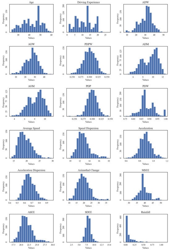
Figure 1.
Distributions of continuous variables.
4.3. Data Filling
By verifying each record in the dataset, 27 records with missing values of more than 50% of the feature variables were deleted, resulting in the retention of 1102 valid records. For the feature variables with fewer missing entries, this study utilized the plural, median, and mean to interpolate the missing values. For feature variables with a large amount of missing data (including the average speed, speed dispersion, etc.), these belonged to the non-random missing data of bus driver and driving vehicle matching. A single interpolation method was easy to weaken the internal feature information of the data.
Chained multiple interpolation usually performs well in dealing with complex, non-random, missing data, allowing for multiple variables to predict the missing values of a single variable. It also captures the relationship between the features, which is highly applicable to filling in non-random missing data [40,41]. The MICEForest multiple interpolation method is based on the chained multiple interpolation method and employs an ensemble of decision trees (random forests) to improve missing data processing for machine learning applications [42]. The random nature of the results obtained from the random forests makes it more sensitive to missing values, more resistant to interference, and a more accurate interpolation method [43]. Meanwhile, compared with other multiple interpolations, MICEForest can insert missing classification and regression data without too many settings, leading to faster fill rates [44]. Therefore, in this paper, the MICEForest multiple interpolation method was used to fill the missing values of the dataset. The interpolation process is the following:
- For datasets containing missing values, Ori_Datase, randomly select some values within the missing attribute columns to fill the missing values in those columns. This process generates a randomly completed dataset called “Rnd_dataset” and forms the correlation coefficient matrix “X_r.”
- Randomly choose a missing column from “Rnd_dataset”, referred to as an incomplete attribute column A. Use the non-missing values of A to form the training set and the missing values of A as the test set. Construct a random forest model to predict the missing values of A.
- Randomly select another attribute from the incomplete attributes, excluding A. Following the logic of the above filling missing value, iteratively impute the other incomplete attributes. This process creates the first iteration dataset “Dataset_0” and calculates the correlation coefficient matrix “X_0”.
- Use the convergence of correlation to determine whether “X_r” and “X_0” have converged. If they have not converged, return to step 2 and repeat the process, resulting in “Dataset_1” and correlation coefficient matrix “X_1”. Once convergence is reached, the final dataset “Dataset_0” is obtained.
- Repeat until n datasets are reached.
In this paper, the MICEForest multiple imputation method generated five datasets, each statistically compared with the original dataset. Figure 2 shows the average rate of change for each dataset after attributing missing attributes. Finally, according to the principle of taking the best value, the results of the same column in the five datasets were integrated to constitute the new complete dataset. At the same time, in order to verify the effectiveness, a dataset using mean imputation was also created. Both datasets were separately used in the prediction model.
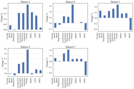
Figure 2.
Rates of change in mean values after interpolating missing attribute columns.
4.4. Correlation Analysis
In order to prevent the problem of covariance among independent variables, correlation analysis was performed for this paper. After removing some redundant features (correlation coefficients greater than 0.8), the feature set consisted of 24 features. The correlation analysis results for the remaining features are shown in Figure 3. Among them, the correlation between age and driving age (0.68) had the highest absolute value, but it was still less than 0.7, indicating that there was no longer a covariance problem between the independent variables.
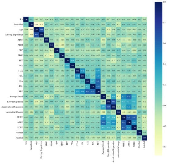
Figure 3.
Feature correlation heat map.
5. Methods
5.1. Boosted Trees
Boosted tree algorithms, represented by gradient-Boosted decision trees (GBDTs), are a very popular and effective class of algorithmic models used in machine learning today. They take gradient boosting as the core idea and build a powerful model by combining several weak learners (usually decision trees) [45]. Such algorithms inherit the good prediction effect and strong interpretability of decision trees, while improving the prediction speed and accuracy of the model [46,47]. The excellent learning properties of this class of machine learning algorithms were utilized. A suitable model was found based on accident data that had already occurred. Then, new data features were used to predict the objective function so as to achieve accurate prediction. Therefore, the traditional GBDT machine learning algorithm and three mainstream engineering implementation algorithms, eXtreme Gradient Boosting (XGBoost), light gradient-boosting machine (LightGBM), and categorical boosting (CatBoost), were selected to predict the risks of bus drivers.
5.1.1. GBDT
A GBDT is an iterative decision tree algorithm that constructs a strong learner by combining a set of weak learners (trees). The basic form of the model can be represented as
where is the final prediction; is the prediction of the m-th decision tree; and M is the total number of trees.
The core of a GBDT is the use of gradient descent to minimize a given loss function. For the m-th selection, the algorithm first computes the gradients of the loss function with respect to the current model prediction and then constructs a new decision tree to predict these gradients. The model update follows the following rules.
where is the learning rate, which controls the impact of each decision tree on the final prediction; is the predicted output of the model after m rounds of iterations; and is the predicted output of the weak learner obtained in the m-th round of iterations.
5.1.2. XGBoost
XGBoost is built on top of the standard gradient-boosting decision tree (GBDT) and introduces a regularization term to control the complexity of the model, thus preventing overfitting. Specifically, the objective function of XGBoost contains two parts: the training loss and the regularization term. Its form is as follows.
where represents the loss function for error between predicted and target values and represents the regularization term, used to control the complexity of the model, incorporating factors such as the number of trees, tree depth, etc.
5.1.3. LightGBM
Because XGBoost is always searching for the best split point of features during the decision tree splitting process, which leads to a large consumption of space and time during the operation process, LightGBM is proposed to address the shortcomings of XGBoost. LightGBM transforms the traversal of samples into the form of traversal histograms, which greatly reduces the time and space complexity in dealing with high-dimensional and massive data. It also integrates the exclusive feature bundling (EFB) algorithm with the one-sided gradient sampling algorithm (GOSS), which filters out the samples with a small gradient while realizing data dimensionality reduction and greatly saving time and space overheads. Its model can be expressed as the following:
where the weak learner in the current round to minimize the loss function.
5.1.4. CatBoost
CatBoost is a gradient-boosting decision tree (GBDT) framework whose main innovation lies in its efficient handling of categorization features. Unlike other algorithms in XGBoost and LightGBM, CatBoost utilizes symmetric decision trees (oblivious trees) to construct the base learner, which is an engineered implementation of GBDT with fewer parameters, support for category-type variables, and high accuracy. CatBoost also employs traditional gradient-boosting trees by minimizing the gradient descent loss function. The idea of training the model is such that when generating a new learner , is the negative gradient of the loss function in the current model.
From the above equation, it can be observed that there is a bias between the conditional distributions of and the training samples’ conditional distribution . Moreover, this bias becomes more pronounced as the dataset size decreases. CatBoost employs an ordered boosting technique (similar to the ordered TS method) to address this gradient bias and prediction shift issue, which may make CatBoost outperform other GBDT models on specific datasets.
5.1.5. Evaluation
The problem of predicting the risk of accidents for bus drivers with the target variable of whether or not an accident occurs in the current month is a typical binary classification problem. A confusion matrix is one of the most basic tools for assessing the effectiveness of classification in binary classification problems. It classifies the actual observations according to the predicted categories into the following: true-positive (TP), the number of samples predicted to be positive and actually positive; false-positive (FP), the number of samples predicted to be positive but actually negative; true-negative (TN), the number of samples predicted to be negative and actually negative; and false-negative (FN), the number of samples predicted to be in the minus category but actually in the plus category. This is shown in Table 2.
Table 2.
Confusion matrix.
The confusion matrix provides us with a comprehensive view of model performance. Based on the four metrics in the confusion matrix, multiple evaluation metrics can be computed to understand how the model performs in different aspects.
Precision—This is concerned with the proportion of positive cases that the model predicts will actually be positive. It provides a measure of how accurately the model predicts “positive cases” (in this case, accurately predicting accidents).
Recall—The main focus is on the proportion of positive examples that the model is able to identify out of the entire set of positive examples. It measures the ability of the model to identify all actual positive example samples (to predict all transit crashes).
F1-score—This is a metric that combines precision and recall and provides an assessment of the balance of the model.
ROC curve—This focuses on the ability of the model to distinguish between positive and negative cases. It is a performance curve plotted at different thresholds with a true-positive rate (TPR) on the vertical axis and a false-positive rate (FPR) on the horizontal axis.
AUC value—This is the area under the ROC curve; the closer the AUC value is to 1, the better the model performance.
PR curve—The horizontal axis indicates recall and the vertical axis indicates precision; by plotting the performance curve of the model under different thresholds, it brings more attention to the balance between the precision and recall of the model under different thresholds.
AUC-PR—This is the area under the PR curve; the closer the AUC-PR is to 1, the better the model can balance precision and recall under different thresholds.
Cohen’s kappa (k)—This is a metric that provides an assessment of the degree of agreement between the classifier’s predictions and actual observations. A Cohen’s kappa (k) < 0.00 indicates that the model classifies poorly, 0.00–0.20, slightly, 0.21–0.40, fairly, 0.41–0.60, moderately, 0.61–0.80, substantially, and 0.81–1.00, almost perfectly.
5.2. Bayesian Hyperparametric Optimization
Different tasks and datasets exhibit varied sensitivities toward hyperparameters, influencing model learning efficiency, complexity, capacity balance, etc. [48]. For instance, the learning rate plays a pivotal role in determining the step size in gradient descent algorithms, which is crucial for minimizing the loss function. Properly balancing a learning rate is essential to ensuring the convergence of gradient descent toward the minimum without facing overly slow convergence or overshooting the minimum [49,50]. A reasonable selection of hyperparameters significantly augments a model’s predictive and generalization capabilities, ultimately enhancing its practical applicability [51]. This study delves into pivotal parameters impacting the CatBoost model and a Bayesian hyperparameter optimization approach was employed to fine-tune the model’s performance.
Bayesian optimization is a black-box-based method for globally optimizing an objective function, which constructs a posterior distribution for the objective function and uses Gaussian process regression to compute the uncertainty in the distribution, and then uses an acquisition function to decide where to sample. The iterative approach is to complete the first evaluation and then find the next evaluation point for the second evaluation, and so on. Given the objective function to be optimized was (AUC-PR in this paper), then, according to this objective function, the optimization problem to be solved can be expressed as the following:
where denotes the given hyperparameter search space; denotes the combination of hyperparameters obtained by searching in the given hyperparameter search space with the objective of minimizing ; and denotes the objective function.
The Bayesian formulas used are the following:
where denotes the objective function to be optimized; denotes the sample points selected from the parameter space with their corresponding objective function values into the dataset, where i = 1, 2, ...n; denotes the likelihood distribution of y; denotes the prior probability distribution; is the marginal likelihood distribution of the marginalized ; and is the posterior probability distribution of the objective function, and the use of posterior probability distributions could be computed to the acquisition function to determine the next set of assessment points to be used for evaluation.
5.3. Interpretable SHAP Methods
The interpretable SHAP method is a TreeExplainer method based on the SHAP value in game theory [52]. The core idea is to compute the marginal contribution of the features to the model’s output and then interpret the “black-box model” on this basis, both at the overall level and at the local level [53]. This value provides information about how predictions are fairly distributed among features.
The main definition of the Shapley value is
For the subset of risk factors (where represents the set of all risk factors and S is the subset of features), two models were trained to extract the impact of factor i. The first model was trained on the set of coalitions without factor i. The first model inputted the probability of accidents under factors i and S, while the other trained the set of coalitions without factor i. The first model inputted the probability of accidents under factor i and represents the weight of this coalition. is the Shapley value for factor i.
In SHAP, all input features of a machine learning model are considered as “contributors” to the final prediction and are evaluated based on their individual impact on the output [53]. Assuming that the i-th sample is and the j-th feature of the i-th sample is , Shapley obeys the following equation:
where represents the j-th feature of the i-th sample; represents i-th sample’s predicted value; denotes the SHAP value of , which represents the contribution of the j-th feature to the final predicted value and if , it indicates that the feature has a positive impact on the prediction, and vice versa if it is negative.
6. Results
6.1. Model Comparison
Features in the new complete dataset were used as inputs for the model. Whether a bus driver had been involved in an accident was taken as the model’s output. The data were split into a training set and a test set in a ratio of 7:3. The training set was utilized in each of the four algorithms mentioned in Section 5.1, with a 10-fold cross-validation method. The test set of data was evaluated using the evaluation indicators listed in Section 5.1.5. The evaluation results are shown in Table 3 and Table 4. At the same time, the ROC curves and PR curves of the four models on the test set are plotted, as shown in Figure 4 and Figure 5.
Table 3.
Confusion matrix for four models.
Table 4.
Results of the model evaluation of the four methods.
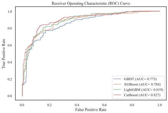
Figure 4.
Comparison of ROC curves for four models.
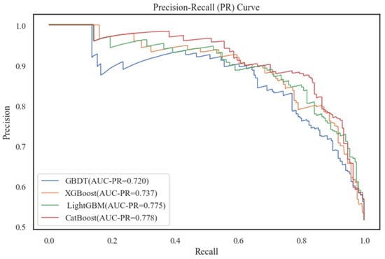
Figure 5.
Comparison of PR curves for four models.
From combining the scores of each evaluation metric on each model, CatBoost performed outstandingly on both the training set and the test set, whose scores were significantly higher than others. The LightGBM model also performed well, but not as much as CatBoost. This was followed by XGBoost, and the GBDT model performed the worst. CatBoost performance on precision and recall showed that it was able to be more accurate in predicting the occurrence of bus driver accidents. The F1-score also demonstrated the model’s better balanced results in terms of both accuracy and coverage. Cohen’s kappa (k) was greater than 0.6, which indicates the model’s substantial consistency in terms of prediction results and actual observations. In addition, Figure 4 and Figure 5 show that the ROC curve and PR curve of CatBoost are significantly higher than the other three models, and the AUC and AUC-PR are also the largest. They also show that the algorithm had a very good classification performance for the target variables on the test subset, and it could more accurately differentiate the accident occurrence of bus drivers. Therefore, the CatBoost algorithm was selected for bus drivers’ probability prediction in this paper.
6.2. Bayesian Hyperparameter Optimization
In this study, the Bayes_opt library of Python was used for hyperparameter optimization, in aiming to find a better fitted model. The existing research focuses more on cases of bus drivers having accidents. Therefore, the performances of different hyperparameter combinations on the validation set were evaluated using the average area under the exact recall curve (AUC-PR) as the optimization objective, along with 10-fold cross-validation. The search range of the optimization parameters used in this paper and the optimal hyperparameter combinations are shown in Table 5. The number of iterations is 600, and the optimization process is shown in Figure 6. The straight line in the figure is the fitted straight line between iterations and the AUC-PR, from which it can be seen that the AUC-PR value shows an obvious upward trend with the growth of iterations. This trend indicates that the Bayesian hyperparameter optimization method was trying the optimal hyperparameter combinations continuously. Moreover, the AUC-PR value reached the optimal value of the whole search process at the 284th iteration. Eventually, the optimal AUC-PR value reached 0.828, which was 6.73% higher compared with the default parameter.
Table 5.
Parameters and optimization ranges and results.
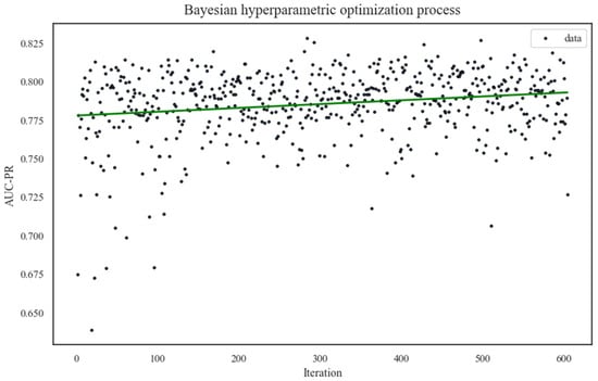
Figure 6.
Bayesian optimization process.
6.3. CatBoost Prediction Results
Based on the optimal parameters by the Bayesian hyperparameters, the model was retrained on the training set. The final effect was evaluated on the test set, which can be seen in Table 6. The optimized CatBoost model more accurately distinguished the accident probability of bus drivers. It is obvious that all the model metrics improved, and especially, the false-positive and false-negative cases in the confusion matrix are significantly reduced. Cohen’s kappa (k) increased most outstandingly to 0.680 (0.61–0.80, substantially). Compared to the default parameter CatBoost, it improved by 0.025 with an increase of 3.82%, by 6.75% compared to LightGBM, by 18.06% compared to XGBoost, and by 24.54% compared to GBDT. The values of AUC and AUC-PR also obviously increased with 0.834 and 0.788, respectively. Particularly, the values for the AUC-PR improved, by 1.29% compared to the default parameter, by 1.68% compared to LightGBM, by 6.92% compared to XGBoost, and by 9.44% compared to GBDT. These all indicate that the optimized model minimized false alarms while accurately identifying the occurrence of accidents, making the model more accurate and robust.
Table 6.
Final evaluation results.
Figure 7 and Figure 8 demonstrate the statuses of the ROC and ROC-PR curves of the CatBoost model before and after Bayesian tuning of the different interpolated datasets. The conclusions that can be drawn are the following:
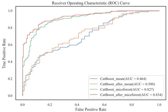
Figure 7.
Comparison of ROC curves for different interpolated datasets.
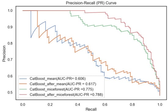
Figure 8.
Comparison of PR curves for different interpolated datasets.
- I)
- The estimated datasets obtained using the mean imputation method or the MICEForest multiple imputation method have higher ROC and ROC-PR curves after Bayesian hyperparameter tuning. This points to the Bayesian optimization-based tuning process effectively having improved the model’s robustness and predictive ability. This finding verifies the scientific validity and reasonableness of the Bayesian hyperparameter optimization method and provides an intuitive validation of the model’s performance improvement.
- II)
- The ROC and ROC-PR curves of the MICEForest multiple imputation method are remarkably higher than those of the mean imputation method, regardless of whether Bayesian hyperparameters adjusted the MICEForest multiple imputation method. This observation implies that MICEForest multiple imputation minimizes the loss of data information to a greater extent, resulting in more reliable imputed data. Meanwhile, this result implies that for model performance improvement, data integrity and quality are important, and the MICEForest multiple interpolation method has a better effect and reliability in data interpolation.
In summary, the Bayesian hyperparameter optimization process enhanced the model’s performance. MICEForest multiple imputations provided more reliable and informative data for building the predictive model, supporting the validity and superiority of the CatBoost model used for the prediction of the probability of accidents occurring among bus drivers.
6.4. SHAP Analysis
Prior research has identified correlations between accident occurrence and various factors, including but not limited to individual bus driver characteristics, work hour characteristics, violation and risky behavior characteristics, and so on. Despite this prior knowledge, the exact influence of these characteristics on the probability of accidents still needs to be determined. At the same time, the CatBoost model constructed in the previous section is a black-box model, which does not clearly show the mechanism of the influence of each characteristic on the probability of accidents. Therefore, the SHAP interpretable method was adopted in this paper to visualize and interpret the CatBoost results.
Figure 9 displays the average contributions of every feature. The horizontal axis is each feature’s average absolute SHAP values, representing their impact on the prediction variable. The vertical axis is arranged according to the importance of the variables, with higher positions indicating more significant influence. In Figure 9, the features “Age” and “Rainfall” are ranked at the top, with average SHAP values of 0.11 and 0.1, respectively, significantly surpassing the other features. This suggests that age and rainfall are strongly related to the accident risk of bus drivers. The next are “Driving Experience” and “Azimuthal Change”. Following that are driving characteristics (e.g., “the proportion of driving duration during peak duration” (PDP), “the accumulated driving duration of the previous week” (ADW), and “the proportion of driving duration within the week” (PDW)), operational characteristics (e.g., “speed dispersion when entering and exiting stations” (SDEE) and “Average Speed”), as well as the “time since last violation” (TLV) and “Education”.

Figure 9.
Feature importance ranking chart.
Figure 10 shows the relationships between the features and the predicted target variables. It covers the SHAP values of each feature for each sample. The colors represent the magnitude of the feature value (red indicates a higher feature value and blue indicates a lower feature value) and the horizontal axis indicates the importance of the influence on the target variable, shown as a SHAP value. For example, the red dots for age and driving age are mainly located on the left side of the horizontal axis, which indicates that when the eigenvalues of the age and driving age variables of the bus drivers were large, the impact on the model was relatively tiny (the SHAP values are negative). This means that the older the bus driver’s age and driving age are, the less likely that accidents will occur. This impact on the model was relatively small, which means that the older the bus driver is, the lower the probability of an accident. Similarly, the red dots, according to the length of the last violation, azimuth change, etc., are mainly located on the right side of the horizontal axis, indicating that the longer the bus driver has gone since the last violation and the greater the degree of change in their azimuth angle, the greater the possibility that the bus driver will be involved in an accident.
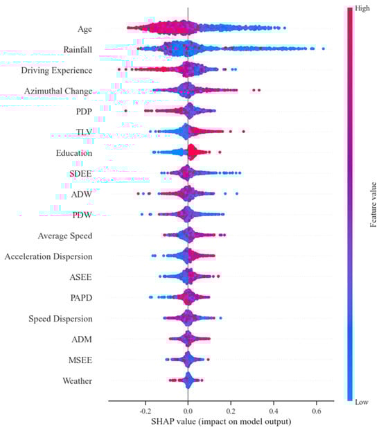
Figure 10.
SHAP summary plot.
To further explore the relationship between bus driver accident risk and each feature, SHAP dependency plots were plotted for the top 12 ranked features, as shown in Figure 11. Each point in the plot is a sample. The histogram shows the distribution of each feature, while the trends visualize the impact of the variables on the model output. By analyzing the trends and patterns of the sample points in the plots, we can better understand how each feature contributes to the overall risk.
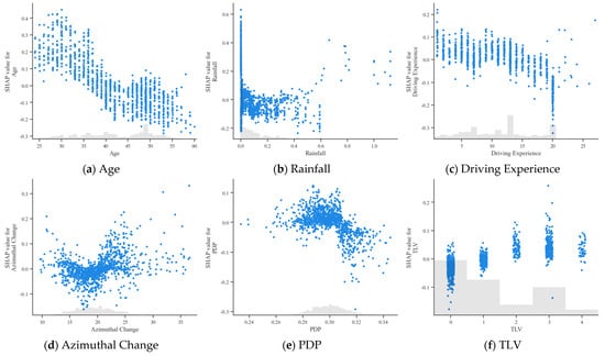
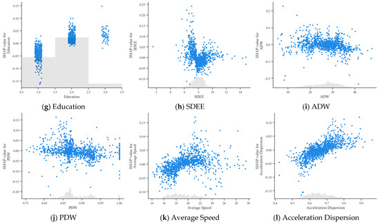
Figure 11.
SHAP dependency graphs.
Regarding the features “Age” and “Driving Experience”, as the age and driving experience of bus drivers increase, their SHAP values gradually decrease from positive to negative. This revealed that younger and less experienced bus drivers tend to have a higher accident risk. For bus drivers above 45 years with driving experience exceeding 15 years, their SHAP values remain negative and stable, indicating a relatively low accident risk in this category. Regarding the “Education” feature, most bus drivers have an educational level of 1 or 2, corresponding to primary or high school education. The risk level was the lowest when the educational level was at 1.
For the “Rainfall” feature, many samples are clustered around 0. This is related to the weather in June in Chongqing Municipality, where there was no rainfall or less rainfall for most of the time. When the rainfall was less than 0.3 mm/h, its SHAP value was mostly less than 0, and the driver’s risk level was relatively low and safer. When the “Rainfall” was less than 0.5 mm/h (i.e., light rain or less), the driver’s risk level was low. Then, as rainfall exceeded, the SHAP value increased, meaning a positive relationship between rainfall and the accident risk of bus drivers.
For the “Azimuthal Change” feature, when the azimuthal change was less than 20, most of the SHAP values were negative, clearly showing that more minor azimuthal changes were associated with lower accident risk for bus drivers. After that, the more significant the change in azimuth, the higher the accident risk.
For PDP, the plot shows that when the proportion of driving time during peak hours was less than 0.3, the SHAP values fluctuated around 0, but were mostly greater than 0, showing a positive effect on the impact of accidents. Yet, when the proportion exceeded 0.3, the SHAP values decreased.
For TLV, as the value of the horizontal coordinate increased, the longer the bus driver was from the last violation. As can be seen from the figure, there was a dampening effect on bus driver risk the shorter the length of time since the previous offense (within one week). As the length of time increased, the risk of bus drivers gradually increased. However, the probability of accidents for bus drivers who had not had a violation within six months was also low.
For SDEE, when the value of the entry and exit speed discrepancy was around 8, its SHAP value was less than 0, indicating that it has a particular inhibitory effect on accident risk. As the discrepancy increases and decreases, the accident risk shows an upward trend.
For ADW and PDW, the cumulative driving time of bus drivers in the last week was mostly around 30 h, and their driving time per day did not vary much, with their SHAP values more centrally distributed around zero. For PDW, most of the surveyed bus drivers had some non-working days in their driving experience. The SHAP values also fluctuated around 0 and remained relatively stable.
In addition, four feature combinations with significant interactions were selected to explore the interaction between bus driver accident features, as shown in Figure 12. Compared with the SHAP dependency graphs, the feature interaction graphs have a colored bar on the right side, which indicates the value of another feature interacting with the current feature.

Figure 12.
Partial characteristic influence interaction diagrams.
In Figure 12a, it can be seen that the higher the “Age” of the bus driver, the higher his or her “Driving Experience”. In the red section on the right, higher aged drivers have negative SHAP values with high driving experience, showing a negative influence effect. Meanwhile, the blue scatter on the left shows that low driving experience has a positive SHAP for low age, showing a positive influence effect.
In Figure 12b, at one month or more from the last violation (taking the values of 2, 3, and 4), the increment of PDP increased the SHAP value of the TLV, showing its positive influencing effect. Instead, when the length of time since the last violation was more than six months, the increment of PDP decreased the SHAP value of the TLV.
Similarly, in Figure 12c, the increase in age increased the SHAP value of education when the education level was 2, while it had a negative effect when the education level was elementary school.
Figure 12d shows an interaction effect between the PDW and age. When the proportion of driving time during weekdays was less than 0.87, there was no significant change in the accident risk of bus drivers. However, when the proportion exceeded 0.87, different age groups of drivers showed a significant difference in accident risk. With a higher number of driving hours during the week, the accident risk for older bus drivers decreased, while the accident risk for younger bus drivers remained high. As the PDW got higher (closer to 1), the SHAP of the red point was less than 0. Older drivers reduced the SHAP value of the PDW. In other words, increasing age minimized the effect of PDW on accidents.
In addition to the previous analysis, this study further compared the risk profiles of bus drivers by plotting the feature impact heat maps for samples with the label 1 (Figure 13a) and label 0 (Figure 13b). The x-axis represents the sample sequence with data points below. The color of each data point stands for the magnitude of its feature value, signifying the degree of influence on the accident risk. The red represents a higher feature value, showing a positive impact relationship. Taking “Rainfall” as an example, approximately 0–180 samples in Figure 13a and 0–20 samples in Figure 13b are shown in red, indicating that these bus drivers were strongly affected by higher rainfall. At the same time, it can be visualized that Figure 13a is dominated by red and Figure 13b is primarily blue, demonstrating that features for drivers in group (a) have a positive correlation with their risk level, while features for drivers in group (b) have a negative correlation.
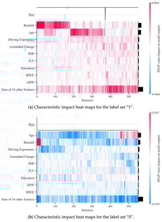
Figure 13.
Maps of different tag set features.
Furthermore, the y-axis is sorted based on the importance of the features. It is noted that there are slight differences in the impact features between the different categories of drivers. In Figure 13a, the variables “Rainfall” and “SDEE” have a more prominent impact compared to Figure 13b. This difference points out that compared to bus drivers with a lower accident risk, “Rainfall” and “SDEE” play a more significant role in predicting the accident risk for bus drivers with a higher risk.
The variation in the impacts of different features between the two driver categories provides valuable insights into the factors contributing to higher accident risk in certain drivers. By understanding these differences, appropriate measures and interventions can be developed to improve road safety and reduce the occurrence of bus accidents.
The SHAP interpretability method not only visualizes the accident propensity of a population of bus drivers, but for a single sample (i.e., a single bus driver), it also shows the mechanism by which their characteristics influence the occurrence of accidents. Figure 14 is a waterfall diagram used to locally interpret a positive and negative sample (selected using simple random sampling). Each arrow indicates the direction and magnitude of the feature’s effect on the target. The graph starts at the bottom with the expected value predicted by the model and progressively shows the contribution of each feature to the expected value. Based on the principle of linear additivity, the results of each feature’s contribution were added together to provide the final prediction.
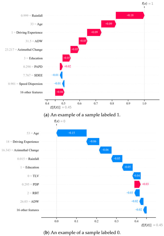
Figure 14.
Waterfall diagrams with different labels.
As shown in Figure 14, the primary factors and their levels of importance are distinct for different drivers. In Figure 14a, the indicators that had a more significant impact on accident probability for the bus driver were rainfall, 0.99, age, 33, driving experience, 1, ADW, 31.5, etc., and most features had a positive effect. With these features’ positive and negative effects, the model predicted a result of 1 for this driver, implying that an accident would occur. In contrast, in (b), the most influential indicator was an age of 53, whereas factors such as a rainfall of 0.051, driving experience of 18, and ADW of 26.03, etc., turned into adverse effects. Therefore, utilizing this local interpretation method of SHAP is necessary, which provides accident propensity analysis results for each driver. Such targeted analysis results can help bus drivers precisely understand their risk propensity and vulnerability characteristics. This approach allows them to identify and improve their potential safety blind spots for more targeted self-assessment and training. At the same time, it also provides decision support for relevant companies to formulate more effective safety strategies and management programs.
7. Discussion
This study focused on a predictive model for bus driver accident risk and analyzed the main influencing factors and mechanisms through interpretability results.
By comparing it with three mainstream ensemble learning models, GBDT, XGBoost, and LightGBM, CatBoost was utilized to build a predictive model, and its effectiveness in predicting bus driver accident risk was verified. The well predictive performance of CatBoost was consistent with previous research [54,55,56].
With Bayesian hyperparameter optimization, the predictive power and robustness of the CatBoost model were effectively enhanced. It achieved an AUC of 0.834, an AUC-PR of 0.788, and a Cohen’s kappa (k) of 0.68 on the test set, improvements of 0.85%, 1.29%, and 3.82%, respectively, over the default parameters. The reliability of Bayesian hyperparameter optimization has also been confirmed in previous studies [49,57,58].
The visualization of the model made by SHAP revealed 12 critical indicators with a high impact on the risk. By comparing the findings with previous research, both similarities and differences were identified, allowing for further insights to be gained.
In terms of individual characteristics, age and driving experience showed a similar influence trend. As age and driving experience increase, accident risk decreases, which aligns with previous findings [59]. This could be attributed to the fact that older drivers tend to have a more composed mindset and a milder driving style, exhibiting higher levels of safety. Likewise, drivers with higher driving experience are at lower risk probably because of their better driving skills and wealth of experience [60]. But in contrast, the findings regarding bus drivers’ education level in this study differ from a previous conclusion [61]. Drivers with a higher level of education (categorized as 3) showed a higher level of risk. One reason for this may be the considerable variation in the number of bus drivers with different levels of education, especially since the more educated drivers (categorized as level 3) made up only 5% of the dataset. Another reason may be that this segment of bus drivers tends to be younger and more susceptible to the higher importance factor “Age”, as shown in Figure 12c. However, this result also emphasizes the skill-based nature of the bus driver occupation, which means that a bus driver’s driving operational skills and proficiency under different road conditions, as opposed to theoretical knowledge, more profoundly affect the safety of their bus operations.
Undoubtedly, the current day’s rainfall is the most important factor. This has been proven by Nguyen T C [62] and Zhou H [63]. Our study found that bus drivers’ accident risk tended to increase during moderate rain or more. This phenomenon could be attributed to the condition of the road surface. When it is drizzly, there is only a slight change in road surface humidity, while as the rainfall continues to increase, completely wet pavements or even puddles lead to a sharp decrease in the friction coefficient. Vehicles are more prone to sideslip in this environment, triggering traffic accidents. Simultaneously, heavy rainfall affects drivers’ visibility and judgment, reducing their perception of surrounding conditions and unexpected situations, which can compromise driving safety. Additionally, bus drivers’ accident risks diverge when rainfall is close to zero. Some drivers show relative safety, while the risk of accidents for other public transport drivers increases instead. This disparity implies a lesser impact of rainfall under favorable driving conditions, showing the heterogeneity among individuals.
The correlation between the driving duration of bus drivers and their accident risk has been confirmed, consistent with previous studies [5,39]. Among our studies, the most notable is the proportion of peak driving duration (PDP). The accident risk of bus drivers was higher when their peak driving hours were under three hours (peak driving hours as a percentage of less than 0.3). The nature of the peak hour determined this phenomenon, in which the increased interferences and driving pressures led to a higher likelihood of collisions. Another aspect is that when the daily peak driving duration exceeded three hours, the accident risk of bus drivers decreased. This could be attributed to bus drivers often working across multiple peak periods within one day, resulting in a shorter average peak driving duration in each period, leading to more focused attention. This conclusion can help companies rationalize the work schedule of bus drivers and reduce the impact of peak periods of their driving. Additionally, the accident risk of bus drivers is also influenced by their driving duration on non-working days, reflected in the proportion of driving duration within the week (PDW). At high percentages of weekday driving, a significant difference for bus drivers of different ages was observed, with older drivers having a lower risk of accidents. For good reasons, older drivers are more comfortable with regularity and are better able to perform driving tasks than younger drivers. To address these findings, management authorities could refine their control strategies, optimizing internal periodic scheduling, which would help maximize the advantages of each category and achieve targeted administration. Moreover, the accumulated driving duration of the previous week (ADW) is also related to the occurrence of accidents, especially in terms of its effect on a single transit driver. The opposite impact relationship of (ADW) on accidents for two bus drivers in Figure 14a,b is very noteworthy. This requires management to rationalize bus drivers’ working hours to control this feature’s effect on accidents.
Previous studies have indicated a significant correlation between the historical violation characteristics of bus drivers and their accident risks [61,64]. Within this study, the feature significantly associated with the risk of bus drivers was the duration since the last violation. As this duration increased, the risk for bus drivers gradually increased. The potential cause might be attributed to the impact of criticism or education of drivers who have recently been involved in accidents or penalized for violations. Such interventions tend to heighten their attention, leading to a more conservative driving style and greater adherence to traffic rules, consequently reducing the probability of accidents. Conversely, with a longer duration since the last violation, a driver’s alertness diminishes, behavioral constraints loosen, and accidents often occur due to negligence. Moreover, bus drivers without violations within six months had a notably low probability of accidents. This highlights that bus drivers who consistently maintain a good driving record over an extended period exhibit a relatively stable accident risk, further affirming the close link between violations and accidents.
Bus drivers’ entry and exit operations are essential components of their daily work, and their status is tightly aligned with the security of their own and passengers’ journeys. Zhou [63] established that passengers are likelier to lose balance during boarding and alighting, making them susceptible to fatal injuries in non-collision incidents. In this study, the differences in the importance of features also shown in Figure 13a,b indicate their weightiness. The characteristic accident risk was suppressed when the degree of in/out station speed dispersion was in the normal range (taking the value of 8). Below or above the normal range, the accident risk increased. This safety threshold range reveals the stability regularity of a driver’s driving, which can assist the government in monitoring their driving status and preventing potential safety accidents.
The key indicators that influence their accident risk are azimuthal change, acceleration dispersion, and average speed. This relationship has also been consistently found in the research [65,66]. This study confirmed the positive correlation between these three indicators and bus driver accidents. For bus drivers, frequent azimuthal changes may have increased a driver’s operating difficulty and attention burden, especially when frequent lane changes or crossing complex intersections were required. Frequent speed changes can disrupt the order of traffic flow on the road, which is more likely to lead to tailgating and scraping accidents. The phenomenon that higher average speeds increase the possibility of accidents is evident in the complex environment of urban roads.
In this paper, a reliable analysis and prediction method for bus drivers based on their occupational driving characteristics was designed. The data were all from the daily regulatory data of bus companies. The features were derived from information collected by the companies in driver profile development and daily transportation. Using daily data to predict accident probabilities provides a practical method for bus companies, allowing for the efficient reuse of data resources. In addition, the SHAP interpretive method can help mine the characteristic tendencies and visualize the influence mechanism of group bus drivers. In practical application, it can also analyze the risk propensity of individuals at a certain point in time (excluding the transportation process). For example, track and working data can be retrieved before the end of the day and then integrated with future scheduling conditions and climatic conditions of individual drivers to their accident propensity. This method can provide differentiated supervision for drivers in their next driving exercise and improve supervision targeting. In this way, it can improve the safety management level of public transportation operations and ensure urban road safety.
8. Conclusions
This research developed a model for predicting and analyzing the probability of accidents among bus drivers, taking into account their occupational characteristics. The main conclusions are the following:
- The CatBoost method was used for bus driver accident probability prediction. The missing data were filled in based on the MICEForest multiple interpolation method. The CatBoost model was adjusted by the Bayesian hyperparameter optimization method with AUC-PR as the optimization objective. After optimization, the prediction model reached an AUC of 0.834, an AUC-PR of 0.788, and a Cohen’s kappa (k) of 0.68 for the test set. They were 1.83%, 1.68%, and 6.79% higher than LightGBM, respectively, 5.84%, 6.92%, and 18.06% higher than XGBoost, respectively, and 7.89%, 9.00%, and 9.00% higher than GBDT, respectively. Meanwhile, the MICEForest interpolated dataset had a significant advantage over the single mean computation method, as evidenced by the ROC and PR curves.
- The predictive model was explained by the SHAP interpretable method. The most important features were age and daily rainfall. Next, came driving experience, azimuthal change, etc. In addition, this study innovatively found that the peak driving duration, the degree of dispersion of entry and exit speeds, the duration of the last violation, and the weekday driving duration of a bus driver are related to their accident risk. These results were also discussed and visualized with the help of SHAP, regarding group and individual accident probability mechanisms, interaction effects between the features, and accidental and non-accidental group accident tendencies.
In conclusion, this study provides a more scientific method and valuable insights for predicting the probability of bus driver accidents. It is significant for related companies to identify the potential risks of bus drivers, scientifically adjust drivers’ work schedules, and promptly formulate cyclical education and training strategies. However, there are some limitations; for example, only one month of bus driver accident data in one region were selected, resulting in a single environment. This is because the state-funded project this paper relied on is still in progress, and more data are yet to be available. But, as the project demonstration progresses, we will collect more cities and a more extended sample dataset. This expansion will help in assessing the model’s predictive power and adaptability more accurately. At the same time, we will consider adding more features that affect the probability of bus driver accidents to provide more theoretical support and practical guidance for accident risk prevention and control.
Author Contributions
Conceptualization, T.D., L.Y., J.X. and K.Z.; methodology, T.D. and L.Y.; formal analysis, T.D. and K.Z.; writing—original draft, L.Y. and K.Z.; writing—review and editing, T.D., L.Y. and J.X.; supervision, J.X.; data curation, Z.L.; project administration, T.D., Z.L. and J.X. All authors have read and agreed to the published version of the manuscript.
Funding
This research was funded by the National Key R&D Program of China (2021YFC3001500) and Scientific and the Jilin Province Transportation Innovation Development Support Project titled ‘Dynamic Evaluation Technology Research for Rural Road Development in Jilin Province’.
Institutional Review Board Statement
Not applicable.
Informed Consent Statement
Not applicable.
Data Availability Statement
The data presented in this study are available on request from the corresponding author. The data are not publicly available due to privacy.
Conflicts of Interest
The authors declare no conflicts of interest.
References
- Alkaabi, K. Identification of hotspot areas for traffic accidents and analyzing drivers’ behaviors and road accidents. Transp. Res. Interdiscip. Perspect. 2023, 22, 100929. [Google Scholar] [CrossRef]
- Liou, J.J.H.; Liu, P.C.Y.; Luo, S.-S.; Lo, H.-W.; Wu, Y.-Z. A hybrid model integrating FMEA and HFACS to assess the risk of inter-city bus accidents. Complex Intell. Syst. 2022, 8, 2451–2470. [Google Scholar] [CrossRef]
- Bhandari, R.; Raman, B.; Padmanabhan, V.N. FullStop: A Camera-Assisted System for Characterizing Unsafe Bus Stopping. IEEE Trans. Mob. Comput. 2020, 19, 2116–2128. [Google Scholar] [CrossRef]
- Wang, Q.; Zhang, W.; Yang, R.; Huang, Y.; Zhang, L.; Ning, P.; Cheng, X.; Schwebel, D.C.; Hu, G.; Yao, H. Common Traffic Violations of Bus Drivers in Urban China: An Observational Study. PLoS ONE 2015, 10, e0137954. [Google Scholar] [CrossRef] [PubMed]
- Hanumegowda, P.K.; Gnanasekaran, S. Prediction of Work-Related Risk Factors among Bus Drivers Using Machine Learning. Int. J. Environ. Res. Public Health 2022, 19, 15179. [Google Scholar] [CrossRef] [PubMed]
- Maghsoudipour, M.; Moradi, R.; Moghimi, S.; Ancoli-Israel, S.; DeYoung, P.N.; Malhotra, A. Time of day, time of sleep, and time on task effects on sleepiness and cognitive performance of bus drivers. Sleep Breath. 2022, 26, 1759–1769. [Google Scholar] [CrossRef]
- Jakobsen, M.D.; Glies Vincents Seeberg, K.; Møller, M.; Kines, P.; Jørgensen, P.; Malchow-Møller, L.; Andersen, A.B.; Andersen, L.L. Influence of occupational risk factors for road traffic crashes among professional drivers: Systematic review. Transp. Rev. 2023, 43, 533–563. [Google Scholar] [CrossRef]
- Alver, Y.; Demirel, M.C.; Mutlu, M.M. Interaction between socio-demographic characteristics: Traffic rule violations and traffic crash history for young drivers. Accid. Anal. Prev. 2014, 72, 95–104. [Google Scholar] [CrossRef]
- Tavakoli Kashani, A.; Besharati, M.M. An investigation of the relationship between demographic variables, driving behaviour and crash involvement risk of bus drivers: A case study from Iran. Int. J. Occup. Saf. Ergon. 2021, 27, 535–543. [Google Scholar] [CrossRef]
- Goh, K.; Currie, G.; Sarvi, M.; Logan, D. Factors affecting the probability of bus drivers being at-fault in bus-involved accidents. Accid. Anal. Prev. 2014, 66, 20–26. [Google Scholar] [CrossRef]
- Anund, A.; Ihlström, J.; Fors, C.; Kecklund, G.; Filtness, A. Factors associated with self-reported driver sleepiness and incidents in city bus drivers. Ind. Health 2016, 54, 337–346. [Google Scholar] [CrossRef] [PubMed]
- Useche, S.A.; Ortiz, V.G.; Cendales, B.E. Stress-related psychosocial factors at work, fatigue, and risky driving behavior in bus rapid transport (BRT) drivers. Accid. Anal. Prev. 2017, 104, 106–114. [Google Scholar] [CrossRef] [PubMed]
- Elvik, R. Driver mileage and accident involvement: A synthesis of evidence. Accid. Anal. Prev. 2023, 179, 106899. [Google Scholar] [CrossRef]
- Blower, D.; Green, P.E. Type of Motor Carrier and Driver History in Fatal Bus Crashes. Transp. Res. Rec. 2010, 2194, 37–43. [Google Scholar] [CrossRef]
- Feng, S.; Li, Z.; Ci, Y.; Zhang, G. Risk factors affecting fatal bus accident severity: Their impact on different types of bus drivers. Accid. Anal. Prev. 2016, 86, 29–39. [Google Scholar] [CrossRef]
- Huting, J.; Reid, J.; Nwoke, U.; Bacarella, E.; Ky, K.E. Identifying Factors That Increase Bus Accident Risk by Using Random Forests and Trip-Level Data. Transp. Res. Rec. 2016, 2539, 149–158. [Google Scholar] [CrossRef]
- Samerei, S.A.; Aghabayk, K.; Mohammadi, A.; Shiwakoti, N. Data mining approach to model bus crash severity in Australia. J. Saf. Res. 2021, 76, 73–82. [Google Scholar] [CrossRef]
- Zhu, T.; Qin, D.; Wei, W.; Ren, J.; Feng, Y. Research on accident risk identification and influencing factors of bus drivers based on machine learning. Chin. J. Saf. Sci. 2023, 33, 23–30. (In Chinese) [Google Scholar]
- Gehlert, T.; Hagemeister, C.; Özkan, T. Traffic safety climate attitudes of road users in Germany. Transp. Res. Part F Traffic Psychol. Behav. 2014, 26, 326–336. [Google Scholar] [CrossRef]
- Chu, W.; Wu, C.; Atombo, C.; Zhang, H.; Özkan, T. Traffic climate, driver behaviour, and accidents involvement in China. Accid. Anal. Prev. 2019, 122, 119–126. [Google Scholar] [CrossRef]
- Deng, S.; Yu, H.; Lu, C. Research on operation characteristics and safety risk forecast of bus driven by multisource forewarning data. J. Adv. Transp. 2020, 2020, 6623739. [Google Scholar] [CrossRef]
- Fu, X.; Xu, C.; Liu, Y.; Chen, C.-H.; Hwang, F.; Wang, J. Spatial heterogeneity and migration characteristics of traffic congestion—A quantitative identification method based on taxi trajectory data. Phys. A Stat. Mech. Its Appl. 2022, 588, 126482. [Google Scholar] [CrossRef]
- Bhandari, R.; Raman, B.; Padmanabhan, V.N. FullStop: Tracking unsafe stopping behaviour of buses. In Proceedings of the 2018 10th International Conference on Communication Systems & Networks (COMSNETS), Bengaluru, India, 3–7 January 2018; pp. 65–72. [Google Scholar]
- Jeong, H.; Kim, I.; Han, K.; Kim, J. Comprehensive Analysis of Traffic Accidents in Seoul: Major Factors and Types Affecting Injury Severity. Appl. Sci. 2022, 12, 1790. [Google Scholar] [CrossRef]
- AlMamlook, R.E.; Kwayu, K.M.; Alkasisbeh, M.R.; Frefer, A.A. Comparison of Machine Learning Algorithms for Predicting Traffic Accident Severity. In Proceedings of the 2019 IEEE Jordan International Joint Conference on Electrical Engineering and Information Technology (JEEIT), Amman, Jordan, 9–11 April 2019; pp. 272–276. [Google Scholar] [CrossRef]
- Ding, T.; Zhang, L.; Xi, J.; Li, Y.; Zheng, L.; Zhang, K. Bus Fleet Accident Prediction Based on Violation Data: Considering the Binding Nature of Safety Violations and Service Violations. Sustainability 2023, 15, 3520. [Google Scholar] [CrossRef]
- Brühwiler, L.; Fu, C.; Huang, H.; Longhi, L.; Weibel, R. Predicting individuals’ car accident risk by trajectory, driving events, and geographical context. Comput. Environ. Urban Syst. 2022, 93, 101760. [Google Scholar] [CrossRef]
- Montoro, L.; Useche, S.; Alonso, F.; Cendales, B. Work Environment, Stress, and Driving Anger: A Structural Equation Model for Predicting Traffic Sanctions of Public Transport Drivers. Int. J. Environ. Res. Public Health 2018, 15, 497. [Google Scholar] [CrossRef]
- Taşbakan, M.; Korkmaz Ekren, P.; Uysal, F.; Uysal, F.; Basoglu, O. Evaluation of Traffic Accident Risk in In-City Bus Drivers: The Use of Berlin Questionnaire. Turk. Thorac. J. 2018, 19, 73–76. [Google Scholar] [CrossRef]
- Ding, H.; Ghazilla, R.A.R.; Singh, R.S.K.; Wei, L. Deep learning method for risk identification under multiple physiological signals and PAD model. Microprocess. Microsyst. 2022, 88, 104393. [Google Scholar] [CrossRef]
- Mittal, M.; Gupta, S.; Chauhan, S.; Saraswat, L.K. Analysis on road crash severity of drivers using machine learning techniques. Int. J. Eng. Syst. Model. Simul. 2022, 13, 154–163. [Google Scholar] [CrossRef]
- Loo, B.P.Y.; Fan, Z.; Lian, T.; Zhang, F. Using computer vision and machine learning to identify bus safety risk factors. Accid. Anal. Prev. 2023, 185, 107017. [Google Scholar] [CrossRef]
- Ma, Y.; Zhang, J.; Lu, J.; Chen, S.; Xing, G.; Feng, R. Prediction and analysis of likelihood of freeway crash occurrence considering risky driving behavior. Accid. Anal. Prev. 2023, 192, 107244. [Google Scholar] [CrossRef] [PubMed]
- Wang, C.; Liu, L.; Xu, C.; Lv, C. Predicting future driving risk of crash-involved drivers based on a systematic machine learning framework. Int. J. Environ. Res. Public Health 2019, 16, 334. [Google Scholar] [CrossRef] [PubMed]
- Lee, H.-M.; Jeon, G.-S.; Jang, J.-A. Predicting of the severity of car traffic accidents on a highway using light gradient boosting model. J. Korea Inst. Electron. Commun. Sci. 2020, 15, 1123–1130. [Google Scholar]
- Dong, S.; Khattak, A.; Ullah, I.; Zhou, J.; Hussain, A. Predicting and analyzing road traffic injury severity using boosting-based ensemble learning models with SHAPley Additive exPlanations. Int. J. Environ. Res. Public Health 2022, 19, 2925. [Google Scholar] [CrossRef] [PubMed]
- Zhang, Y.; Chen, Y.; Gu, X.; Sze, N.; Huang, J. A proactive crash risk prediction framework for lane-changing behavior incorporating individual driving styles. Accid. Anal. Prev. 2023, 188, 107072. [Google Scholar] [CrossRef] [PubMed]
- Asadi, R.; Khattak, A.; Vashani, H.; Almujibah, H.R.; Rabie, H.; Asadi, S.; Dimitrijevic, B. Self-Paced Ensemble-SHAP Approach for the Classification and Interpretation of Crash Severity in Work Zone Areas. Sustainability 2023, 15, 9076. [Google Scholar] [CrossRef]
- Wen, X.; Xie, Y.; Wu, L.; Jiang, L. Quantifying and comparing the effects of key risk factors on various types of roadway segment crashes with LightGBM and SHAP. Accid. Anal. Prev. 2021, 159, 106261. [Google Scholar] [CrossRef]
- Shao, L.; Chen, W. Coal and Gas Outburst Prediction Model Based on Miceforest Filling and PHHO–KELM. Processes 2023, 11, 2722. [Google Scholar] [CrossRef]
- Valdiviezo, H.C.; Van Aelst, S. Tree-based prediction on incomplete data using imputation or surrogate decisions. Inf. Sci. 2015, 311, 163–181. [Google Scholar] [CrossRef]
- Stekhoven, D.J.; Bühlmann, P. MissForest—Non-parametric missing value imputation for mixed-type data. Bioinformatics 2012, 28, 112–118. [Google Scholar] [CrossRef]
- Akande, O.; Li, F.; Reiter, J. An empirical comparison of multiple imputation methods for categorical data. Am. Stat. 2017, 71, 162–170. [Google Scholar] [CrossRef]
- Kang, K.; Chen, Q.; Wang, K.; Zhang, Y.; Zhang, D.; Zheng, G.; Xing, J.; Long, T.; Ren, X.; Shang, C. Application of Interpretable Machine Learning for Production Feasibility Prediction of Gold Mine Project. Appl. Sci. 2023, 13, 8992. [Google Scholar] [CrossRef]
- Tamim Kashifi, M.; Ahmad, I. Efficient Histogram-Based Gradient Boosting Approach for Accident Severity Prediction with Multisource Data. Transp. Res. Rec. 2022, 2676, 236–258. [Google Scholar] [CrossRef]
- Ma, X.; Ding, C.; Luan, S.; Wang, Y.; Wang, Y. Prioritizing Influential Factors for Freeway Incident Clearance Time Prediction Using the Gradient Boosting Decision Trees Method. IEEE Trans. Intell. Transp. Syst. 2017, 18, 2303–2310. [Google Scholar] [CrossRef]
- Iranmanesh, M.; Seyedabrishami, S.; Moridpour, S. Identifying high crash risk segments in rural roads using ensemble decision tree-based models. Sci. Rep. 2022, 12, 20024. [Google Scholar] [CrossRef]
- Hancock, J.; Khoshgoftaar, T.M. Impact of Hyperparameter Tuning in Classifying Highly Imbalanced Big Data. In Proceedings of the 2021 IEEE 22nd International Conference on Information Reuse and Integration for Data Science (IRI), Las Vegas, NV, USA, 10–12 August 2021; pp. 348–354. [Google Scholar] [CrossRef]
- Ngoc, H.; Quach, L.D. An Approach to Hyperparameter Tuning in Transfer Learning for Driver Drowsiness Detection Based on Bayesian Optimization and Random Search. Int. J. Adv. Comput. Sci. Appl. 2023, 14, 492. [Google Scholar]
- Tang, J.J.; Liang, J.; Han, C.Y.; Li, Z.B.; Huang, H.L. Crash injury severity analysis using a two-layer Stacking framework. Accid. Anal. Prev. 2019, 122, 226–238. [Google Scholar] [CrossRef]
- Florek, P.; Zagdanski, A. Benchmarking state-of-the-art gradient boosting algorithms for classification. arXiv 2023, arXiv:2305.17094. [Google Scholar]
- Hausken, K.; Mohr, M. The value of a player in n-person games. Soc. Choice Welf. 2001, 18, 465–483. [Google Scholar] [CrossRef]
- Štrumbelj, E.; Kononenko, I. An Efficient Explanation of Individual Classifications using Game Theory. J. Mach. Learn. Res. 2010, 11, 1–18. [Google Scholar]
- Hasan, A.S.; Kabir, M.A.B.; Jalayer, M.; Das, S. Severity modeling of work zone crashes in New Jersey using machine learning models. J. Transp. Saf. Secur. 2023, 15, 604–635. [Google Scholar] [CrossRef]
- Angarita-Zapata, J.S.; Maestre-Gongora, G.; Calderín, J.F. A Bibliometric Analysis and Benchmark of Machine Learning and AutoML in Crash Severity Prediction: The Case Study of Three Colombian Cities. Sensors 2021, 21, 8401. [Google Scholar] [CrossRef]
- Liu, W.; Deng, K.; Zhang, X.; Cheng, Y.; Zheng, Z.; Jiang, F.; Peng, J. A Semi-Supervised Tri-CatBoost Method for Driving Style Recognition. Symmetry 2020, 12, 336. [Google Scholar] [CrossRef]
- Zeghlache, R.; Labiod, M.A.; Mellouk, A. Driver vigilance estimation with Bayesian LSTM Auto-encoder and XGBoost using EEG/EOG data. IFAC-Pap. 2022, 55, 89–94. [Google Scholar] [CrossRef]
- Dong, C.; Dong, Q.; Huang, B.; Hu, W.; Nambisan Shashi, S. Estimating Factors Contributing to Frequency and Severity of Large Truck–Involved Crashes. J. Transp. Eng. Part A Syst. 2017, 143, 04017032. [Google Scholar] [CrossRef]
- Han, W.; Zhao, J. Driver behaviour and traffic accident involvement among professional urban bus drivers in China. Transp. Res. Part F Traffic Psychol. Behav. 2020, 74, 184–197. [Google Scholar] [CrossRef]
- Wang, X.; Jiao, Y.; Huo, J.; Li, R.; Zhou, C.; Pan, H.; Chai, C. Analysis of safety climate and individual factors affecting bus drivers’ crash involvement using a two-level logit model. Accid. Anal. Prev. 2021, 154, 106087. [Google Scholar] [CrossRef]
- Lee, J.; Yeo, J.; Yun, I.; Kang, S. Factors Affecting Crash Involvement of Commercial Vehicle Drivers: Evaluation of Commercial Vehicle Drivers’ Characteristics in South Korea. J. Adv. Transp. 2020, 2020, 5868379. [Google Scholar] [CrossRef]
- Nguyen, T.C.; Nguyen, M.H.; Armoogum, J.; Ha, T.T. Bus Crash Severity in Hanoi, Vietnam. Safety 2021, 7, 65. [Google Scholar] [CrossRef]
- Zhou, H.; Yuan, C.; Dong, N.; Wong, S.C.; Xu, P. Severity of passenger injuries on public buses: A comparative analysis of collision injuries and non-collision injuries. J. Saf. Res. 2020, 74, 55–69. [Google Scholar] [CrossRef]
- Joo, Y.-J.; Kho, S.-Y.; Kim, D.-K.; Park, H.-C. A data-driven Bayesian network for probabilistic crash risk assessment of individual driver with traffic violation and crash records. Accid. Anal. Prev. 2022, 176, 106790. [Google Scholar] [CrossRef]
- Fu, R.; Liu, T.; Guo, Y.; Zhang, S.; Cheng, W. A Case Study in China to Determine Whether GPS Data and Derivative Indicator Can Be Used to Identify Risky Drivers. J. Adv. Transp. 2019, 2019, 9072531. [Google Scholar] [CrossRef]
- Jeong, H.; Park, W.; Lee, J.; Park, S.; Yun, I. Influence of Public Bus Driver’s Driving Behaviors on Passenger Fall Incidents: An Analysis Using Digital Tachograph Data. J. Adv. Transp. 2022, 2022, 2941327. [Google Scholar] [CrossRef]

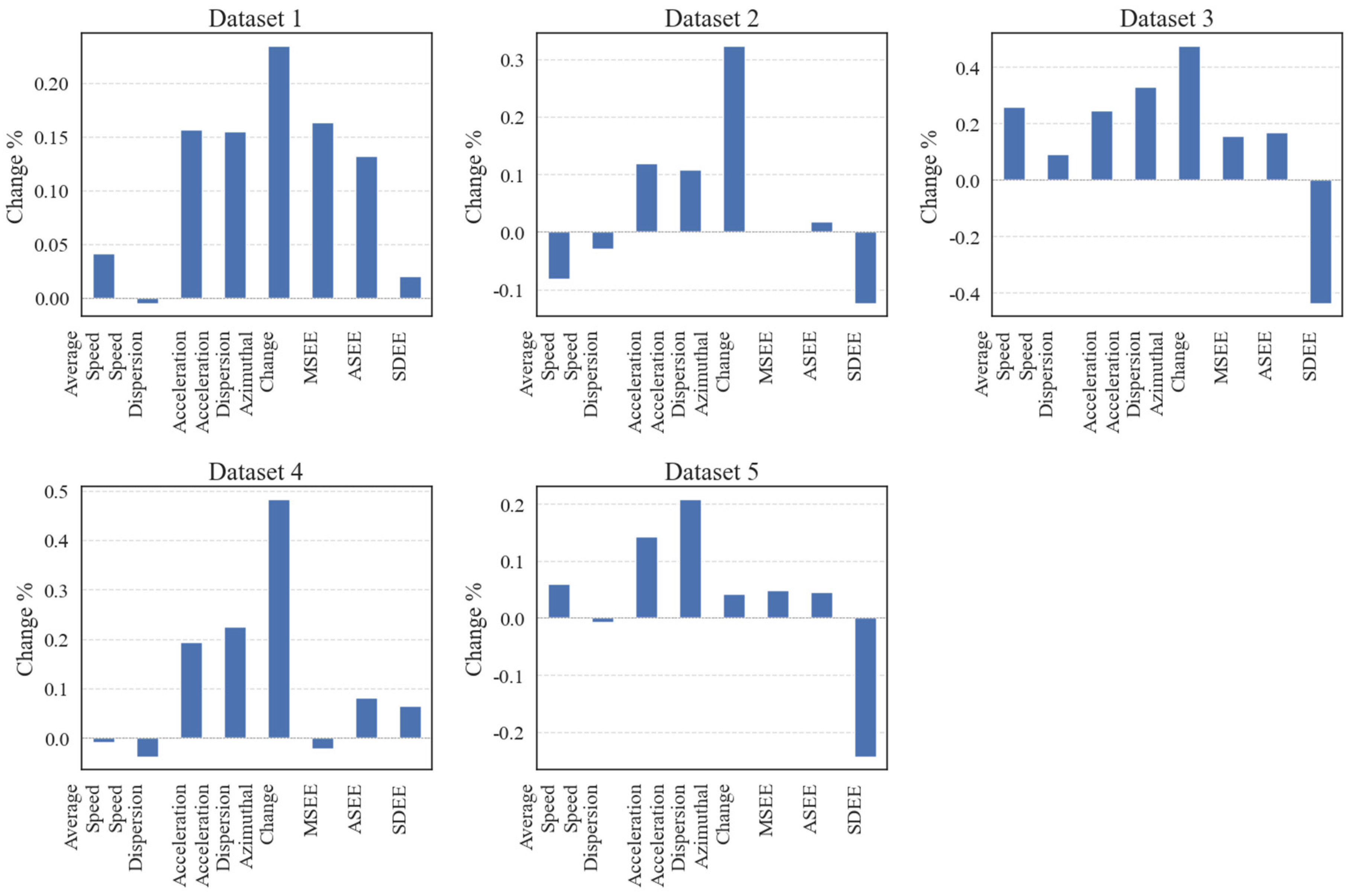
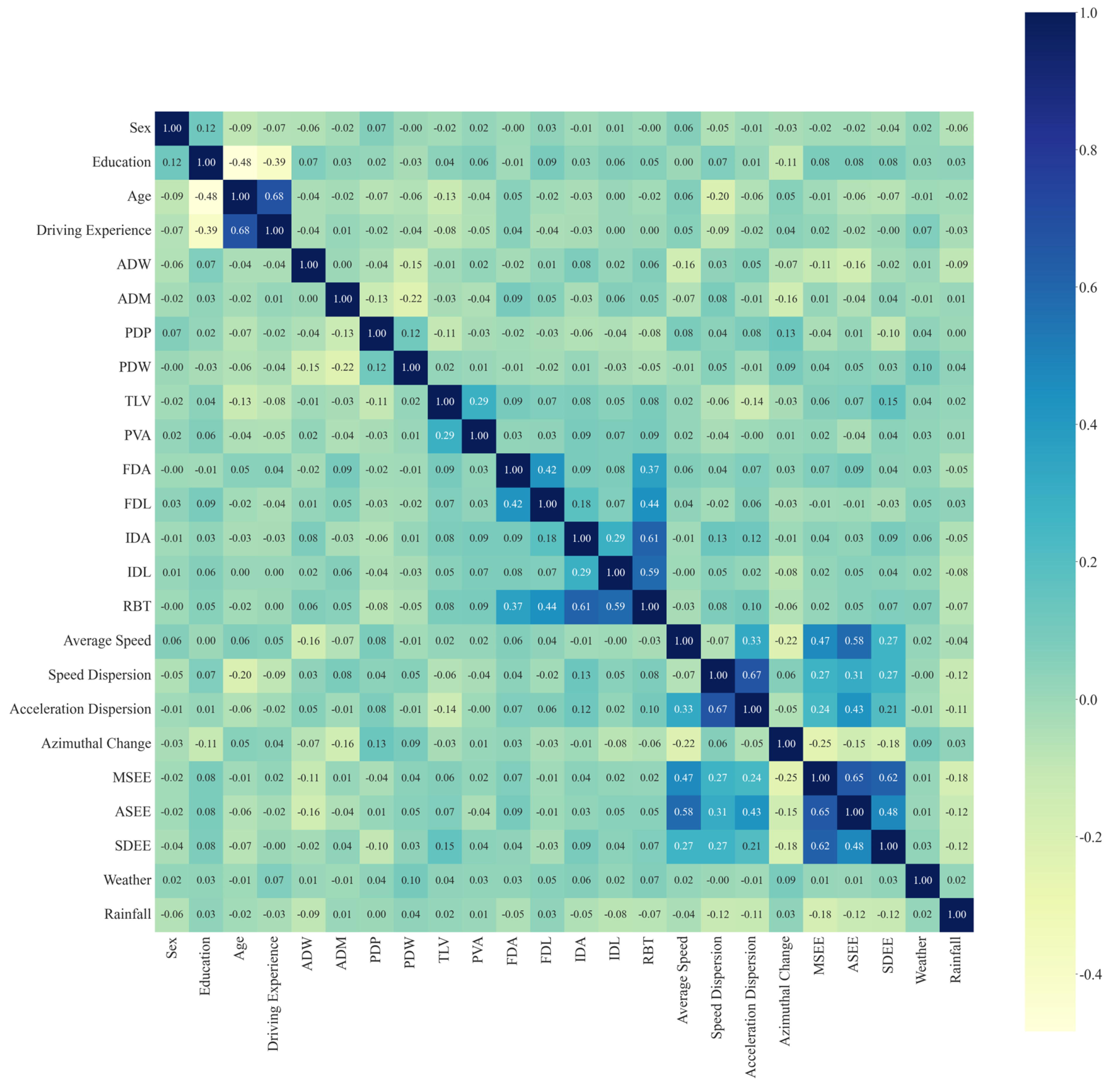

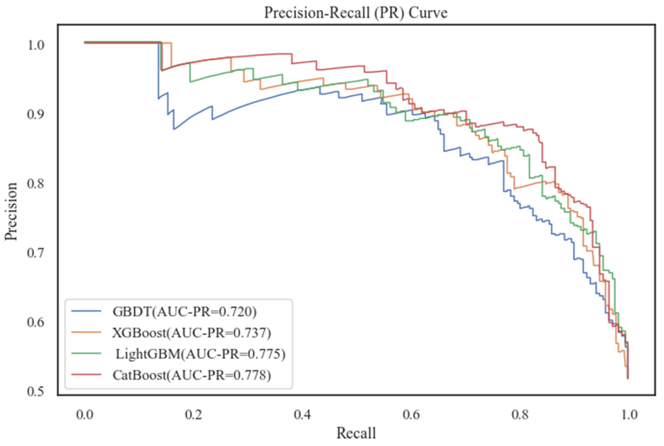
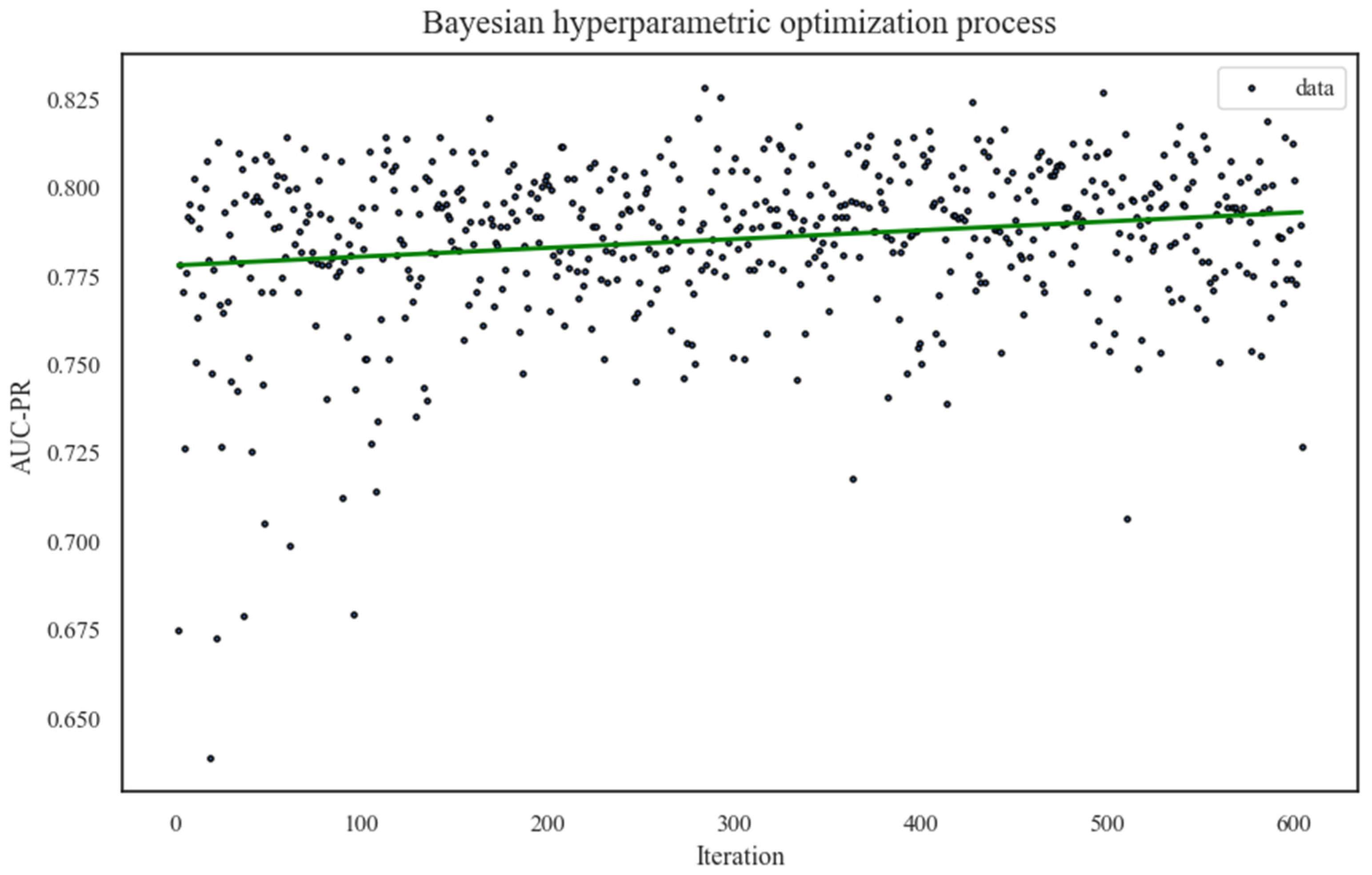
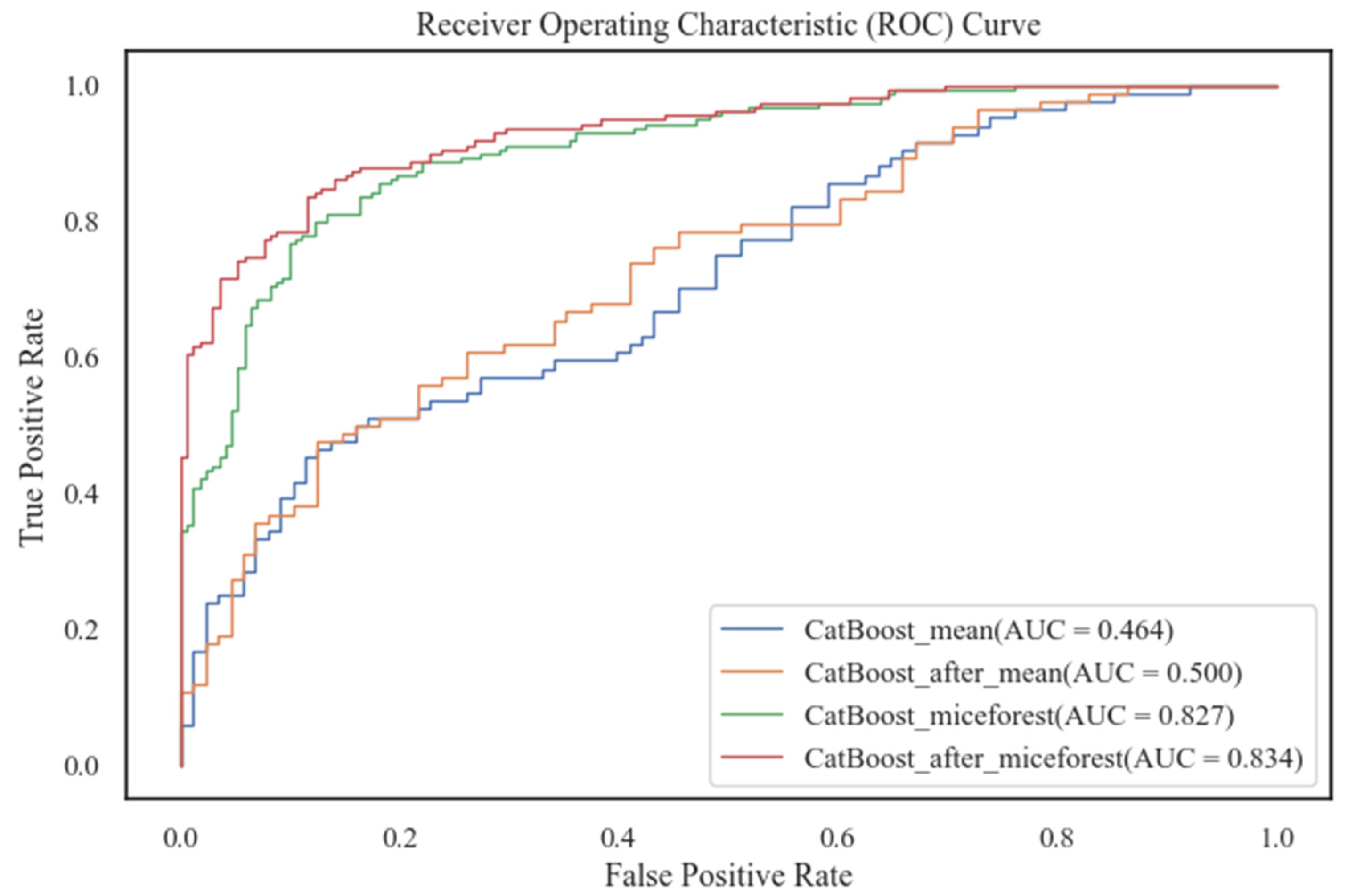
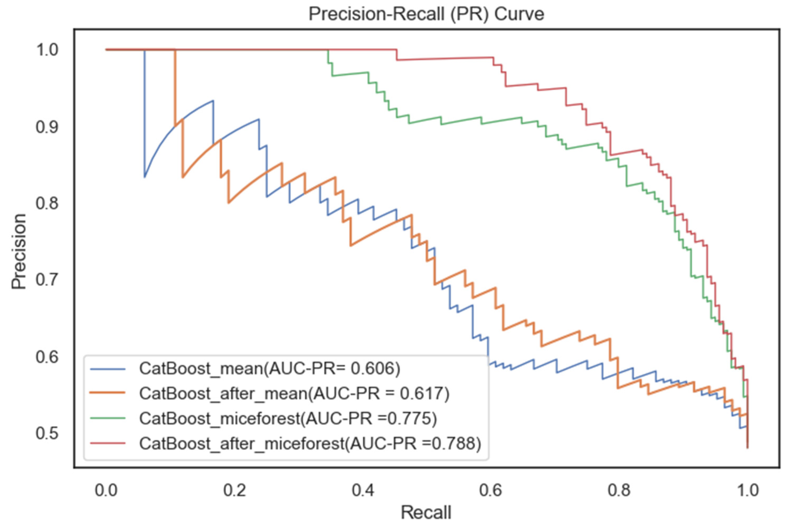
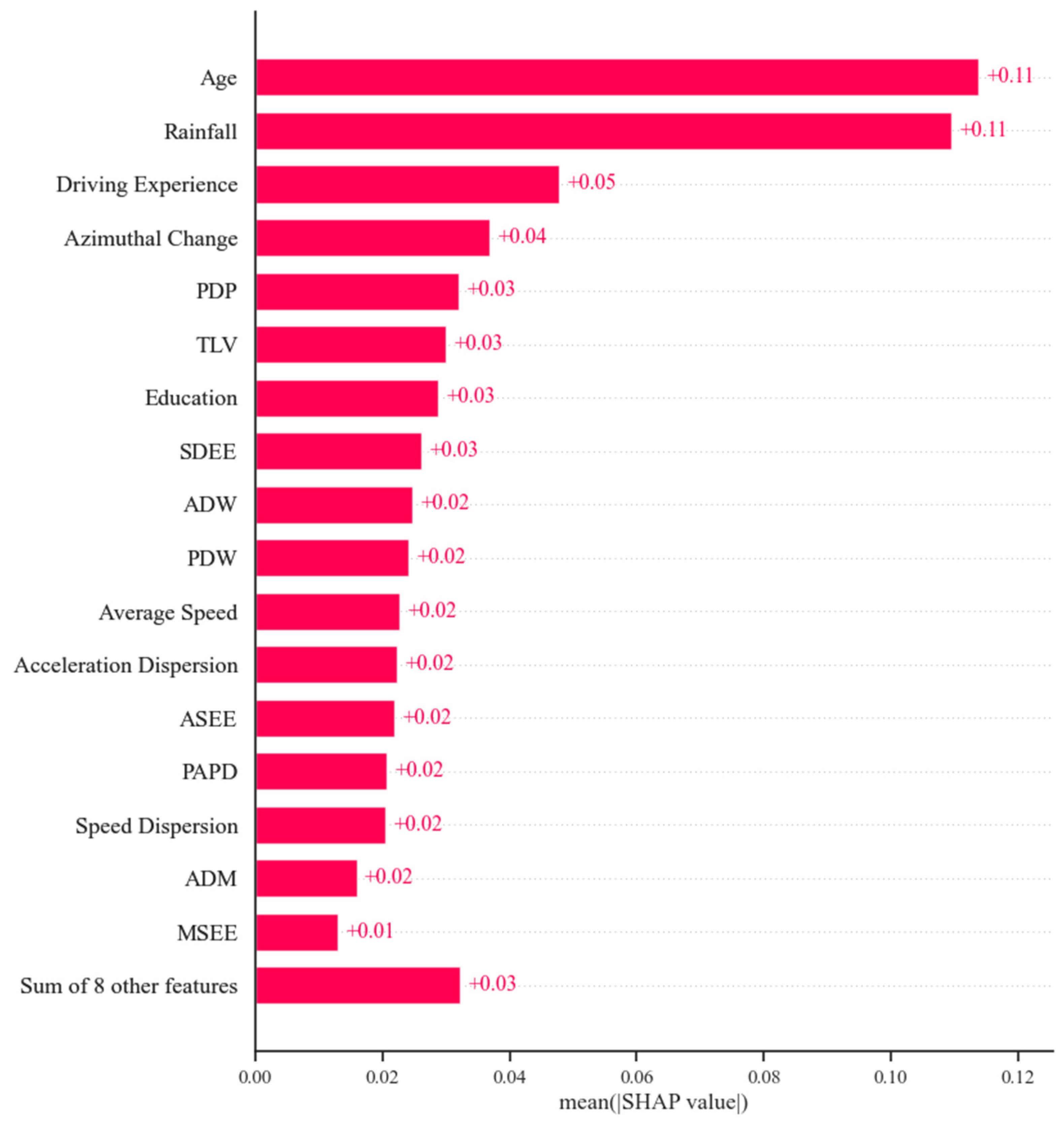
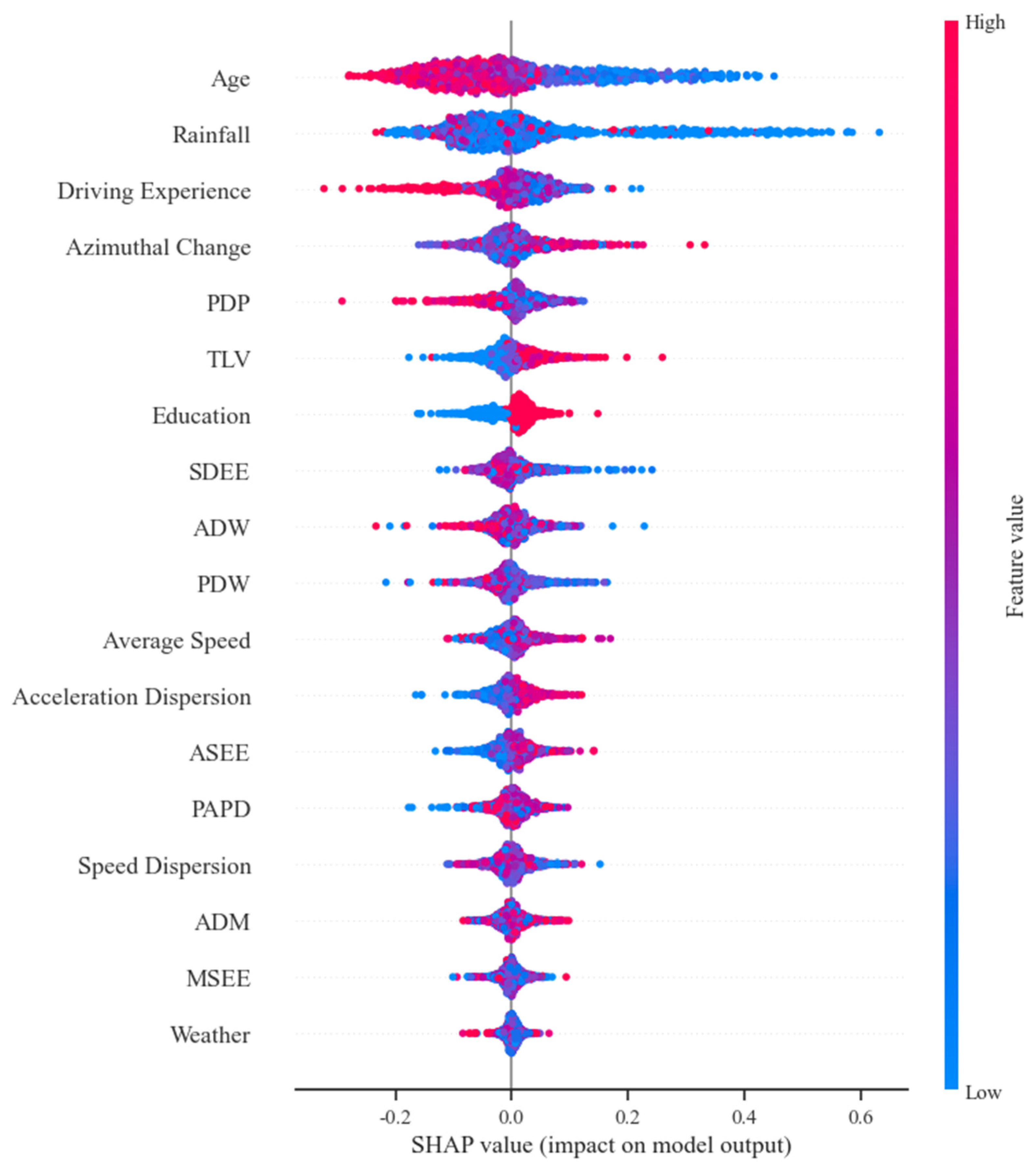

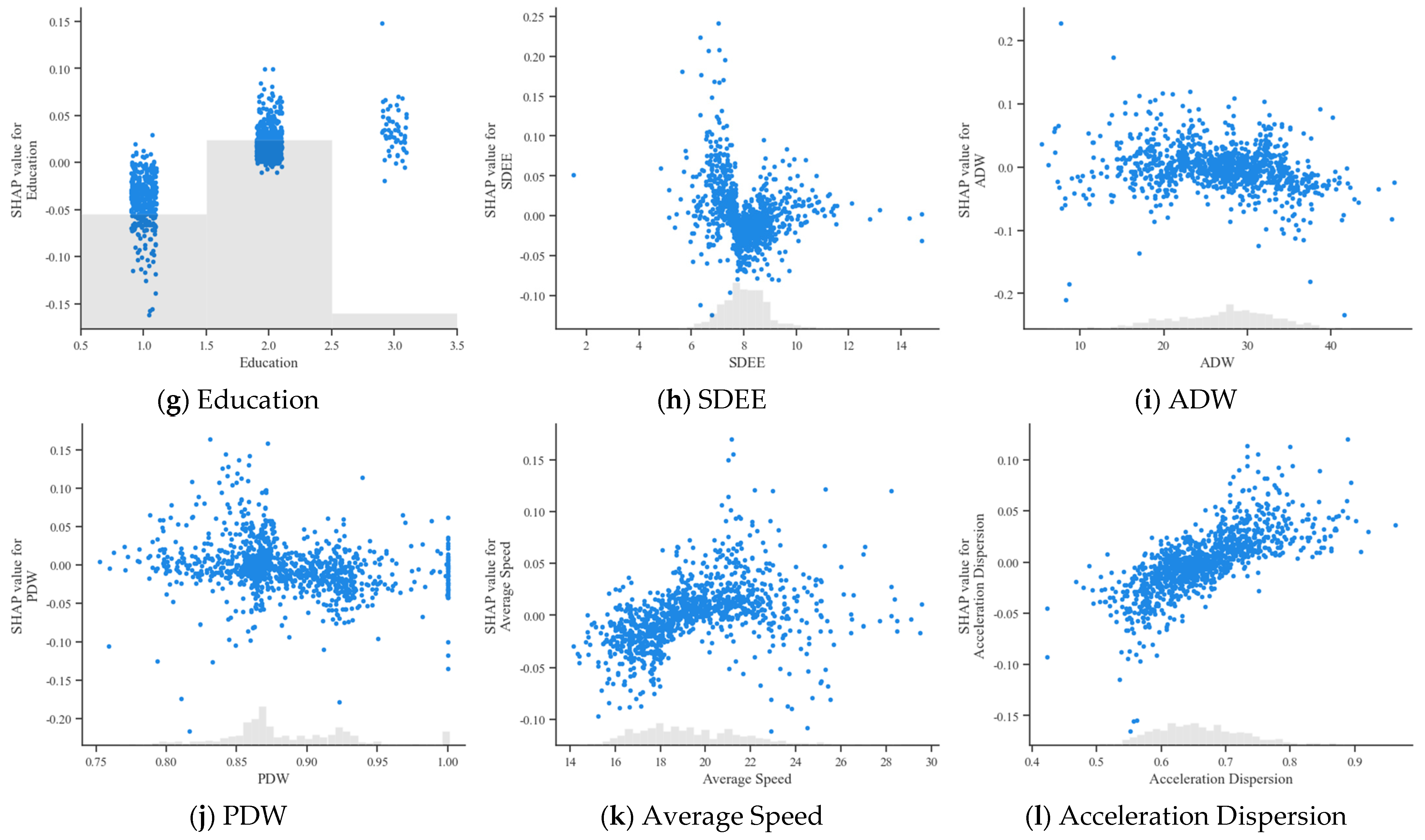
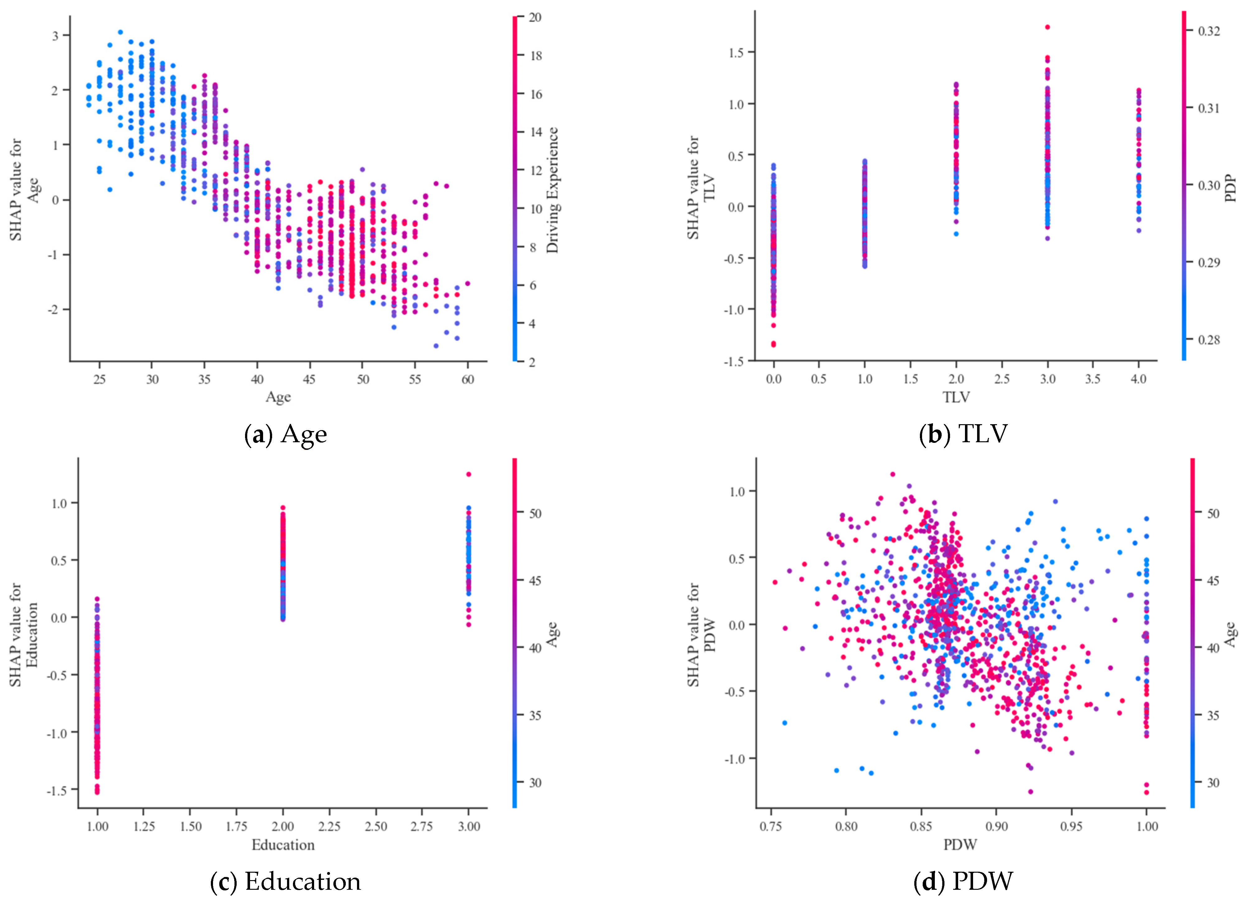
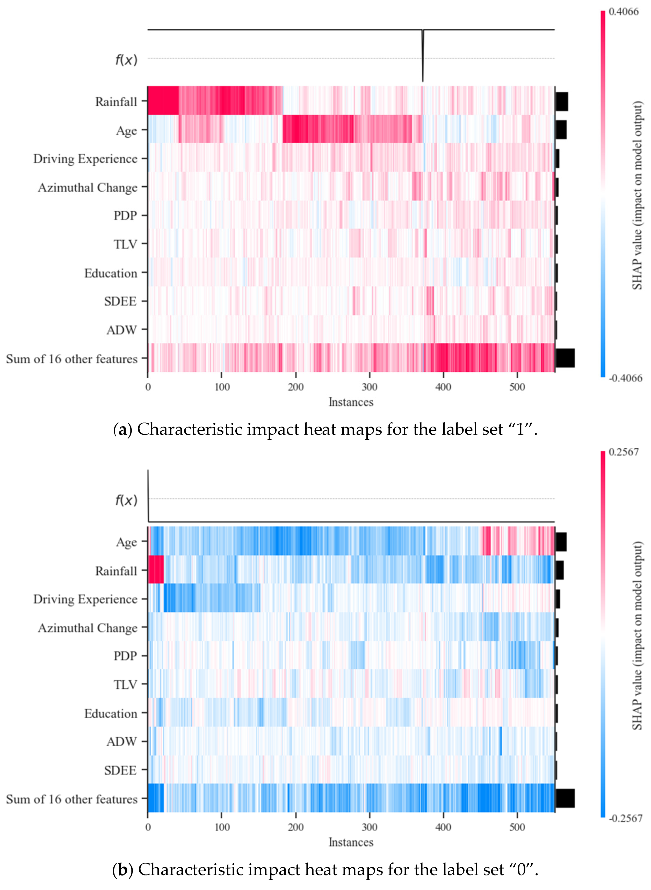
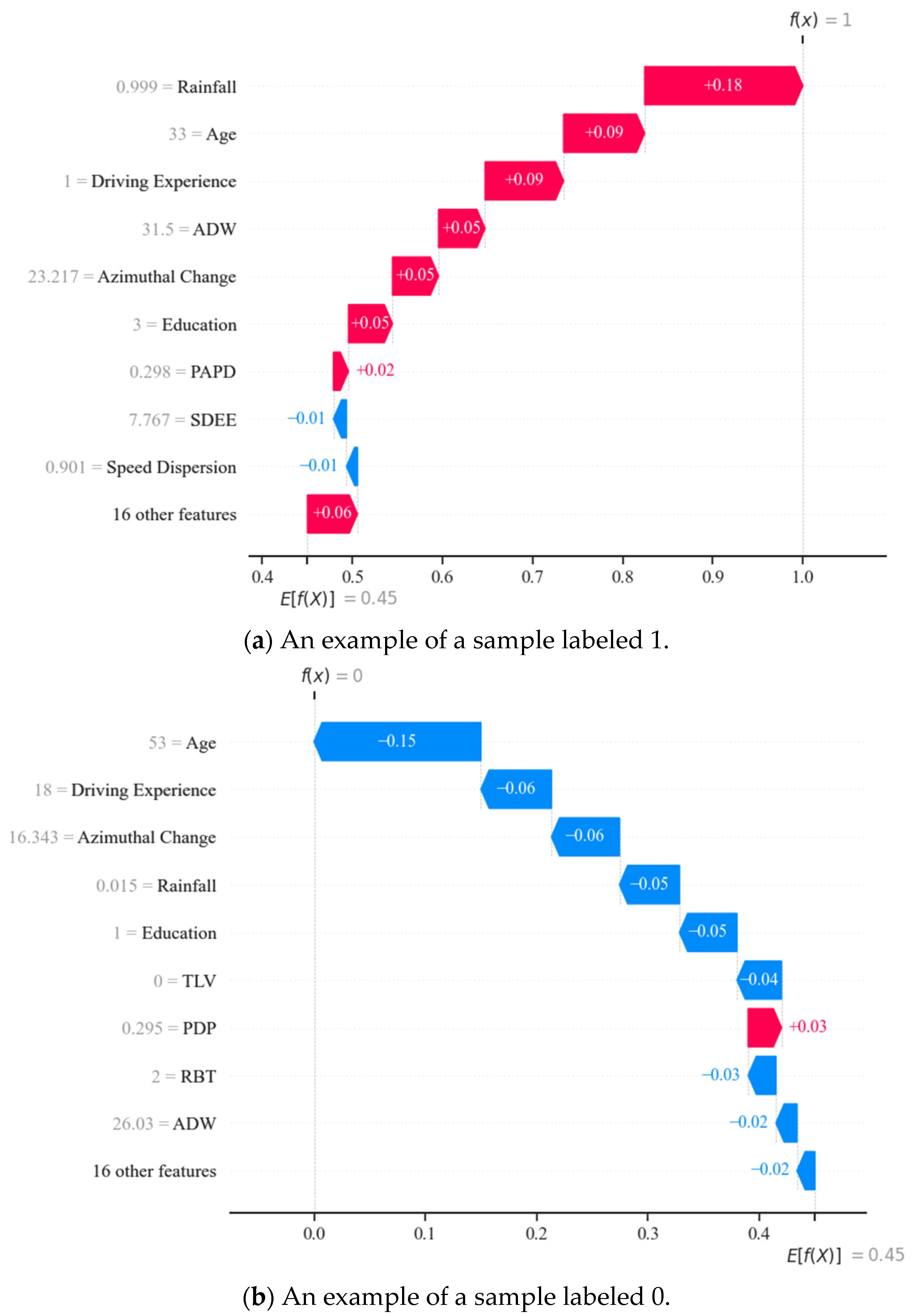
Disclaimer/Publisher’s Note: The statements, opinions and data contained in all publications are solely those of the individual author(s) and contributor(s) and not of MDPI and/or the editor(s). MDPI and/or the editor(s) disclaim responsibility for any injury to people or property resulting from any ideas, methods, instructions or products referred to in the content. |
© 2023 by the authors. Licensee MDPI, Basel, Switzerland. This article is an open access article distributed under the terms and conditions of the Creative Commons Attribution (CC BY) license (https://creativecommons.org/licenses/by/4.0/).