An Improved Contact Force Model of Polyhedral Elements for the Discrete Element Method

Abstract

The discrete element method (DEM) serves as a robust tool for simulating the mechanical behavior of granular materials. The accuracy of the DEM simulation is determined by the calculation of contact forces between elements. Compared to spherical elements, the contact modes of polyhedral elements are more complex. In this work, the contact force between polyhedral elements under different contact modes was investigated by experiment. Based on the experimental results, the normal stiffness coefficient in the Cundall’s contact model was modified. The improved contact force model was then applied in the DEM simulation and validated by means of comparison with the results of packing experiments. The research results demonstrate that the improved contact force model can be effectively applied to the simulation of different contact modes between polyhedral elements. The results of the packing experiment highly coincide with the results of the DEM simulation, which confirms the accuracy and reliability of the improved contact force model.

1. Introduction

Granular materials refer to a collection of discrete solid particles characterized by individual shapes, sizes, and interaction features. Various substances constitute granular materials, including sand, soil, powders, grains, and even small stones. They are among the most commonly encountered materials in natural environments, engineering applications, and daily life [1]. Therefore, granular materials are closely related to our lives and production. Studying the dynamic behavior of granular materials has always been an important research topic [2,3]. For example, the stability of earth–rock dams under external loads [4], the problem of slope hazards [5], and the fragmentation of railway ballast under the pulsation of trains all involve the dynamic behavior of granular materials [6].

Compared to continuous media, granular materials exhibit non-uniformity and anisotropy [7]. It is unsatisfactory to solve relevant engineering problems using the theory of continuous media. Therefore, non-continuous mechanics methods have been introduced, including discontinuous deformation analysis (DDA) [8,9], the finite–discrete element coupling method (FDEM) [10,11], the manifold method (NMM) [12], the material point method (MPM) [13,14], and the discrete element method (DEM) proposed by Cundall [15]. In the calculation of DEM, the analysis of the contact interaction between two particles is divided into two steps. The first step is usually called contact detection, which calculates the geometric features of overlap between two particles, including contact points, contact normal directions, contact depth, or contact volume. The second step is to calculate the contact force based on the geometric features of contact. DEM is further divided into particle-based DEM and block-based DEM. The main shape elements of particle-based DEM are discs and spherical particles, and the contact between particles is relatively simple [16]. The shape elements of block-based DEM are mainly polyhedrons, and the contact modes include point–point contact, point–edge contact, point–face contact, edge–edge contact, edge–face contact, and face–face contact [17,18]. Therefore, compared with particle-based DEM, the complexity of contact modes for polyhedral elements increases the difficulty of contact detection and contact force calculation [19].

Regarding the interaction between two particles, theoretical calculation methods for the contact force between particles have been proposed. Cundall proposed a block-based DEM model that regards polyhedral elements as rigid bodies that are connected by virtual springs [20]. When subjected to loads, force is transmitted through the deformation of springs, and the contact force between elements is divided into normal contact force and tangential contact force, considering the effect of damping. Thornton et al. incorporated the surface adhesion force of elements and the elastic and plastic deformation generated during the loading process into their consideration based on the basic theory of contact mechanics and proposed the spring–dashpot model [21]. Munjiza added relevant calculation methods for potential functions in the finite–discrete element coupling algorithm. Similar to Cundall’s model, it is assumed that polyhedral elements can overlap, and the contact force is calculated by integrating the potential function over the outer surface of the overlap region [10]. Feng et al. applied the energy method to the calculation of contact force between 2D polygons. Based on the energy method, the corner–corner contact between polygons is considered the basic contact mode, and other contact modes are special cases of corner–corner contact, which can be extended from the contact force calculation formula of corner–corner contact [22,23]. Rojek et al. proposed a method for calculating contact forces that utilizes a discrete element model with contact forces equivalent to given macroscopic virgin stresses [24]. In addition, experimental studies on the contact behavior between particles have been conducted. Hirofumi et al. used a pendulum device to collide two steel balls in order to study the effect of the strain rate on ball impact, and they obtained the coefficient of restitution (COR) and contact duration through impact tests [25]. In order to obtain the contact law applicable to discrete element numerical calculations, Cole et al. conducted a series of contact experiments on spherical crystal fragments with a diameter of 14.72 mm using a micro-mechanical model [26]. Liu et al. conducted particle collision experiments with particles of different shapes and contact types to study the contact behavior between particles and proposed a particle contact detection algorithm based on the principle of energy conservation [21]. Ouyang et al. investigated the relationship between micro parameters such as contact force in DEM simulations and the macro parameters of specimens by conducting uniaxial compression tests and direct tension tests [27]. Liu et al. designed a series of experiments to determine the sliding friction coefficients between particles with different shapes and contact forms, which improved the accuracy of calculating tangential contact forces between particles [28].

Unlike spherical particles, the contact forces of which can accurately be calculated based on simple contact depth using Hertz theory or other methods, the calculation of contact forces for non-spherical particles strongly depends not only on the overlapping area but also on the specific geometric configuration of the overlapping area [29]. Both of these factors are difficult to determine in numerical simulations, and the contact forces for different contact modes for polyhedral elements are still widely debated issues. Therefore, the mathematical relationship between the contact force and the contact overlap depth for polyhedral particles under different contact modes has not been well established.

In addressing these challenges, this study aims to establish a comprehensive understanding of the mathematical relationship between contact forces and contact overlap depth for polyhedral elements under different contact modes. By employing a combined approach of experimental investigation and numerical simulation, this work seeks to provide solutions to the difficulties posed by the unique geometric configurations of non-spherical particles in determining contact forces. Ultimately, this research endeavors to provide an improved contact force model and improve the accuracy of DEM simulations in polyhedron-based granular material systems.

In the following, this paper introduces an impact experimental method designed for polyhedral specimens in Section 2 in order to measure inter-element contact forces under different contact modes. Subsequently, in Section 3, based on Cundall’s contact model and utilizing experimental results, a stiffness correction coefficient is proposed, establishing the relationship between inter-element contact forces, stiffness, and contact depth under different contact modes. In Section 4, the improved contact force model is integrated into discrete element simulations, and the feasibility of the contact force model is validated by comparing contact forces for polyhedral elements under different contact modes in both experiments and simulations. In Section 5, three sets of packing experiments with cubic blocks of different sizes are designed. Using the DEM simulation based on the improved contact force model, these experiments are simulated to verify the accuracy of the contact force model and extend this approach to simulate granular materials composed of arbitrarily shaped polyhedral particles, demonstrating the feasibility of this method. Finally, in Section 6, a brief summary of the conclusions of this work is presented, and possible extensions are outlined.

2. Experimental Method

A series of experiments for measuring the contact force between polyhedral specimens under impact loading were proposed based on different contact modes. A self-designed force hammer loading device was used to apply impact force to polyhedral specimens. Thin-film pressure sensors were installed at the contact surface of the blocks to record the contact force between the polyhedral specimens, and strain gauges were used to record the deformation of the polyhedral specimens.

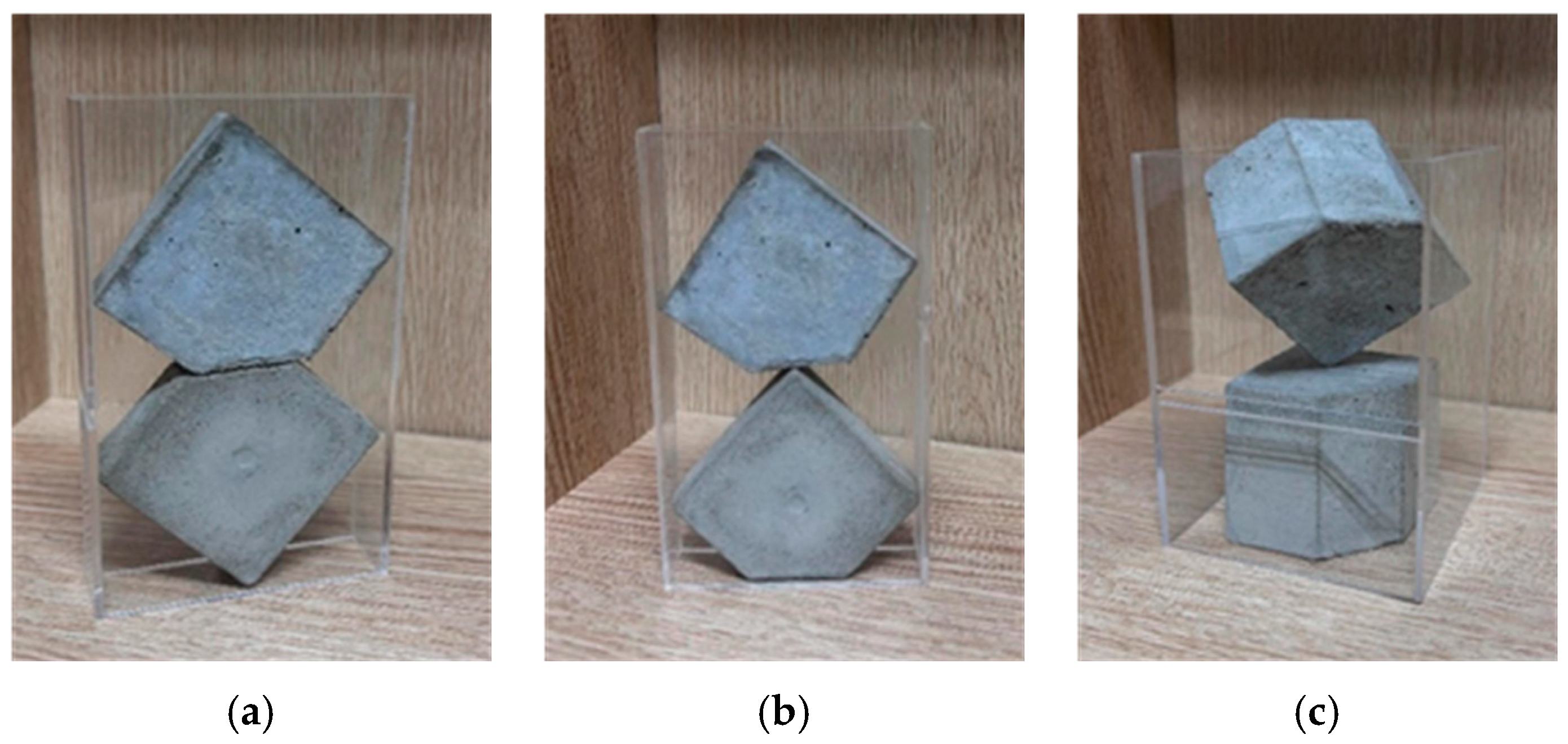
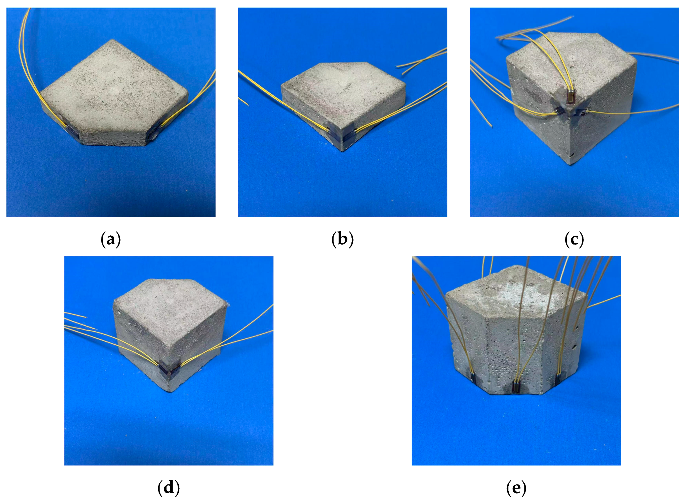
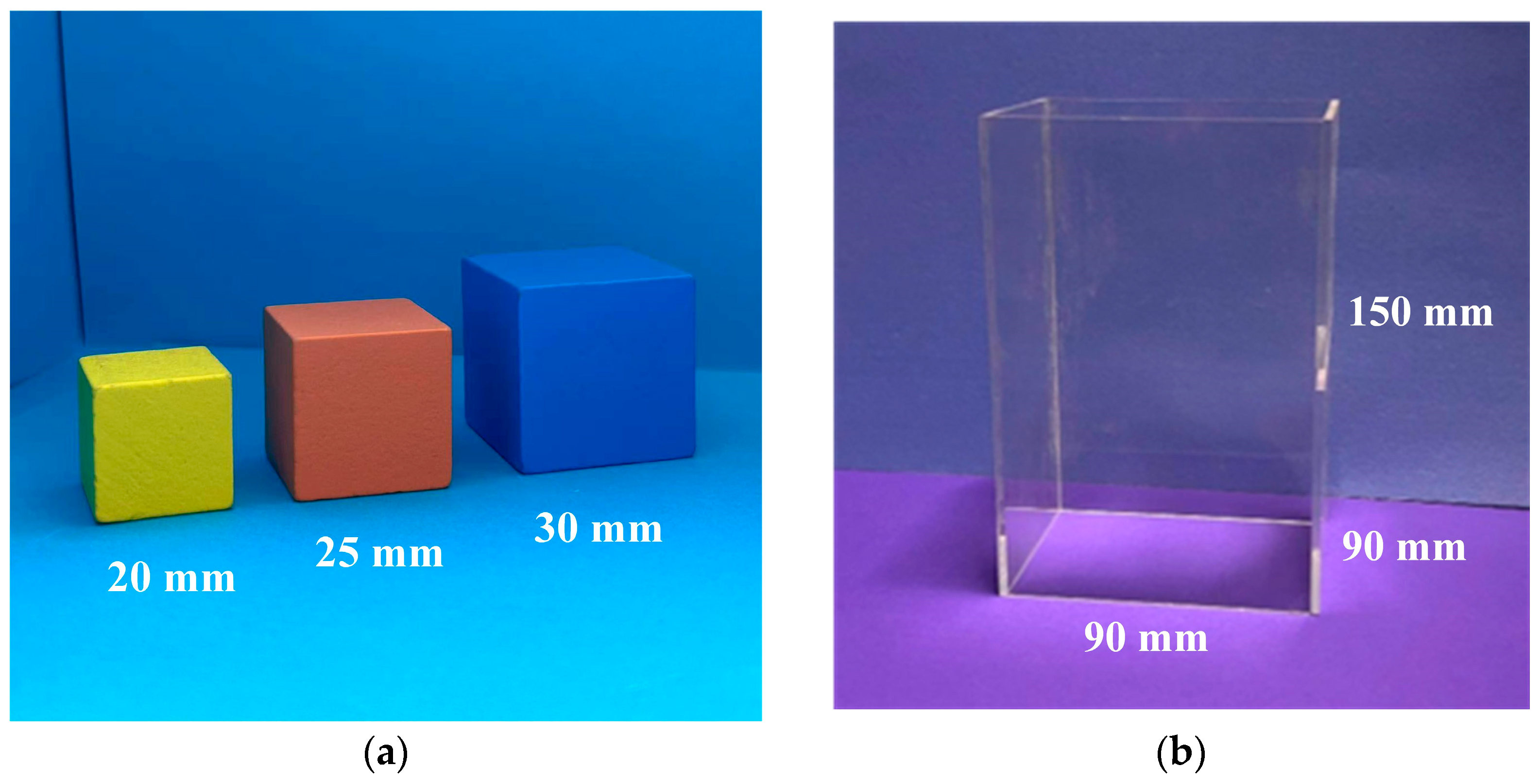
2.1. Design and Properties of Specimens

In order to facilitate the measurement of the contact force between specimens in the experiment and to take into account the range of the impact force hammer and the design of the fixing device, two types of cement mortar specimens were made, as shown in Figure 1. One corner of each block was cut at a 45-degree angle, 2 cm from one side.

The cement mortar specimens were prepared according to the mix ratio of cement/water/sand = 1:0.65:3, and sand with a particle size between 0.2 mm and 0.5 mm was selected as the fine aggregate. During the preparation of the cement mortar specimens, six rectangular cement mortar prisms with dimensions of 150 mm × 150 mm × 300 mm were manufactured. Following a standard curing period of 28 days, the compressive elastic modulus was measured for each specimen. The average elastic modulus of the six specimens in this experiment was determined to be 19.6 GPa. This average value was utilized in the calculation of the stiffness of the specimens.

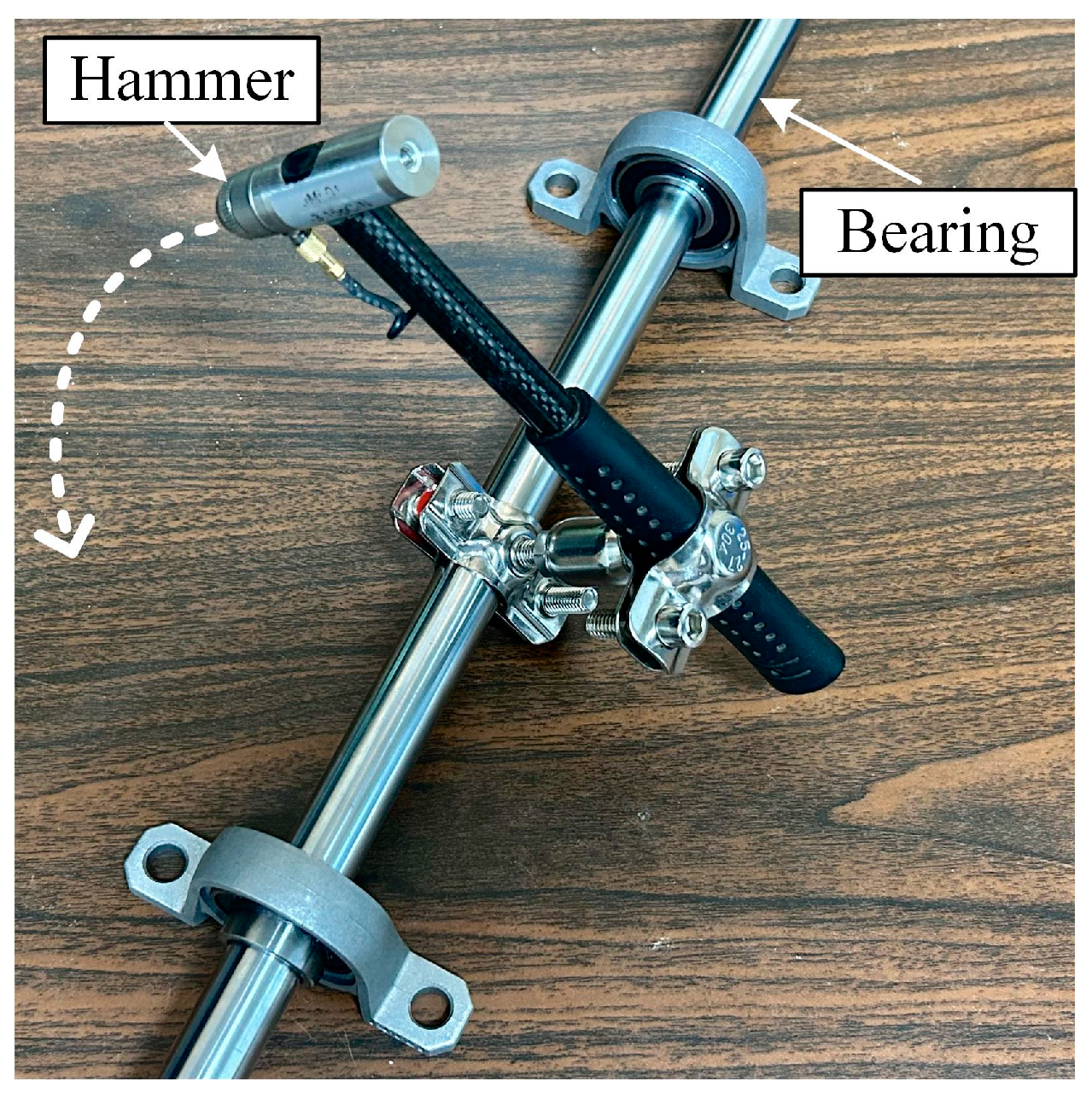
2.2. Experimental Equipment

The experimental equipment consisted of two parts: loading equipment and signal monitoring equipment. The commonly used impact force hammer in impact tests is usually applied by hand-held hammer handles, but this loading process in this manner is difficult to control. Therefore, in this work, a manually controlled impact force hammer loading device was designed, which mainly consisted of an impact force hammer, a signal converter, and a fixing device. The application of various levels of impact load was achieved by controlling the angle of the force hammer in the horizontal direction. The impact hammer used in this work is shown in Figure 2.

To monitor the contact force of different contact modes, three types of thin-film pressure sensors with different shapes were selected to cover the contact area of different contact modes. Circular thin-film pressure sensors with a diameter of 1 cm were used for point–edge contact, point–face contact, and edge–edge contact. The circular thin-film pressure sensor with a diameter of 3 cm was used for edge–face contact, and the square sensing area thin-film pressure sensor was used for face–face contact. In the discrete element method, the contact depth is often used as the independent variable to calculate the contact force. However, in the real situation, there is no overlap between the specimens. Therefore, the normal deformation between the specimens under the impact load was approximated as the contact depth, and strain gauges were used to calculate the normal direction of the contact depth between the blocks. The signals from the above two sensors were converted into voltage signals by a converter and transmitted to a dynamic signal acquisition instrument and a computer. The connection between the experimental equipment is shown as Figure 3.

2.3. Experimental Procedure

In this work, cement mortar specimens with thicknesses of 2 cm and 6 cm were prepared, and different contact modes were designed. Point–edge contact and edge–edge (collinear) contact were studied using blocks with a thickness of 2 cm (Figure 4a,b), while the remaining four contact modes were studied using blocks with a thickness of 6 cm (Figure 4c–f).

The specific process of this experiment was as follows:

(1)

The upper specimen was struck by controlling the angle of the impact force hammer, and the force was transmitted to the contact surface between the specimens through the compression caused by the impact.

(2)

When impacted, the pressure sensor on the impact force hammer generated a charge signal, which was converted into a voltage signal by the signal converter. The thin-film pressure sensor generated a corresponding current signal when sensing pressure, which was converted into a voltage signal by a linear voltage conversion module. The strain gauge changed its resistance due to deformation, and the signal amplifier converted it into a voltage signal. These three sets of signals were transmitted to the dynamic signal acquisition instrument.

(3)

The dynamic signal acquisition instrument transmitted the data to the dynamic signal testing and analysis software on the PC through a network cable, and generated data waveforms collected by the force hammer pressure sensor, thin-film pressure sensor, and strain gauge, thereby obtaining the time–domain curve of the impact force of the force hammer, the contact force between the blocks, and the strain curve.

2.4. Magnitude of Impact Force

To ensure that the block specimen did not experience significant displacement or breakage during the hammering process, nine different sizes of impact loads were used in the experiments. In the impact test, the loading of different sizes of impact force was achieved by manually controlling the angle between the hammer and the horizontal plane. The magnitude of the impact force in the experiments of different contact types, as measured by the hammer sensor, is shown in

Table 1. Magnitude of impact force for different contact modes (N).

Group	Edge–Edge (Collinear)	Point–Edge	Point–Face	Edge–Edge (Non-Collinear)	Edge–Face	Face–Face
1	65.31	68.60	69.84	69.10	80.42	62.81
2	72.28	70.14	71.26	70.35	83.64	68.11
3	78.18	73.53	74.20	72.49	87.37	73.58
4	111.14	114.52	117.18	115.49	115.21	120.73
5	115.79	118.85	121.55	118.68	118.96	124.65
6	121.82	125.21	122.59	123.01	123.51	127.09
7	176.68	165.72	165.82	149.46	166.90	172.87
8	177.35	169.34	168.69	155.23	170.21	173.62
9	179.68	175.09	173.92	160.57	174.86	176.82

.

3. Calculation of Contact Force

The contact model proposed by Cundall includes two parameters typically utilized for calculating contact forces between spheres, as shown in Equation (1).

$$F_n=k_n\times \delta$$

(1)

where $\delta$ represents the contact depth and $k_n$ represents the stiffness coefficient. The contact depth is calculated by the contact detection algorithm, so the normal stiffness coefficient determines the accuracy of the contact force calculation. Unlike spherical elements, there are various contact modes among polyhedral elements, which may result in Equation (1) being inapplicable in all contact modes. Therefore, a method based on impact experiments is proposed in this section to determine the stiffness correction factor, and Equation (1) is modified for different contact modes of the polyhedral elements.

3.1. Contact Depth

In the discrete element method, the element is assumed to be a rigid body. When the polyhedral element is subjected to external forces, begins to move, and comes into contact with adjacent elements, the two contacting polyhedral elements are allowed to overlap, and the depth of the overlap is called the contact depth.

In Cundall’s spring-damping model, it is assumed that there is a spring between the elements, which shortens when the two elements are compressed. The compression of the spring is the contact depth, and the magnitude of the contact force between the elements is also characterized by it. In reality, when two specimens are subjected to an impact load, damage may occur, and there is no overlap, so the contact depth cannot be directly measured. Therefore, strain gauges were attached to the specimens to measure the strain values near the contact point, edge, or face, and the estimated contact depth was obtained through vector calculations. The positions of the strain gauges attached to the specimens’ contact surface under different contact modes are shown in Figure 5, where the positions of the strain gauges attached to the edge–edge contact and edge–face contact are the same.

As an example, the calculation of the contact depth for edge–face contact is shown in the schematic diagram in Figure 6. ${\epsilon }_1$ and ${\epsilon }_2$ in the figure are strain vectors measured by strain gauges, and the normal strain vector $\epsilon$ is obtained by vector addition of ${\epsilon }_1$ and ${\epsilon }_2$ using the parallelogram law. The estimated contact depth can be obtained using Equation (2):

$$\delta =\epsilon \times L$$

(2)

where L is the length of the specimen in the normal direction. The calculated contact depths are shown in

Table 2. Contact depth for different contact modes (m).

Group	Edge–Edge (Collinear)	Point–Edge	Point–Face	Edge–Edge (Non-Collinear)	Edge–Face	Face–Face
1	−9.1 × 10−8	−8.4 × 10−8	−6.1 × 10−8	−6.9 × 10−8	−8.6 × 10−8	−7.2 × 10−8
2	−9.1 × 10−8	−7 × 10−8	−5.9 × 10−8	−7.3 × 10−8	−1 × 10−7	−7 × 10−8
3	−1 × 10−7	−9 × 10−8	−8.5 × 10−8	−6.7 × 10−8	−7.8 × 10−8	−7.8 × 10−8
4	−1.4 × 10−7	−9.7 × 10−8	−9.8 × 10−8	−9.6 × 10−8	−1.1 × 10−7	−1.4 × 10−7
5	−1.4 × 10−7	−1.1 × 10−7	−1.2 × 10−7	−8.2 × 10−8	−1 × 10−7	−1.2 × 10−7
6	−1.3 × 10−7	−1.2 × 10−7	−1.2 × 10−7	−1.1 × 10−7	−1.2 × 10−7	−1.2 × 10−7
7	−2 × 10−7	−1.5 × 10−7	−2.2 × 10−7	−1.4 × 10−7	−1.4 × 10−7	−1.4 × 10−7
8	−2.1 × 10−7	−1.4 × 10−7	−2 × 10−7	−1.2 × 10−7	−1.9 × 10−7	−1.8 × 10−7
9	−2.1 × 10−7	−1.6 × 10−7	−2.5 × 10−7	−1.5 × 10−7	−1.8 × 10−7	−1.8 × 10−7

.

3.2. Normal Stiffness

To correct the normal stiffness coefficient, a universally applicable initial value of the normal stiffness coefficient needs to be determined. Therefore, the formula for calculating the normal stiffness coefficient $k_n$ derived from the collision between a spherical ball and a plane in reference [30] is used in this work. The formula takes into account the elastic modulus and Poisson’s ratio of the material itself when calculating the contact force. The specific method for determining the normal stiffness coefficient is as follows:

$$k_n=\frac{4}{3}\frac{E}{(1-{\sigma }^2)}\sqrt{R}$$

(3)

where E represents the elastic modulus of the material, $\sigma$ represents the Poisson’s ratio, and R represents the radius of the equivalent sphere.

Since there are two different thicknesses of the specimens used in this experiment, substituting the values yields an equivalent sphere radius of 2.5325 × 10⁻² m for the specimen with a thickness of 2 cm and an equivalent sphere radius of 3.6525 × 10⁻² m for the specimen with a thickness of 6 cm. After substituting the equivalent sphere radius into Equation (3), the normal stiffness coefficients for the two types of specimens are 1.5234 × 10⁹ N/m and 1.8295 × 10⁹ N/m, respectively.

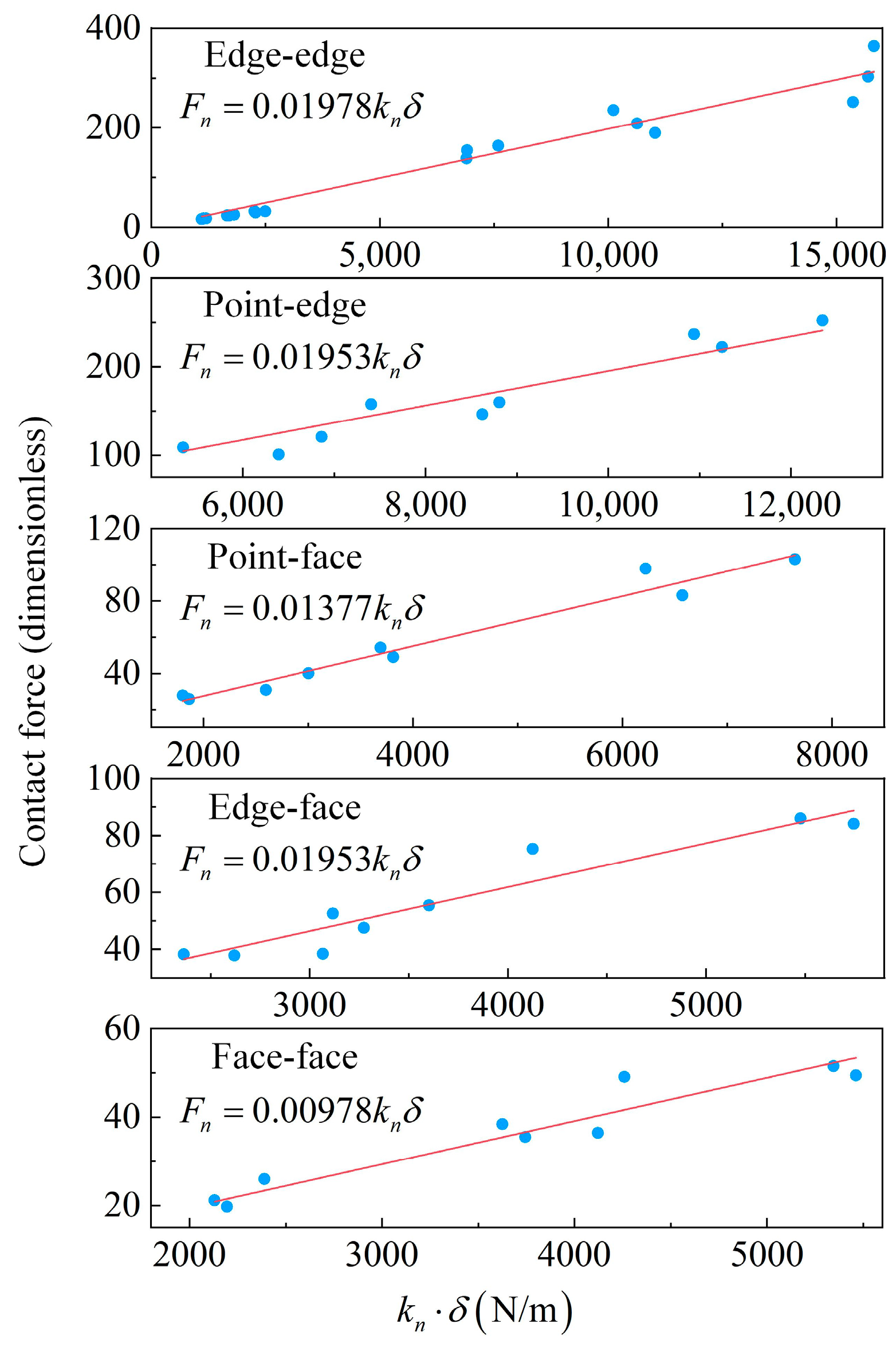
3.3. Stiffness Correction Factor

In order to eliminate the influence caused by the difference in specimen thickness in edge-to-edge contact, both co-linear and non-co-linear edge-to-edge contacts were considered as the same type of contact when revising the initial normal stiffness coefficient values. Therefore, the contact depth and contact force were dimensionless by normalizing them. Firstly, the ratio of the contact depth to the corresponding thickness for each type of contact was used as the dimensionless contact depth. Secondly, the ratio of the contact force peak to the corresponding block weight for each type of contact was used as the dimensionless contact force amplitude.

Based on the dimensionless contact depth and contact force, a linear fitting method was used to revise the initial normal stiffness coefficient values. In the fitting of the contact force formula, x is the product of $k_n$, $\delta$ is the dimensionless contact depth, and y is the dimensionless contact force amplitude. The linear fitting function was used to fit the contact force formula for each type of contact of specimens, with the intercept set to zero.

Figure 7 shows the fitting results of the initial normal stiffness coefficient values based on dimensionless experimental data for different contact modes. The R² values of the fitting curves for each contact mode are 0.98084, 0.99085, 0.99174, 0.99048, and 0.99083, respectively. The effectiveness of linear fitting is determined by the variance of the fitting curve calculated by R², with a value closer to 1 indicating a better fitting. The R² values of the fitting curves for all five types of contact are above 0.98, indicating a good fitting degree. The coefficients preceding k_n in the equations in the figures are the stiffness correction coefficients for different contact modes.

4. Comparison between DEM and Experimental Results

The improved contact force model was then embedded into the DEM code, which consists of four main parts: initial configuration, contact detection, contact force calculation, and updating of the particle motion status. The specific calculation flow chart is shown in Figure 8.

The measured impact force–time curve was selected as the input load, and the motion process of the polyhedral specimen under six different contact modes was simulated by the designed DEM program. The contact force–time curves obtained by simulation under different contact modes were compared and analyzed with the experiment.

4.1. Two Elements under Edge–Edge Contact Mode

4.1.1. Collinear

From Figure 9, it can be seen that the trend of the simulated contact force–time curve is roughly consistent with the curve in the experiment, and the opening size and amplitude of the main peak are close. However, the contact force–time curve obtained by the discrete element simulation is shifted upward compared to the experiment—that is, there is no negative value. This is because in the simulation, when the upper specimen is subjected to an impact load, it produces a slight vition, and when it separates from the lower specimen, the contact force returns to zero. In the experiment, the contact force is measured by a thin-film pressure sensor, although the blocks no longer contact each other due to the vition, and the thin-film pressure sensor produces a certain restoring force to restore deformation, resulting in negative values in the experiment. The relative error between the peak contact force obtained by the discrete element simulation and the experimental value is within 3%.

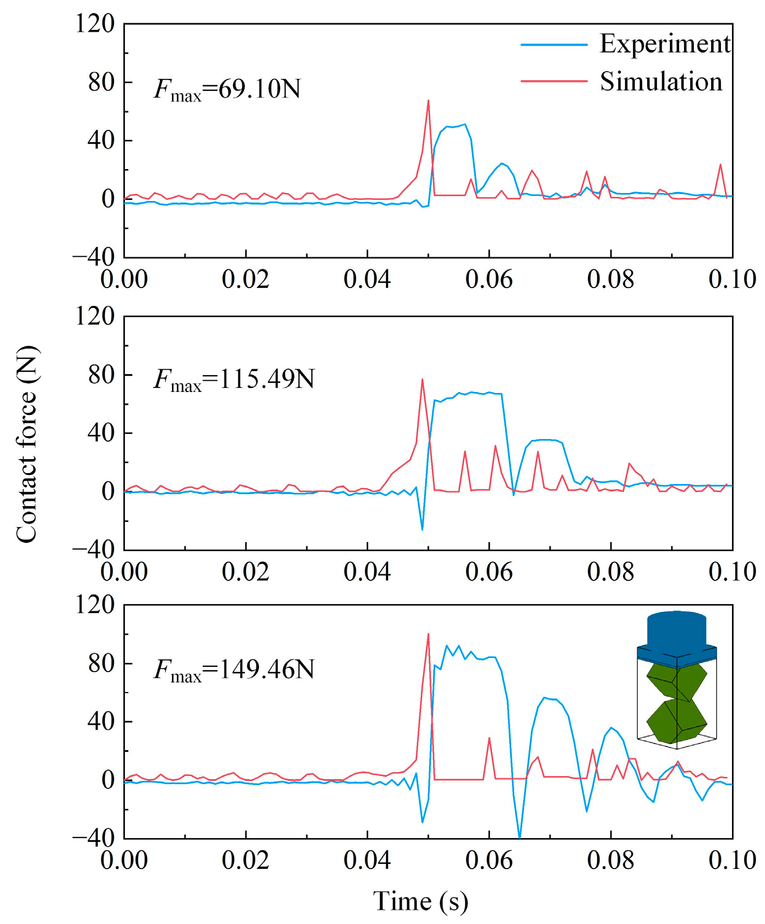
4.1.2. Non-Collinear

From Figure 10, it can be observed that the variation trend of the contact force–time curves obtained from simulation and experiment under different impact loads is roughly consistent, and the amplitude of the contact force is similar. The relative error between the peak contact force obtained from the discrete element simulation and the experimental value is within 14%. The experimental results in the figure exhibit a phenomenon of “anomalous waveform”. This is due to the non-collinear nature of the contact, where the contact form is an edge–edge contact. In reality, two polyhedra make contact at a single point. This type of contact poses significant challenges for the installation of thin-film pressure sensors. Improper installation may result in uneven force distribution on the sensor, consequently causing waveform anomalies.

4.2. Two Elements under Point–Edge Contact Mode

From Figure 11, it can be observed that under different loads, the opening size and amplitude of the main peak are similar, and the time of the small wave peak that appears after the first peak in the contact force–time curves obtained from simulation and experiment is also close, with a slight offset in the two curves after the peak. The relative error between the peak contact force obtained from the discrete element simulation and the experimental value is around 13%. The results obtained from the experiment indicate that, after time t = 0.05 s, the contact force does not stabilize near zero but continues to rapidly decrease until it reaches stability in the vicinity of a negative value. This is attributed to the elastic properties of the membrane material in the thin-film pressure sensor. Following the impact load, the membrane of the thin-film pressure sensor may undergo elastic deformation. Once the impact force dissipates, the membrane rebounds, generating a reverse force and causing the collected contact force by the sensor to stabilize near a negative value.

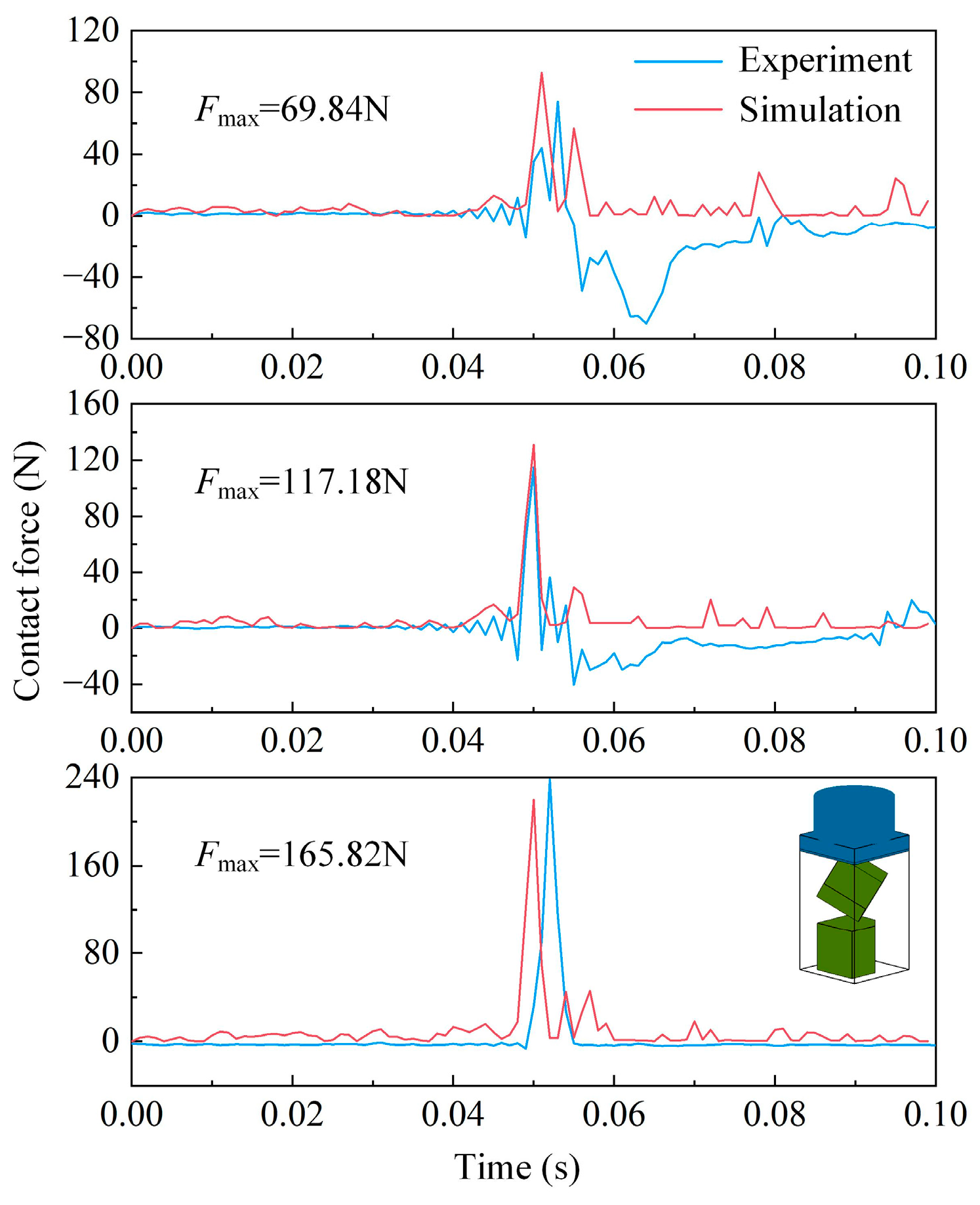
4.3. Two Elements under Point–Face Contact Mode

When the contact mode is point–face contact, the contact force–time curves obtained from simulation and experiment are consistent. Observing the contact force–time curves obtained from discrete element simulation and experiment in Figure 12, it can be found that the two curves become more consistent with the increase in impact load under this contact mode. The relative error between the peak contact force obtained from the experiment and that obtained from the discrete element simulation under this contact mode is around 15%.

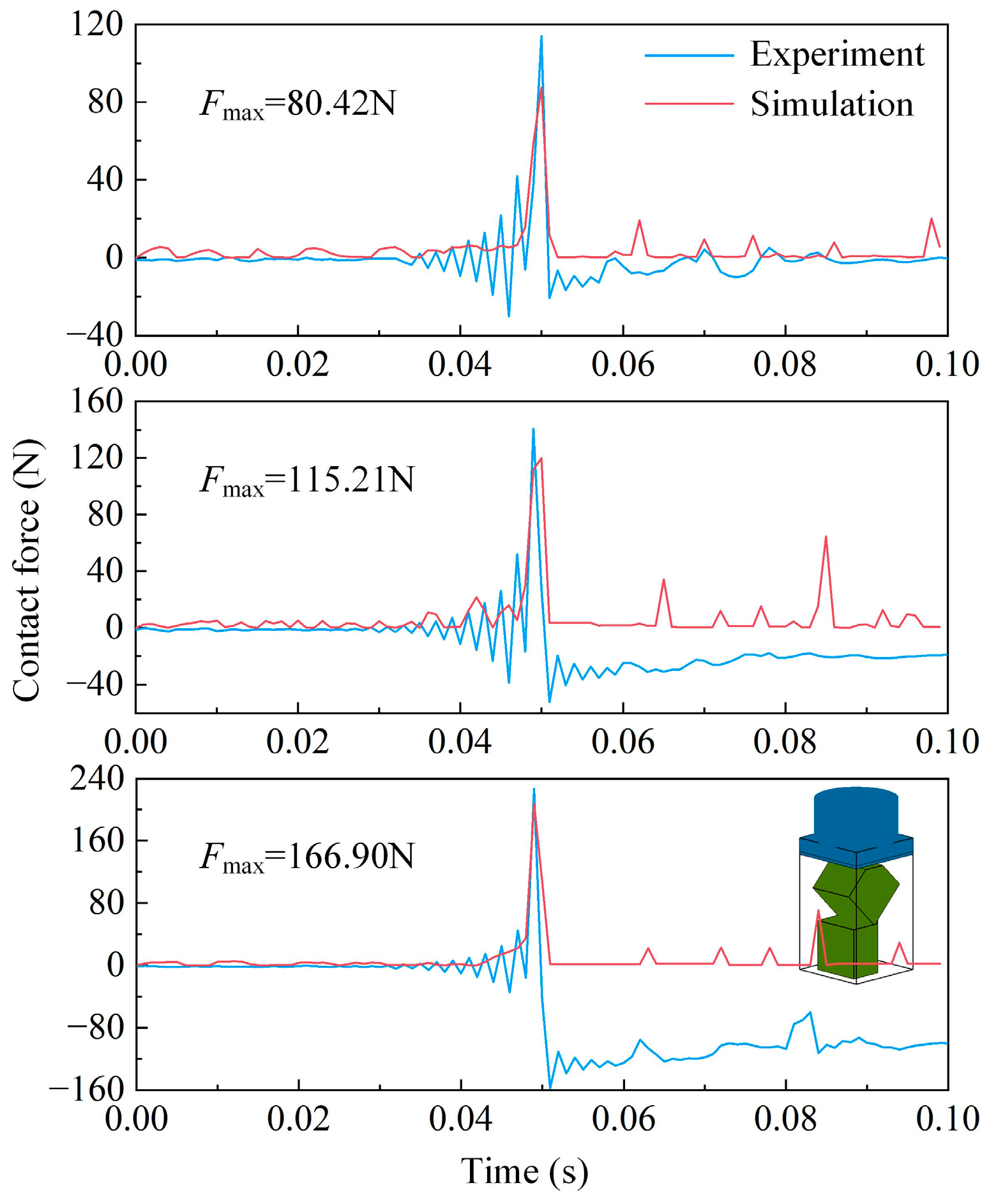
4.4. Two Elements under Edge–Face Contact Mode

From Figure 13, it can be observed that under different loads, the variation trend of the contact force–time curves obtained from the simulation and experiment is basically consistent, and the amplitude of the peak is similar. Similarly, in the unloading stage, there is an upward shift in the contact force–time curve obtained from the simulation relative to that obtained from the experiment. The relative error between the peak contact force obtained from the discrete element simulation and the experimental value under edge–face contact is around 13%. The phenomenon observed in Figure 13, where the contact force recorded by the sensor stabilizes near a negative value after reaching its peak, is consistent with the reasons discussed in Figure 11. This situation does not impact the normal functionality of the thin-film pressure sensor, and it remains capable of accurately capturing the peak contact force.

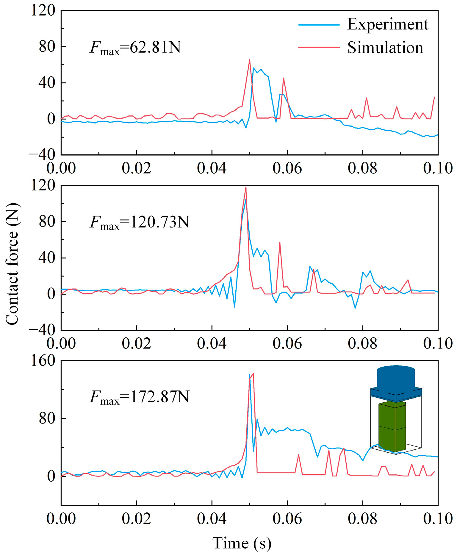
4.5. Two Elements under Face–Face Contact Mode

From Figure 14, it can be observed that the amplitude of the contact force peak obtained from simulation and experimental measurement is similar under different loading conditions, but the contact force–time curve obtained from simulation during the unloading stage is relatively smoother compared to the experimental measurement. This is because the specimen vibrates when it is subjected to an impact. Once the upper specimen separates from the lower block in the simulation, the contact force between the specimens becomes zero, whereas in the experiment, the contact force is not immediately reduced due to the sensitivity of the sensor. The relative error between the contact force peak obtained from the discrete element simulation and the experimental measurement under face–face contact is around 15%. The experimental results show that, after time t = 0.05 s, an overall waveform shift can be observed, and the waveform no longer stably oscillates around the zero value. The reason for this phenomenon is attributed to the instantaneous and high-energy input of the impact load. Under sufficiently high-energy conditions, it may lead to an unstable or uneven response in the thin-film pressure sensor. When the energy reaches a certain level, the instantaneous response can cause a waveform shift or drift after reaching the peak contact force. This situation does not affect the accurate capture of the peak contact force.

In the comparison of the simulation and experimental results of polyhedron unit contact forces under various contact modes mentioned above, we observed a small relative error in the maximum simulated contact force, and the simulated contact force exhibited a pattern similar to the experimental results. This suggests that a certain level of accuracy in simulation is achieved by the improved contact force model. To further substantiate the effectiveness of the improved contact force model, a series of packing experiments with cubic blocks were conducted in the subsequent section, and a comprehensive comparison was made between the experimental results and the simulations, both before and after the improvement.

5. Verification of Simulation

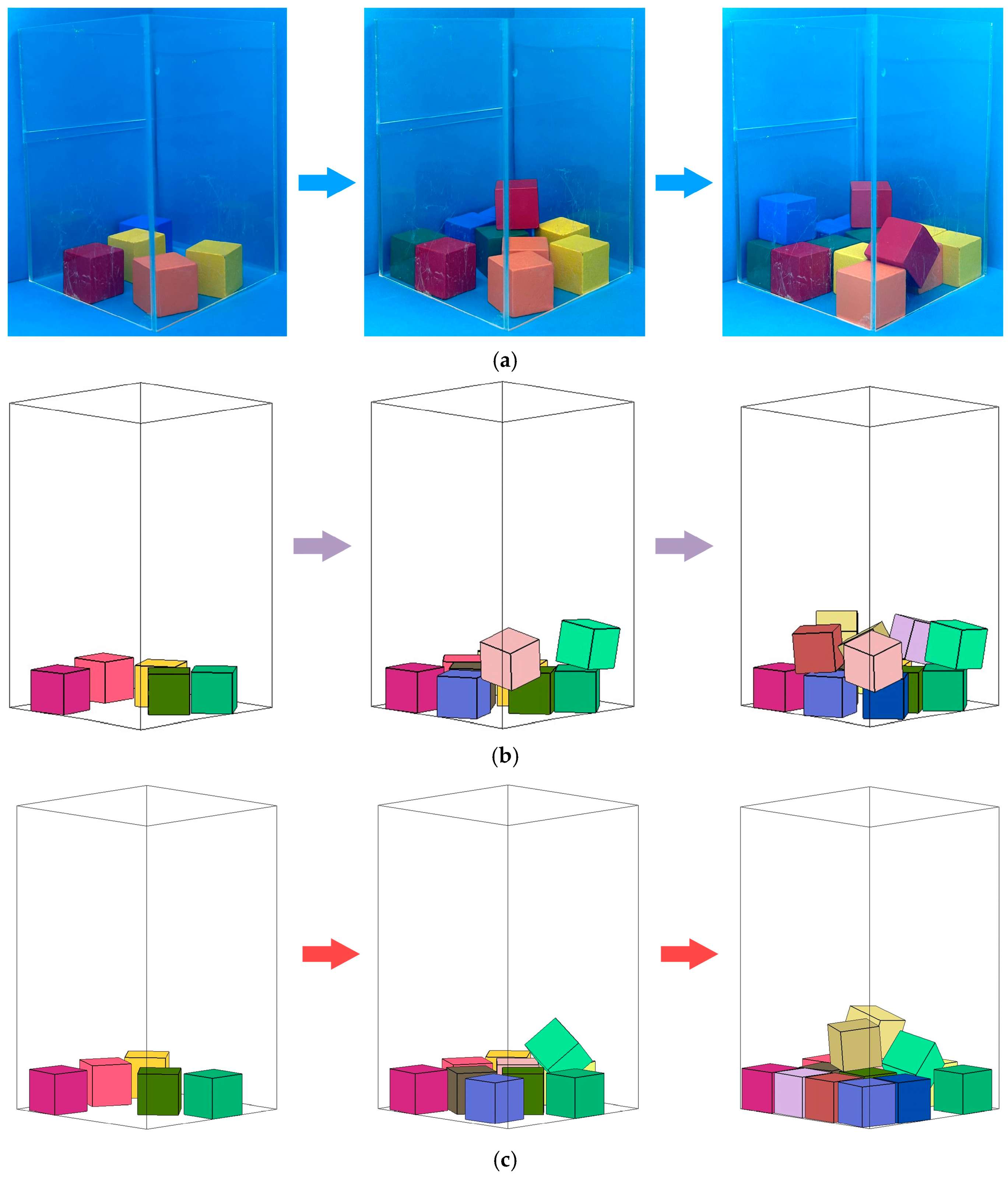
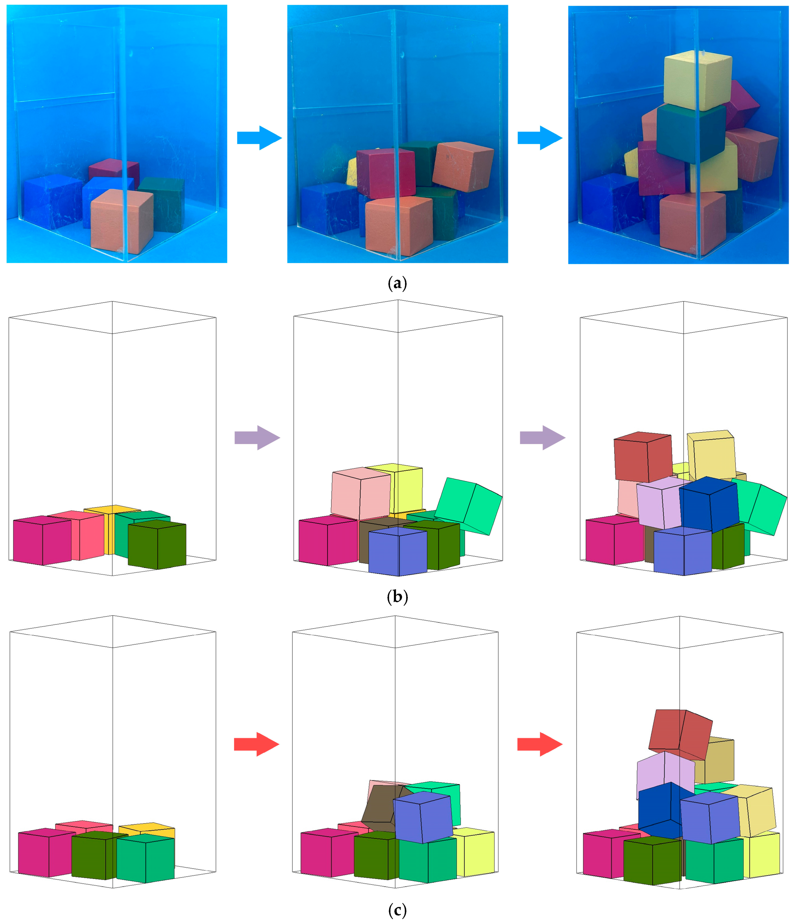
5.1. Packing Experiment of Multiple Cubes

By conducting packing experiments with granular materials, comparing the resulting packing height and packing state from the experiments with DEM simulations is an intuitive and applicable approach to validating the effectiveness and accuracy of the simulation [21,31]. In this work, three sizes of cubes with edge lengths of 20 mm, 25 mm, and 30 mm, made of Robinia wood, were selected for packing experiments. The appearance of the cubes used in the experiment is shown in Figure 15. The container used in the experiment was made from acrylic plates, which were transparent for the purposes of observing the packing situation of the cubes. The cross-sectional size of the container was 90 mm × 90 mm, and the height was 150 mm.

Three sizes of cubes were used in the packing experiment, with 15 blocks in each group. During the experiment, the container was first fixed, and a cardboard sheet with a hole in it was placed above the opening of the container to control the position and angle of each cube during the falling process. The time interval between the dropping of each cube was about 1 s, and the dropping process was continuous. The packing process was recorded using a camera during the experiment.

5.2. Comparison between Packing Experiment and Simulation

The three groups of experiments were simulated using the DEM simulation code developed in this paper. The comparison between the simulation and the experimental results is shown below.

5.2.1. Cubes with an Edge Length of 20 mm

Figure 16 shows the packing process of 15 cubes with an edge length of 20 mm, including the packing state when 5 cubes, 10 cubes, and 15 cubes were added during the experiment, as well as the corresponding packing simulation. It can be seen from the figure that the packing state obtained from the experiment and simulation is similar. The final packing height obtained from the experiment is 40 mm, and the final packing height obtained from the simulation before the improvement is 47.13 mm, resulting in a relative error of 17.86%, while the result obtained from the simulation after the improvement is 45.96 mm, with a smaller relative error of 14.9%.

5.2.2. Cubes with an Edge Length of 25 mm

Figure 17 shows the packing process of 15 cubes with an edge length of 25 mm; it can be seen that the packing state obtained from the experiment is roughly consistent with that from the simulation. The final packing height obtained from the experiment is 101 mm, while those obtained from the two DEM simulations are 87.03 mm and 103.68 mm, respectively. The relative errors between the simulation and experiment are 13.83% and 2.65%, indicating that the simulation after the improvement is more similar to the experimental result.

5.2.3. Cubes with an Edge Length of 30 mm

Figure 18 shows the packing process of 15 cubes with a side length of 30 mm. Similar to the previous two groups, the DEM code accurately simulated the experimental results of this group. The final packing height obtained from the experiment is 123 mm, while those obtained from the two simulations are 143.07 and 129.42 mm, respectively.

From the comparison of the three sets of experiments with numerical simulations, there is a closer alignment between the DEM after the improvement and the experimental results, both in terms of packing and packing height, compared to the original method. This suggests that the improved contact force model leads to an optimization of the simulation.

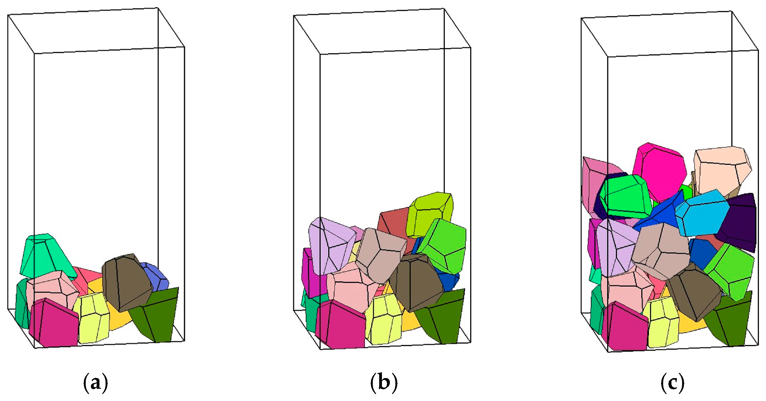
5.3. Packing Simulation of Randomly Shaped Polyhedral Elements

In reality, the shape of particles in granular systems is usually irregular. Therefore, the DEM after the improvement was extended to generate randomly shaped polyhedral elements and simulate the packing process. In the simulation, a container size of 40 cm × 40 cm × 80 cm was used, and the average particle size of the generated randomly shaped elements was 15 cm. Packing simulations were performed for 10, 20, and 30 randomly shaped elements, as shown in Figure 19. It can be observed from the figure that the packing of elements with arbitrary shapes was achieved with the simulation. Therefore, the applicability of the improved contact force model for calculating the contact force between polyhedral elements and the reliability of the DEM simulation program are further validated.

6. Conclusions

By combining the experimental and numerical simulation approaches, this study explores the contact force between polyhedral elements under various contact modes, and the following main conclusions were drawn:

• The experimental method designed in this study can be employed to test the contact forces between polyhedral blocks under different modes. A contact stiffness correction coefficient was introduced into the Cundall model, leading to the construction of an improved contact force model suitable for polyhedral elements.
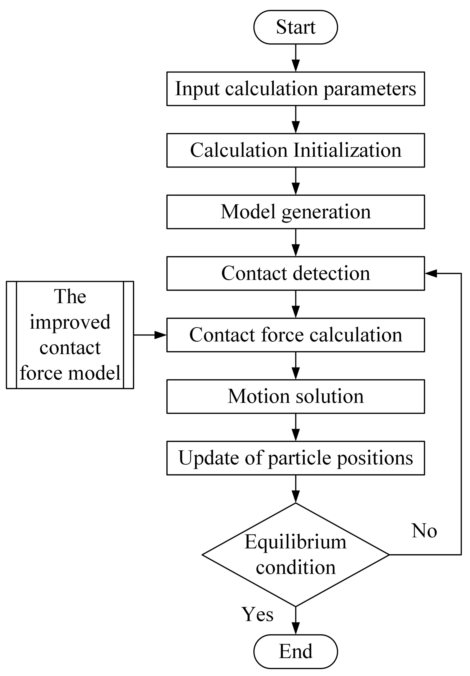
• The improved contact force model was incorporated into the DEM. An analysis of simulated contact force peaks and force patterns revealed an improved accuracy of the model, and this would affect the motion behavior of polyhedral elements.
• The DEM simulation methods, both before and after the improvement, were applied to packing experiments with cubic specimens. A comparative analysis of the results confirmed the improved accuracy and reliability of the improved contact force model in simulating the contact of polyhedral elements.

This work presents an exploration into the study of contact forces involving polyhedral elements. The proposed improved contact force model optimizes the DEM simulation of polyhedral elements, and future research could further improve experimental techniques based on this study. Additionally, there is potential to develop contact models for more complexly shaped elements for engineering applications in subsequent studies.

References

1. Horabik, J.; Molenda, M. Parameters and contact models for DEM simulations of agricultural granular materials: A review. Biosyst. Eng. 2016, 147, 206–225. [Google Scholar] [CrossRef]
2. Petalas, A.L.; Dafalias, Y.F.; Papadimitriou, A.G. SANISAND-F: Sand constitutive model with evolving fabric anisotropy. Int. J. Solids Struct. 2020, 188, 12–31. [Google Scholar] [CrossRef]
3. Das, S.K.; Das, A. Influence of quasi-static loading rates on crushable granular materials: A DEM analysis. Powder Technol. 2019, 344, 393–403. [Google Scholar] [CrossRef]
4. Liu, Y.; Wang, Y.T.; Li, X.Z. Analysis of particle crushing in rolling compaction for rockfill dam using DEM. Appl. Mech. Mater. 2013, 353, 702–705. [Google Scholar] [CrossRef]
5. Toe, D.; Bourrier, F.; Dorren, L.; Berger, F. A novel DEM approach to simulate block propagation on forested slopes. Rock Mech. Rock Eng. 2018, 51, 811–825. [Google Scholar] [CrossRef]
6. Gong, H.; Song, W.; Huang, B.; Shu, X.; Han, B.; Wu, H.; Zou, J. Direct shear properties of railway ballast mixed with tire derived aggregates: Experimental and numerical investigations. Constr. Build. Mater. 2019, 200, 465–473. [Google Scholar] [CrossRef]
7. Cil, M.B.; Alshibli, K.A. 3D analysis of kinematic behavior of granular materials in triaxial testing using DEM with flexible membrane boundary. Acta Geotech. 2014, 9, 287–298. [Google Scholar] [CrossRef]
8. Liu, G.; Li, J. A three-dimensional discontinuous deformation analysis method for investigating the effect of slope geometrical characteristics on rockfall behaviors. Int. J. Comp. Meth. 2019, 16, 455–471. [Google Scholar] [CrossRef]
9. Chen, G.; Zheng, L.; Zhang, Y.; Wu, J. Numerical simulation in rockfall analysis: A close comparison of 2-D and 3-D DDA. Rock Mech. Rock Eng. 2013, 46, 527–541. [Google Scholar] [CrossRef]
10. Munjiza, A.A. The Combined Finite-Discrete Element Method; John Wiley Sons: London, UK, 2004. [Google Scholar]
11. Mahabadi, O.K.; Randall, N.X.; Zong, Z.; Grasselli, G. A novel approach for micro-scale characterization and modeling of geomaterials incorporating actual material heterogeneity. Geophys. Res. Lett. 2012, 39, 1303. [Google Scholar] [CrossRef]
12. Kang, G.; Ning, Y.; Liu, R. Simulation of force chains and particle breakage of granular material by numerical manifold method. Powder Technol. 2021, 390, 464–472. [Google Scholar] [CrossRef]
13. Seyedan, S.; Sołowski, W.T. From solid to disconnected state and back: Continuum modelling of granular flows using material point method. Comput. Struct. 2021, 251, 106545. [Google Scholar] [CrossRef]
14. Liu, C.; Sun, Q.; Zhou, G.G.D. Coupling of material point method and discrete element method for granular flows impacting simulations. Int. J. Numer. Meth. Eng. 2018, 115, 172–188. [Google Scholar] [CrossRef]
15. Cundall, P.A. A computer model for simulating progressive, large-scale movement in blocky rock system. In Proceedings of the International Symposium on Rock Mechanics, Nancy, France, 4–6 October 1971; pp. 129–136. [Google Scholar]
16. Huang, Y.; Sun, W.; Xie, Q.; You, H.; Wu, K. Discrete Element Simulation of the Shear Behavior of Binary Mixtures Composed of Spherical and Cubic Particles. Appl. Sci. 2023, 13, 9163. [Google Scholar] [CrossRef]
17. Nassauer, B.; Kuna, M. Contact forces of polyhedral particles in discrete element method. Granul. Matter. 2013, 15, 349–355. [Google Scholar] [CrossRef]
18. Orozco, L.F.; Delenne, J.Y.; Sornay, P.; Radjai, F. Discrete-element model for dynamic fracture of a single particle. Int. J. Solids Struct. 2019, 166, 47–56. [Google Scholar] [CrossRef]
19. Kildashti, K.; Dong, K.; Yu, A. Contact force models for non-spherical particles with different surface properties: A review. Powder Technol. 2023, 418, 118323. [Google Scholar] [CrossRef]
20. Cundall, P.A. Formulation of a three-dimensional distinct element model—Part I. A scheme to detect and represent contacts in a system composed of many polyhedral blocks. A scheme to detect and represent contacts in a system composed of many polyhedral blocks. Int. J. Rock Mech. Min. 1988, 25, 107–116. [Google Scholar] [CrossRef]
21. Liu, G.; Xu, W.; Zhou, Q. DEM contact model for spherical and polyhedral particles based on energy conservation. Comput. Geotech. 2023, 153, 105072. [Google Scholar] [CrossRef]
22. Feng, Y.T.; Owen, D.R.J. A 2D polygon/polygon contact model: Algorithmic aspects. Eng. Comput. 2004, 21, 265–277. [Google Scholar] [CrossRef]
23. Feng, Y.T.; Han, K.; Owen, D.R.J. Energy-conserving contact interaction models for arbitrarily shaped discrete elements. Comput. Method. Appl. Mech. 2012, 205, 169–177. [Google Scholar] [CrossRef]
24. Rojek, J.; Karlis, G.F.; Malinowski, L.J.; Beer, J. Setting up virgin stress conditions in discrete element models. Comput. Geotech. 2013, 48, 228–248. [Google Scholar] [CrossRef] [PubMed]
25. Minamoto, H.; Kawamura, S. Effects of material strain rate sensitivity in low speed impact between two identical spheres. Int. J. Impact Eng. 2009, 36, 680–686. [Google Scholar] [CrossRef]
26. Cole, D.M.; Mathisen, L.U.; Hopkins, M.A.; Knapp, B.R. Normal and sliding contact experiments on gneiss. Granul. Matter 2010, 12, 69–86. [Google Scholar] [CrossRef]
27. Ouyang, Y.; Yang, Q.; Chen, X. Bonded-particle model with nonlinear elastic tensile stiffness for rock-like materials. Appl. Sci. 2017, 7, 686. [Google Scholar] [CrossRef]
28. Liu, P.; Liu, J.; Gao, S.; Wang, Y.; Zheng, H.; Zhen, M.; Zhao, F.; Liu, Z.; Ou, C.; Zhuang, R. Calibration of Sliding Friction Coefficient in DEM between Different Particles by Experiment. Appl. Sci. 2023, 13, 11883. [Google Scholar] [CrossRef]
29. Nadler, B.; Guillard, F.; Einav, I. Kinematic model of transient shape-induced anisotropy in dense granular flow. Phys. Rev. Lett. 2018, 120, 198003. [Google Scholar] [CrossRef]
30. Malone, K.F.; Xu, B.H. Determination of contact parameters for discrete element method simulations of granular systems. Particuology 2008, 6, 521–528. [Google Scholar] [CrossRef]
31. Mack, S.; Langston, P.; Webb, C.; York, T. Experimental validation of polyhedral discrete element model. Powder Technol. 2011, 214, 431–442. [Google Scholar] [CrossRef]
Figure 1. Design of specimens: (a) specimen with a thickness of 6 cm; (b) specimen with a thickness of 2 cm.
Applsci 14 00311 g001
Figure 2. Force hammer loading device.
Applsci 14 00311 g002
Figure 3. Connection of experimental equipment.
Applsci 14 00311 g003
Figure 4. Different contact modes of specimens: (a) edge–edge-collinear; (b) edge–point; (c) point–face; (d) edge–edge-noncollinear; (e) edge–face; (f) face–face.
Applsci 14 00311 g004aApplsci 14 00311 g004b
Figure 5. Arrangements of strain gauges for different contact modes: (a) edge–edge; (b) edge–point; (c) point–face; (d) edge–edge/edge–face; (e) face–face.
Applsci 14 00311 g005
Figure 6. Schematic diagram of strain calculation for edge–face contact mode.
Applsci 14 00311 g006
Figure 7. The modified fitting curve of dimensionless contact force under different contact modes.
Applsci 14 00311 g007
Figure 8. The calculation process of DEM simulation program.
Applsci 14 00311 g008
Figure 9. Comparison of DEM and experimental contact force–time curves under edge-to-edge contact mode (collinear).
Applsci 14 00311 g009
Figure 10. Comparison of DEM and experimental contact force–time curves under edge-to-edge contact mode (non-collinear).
Applsci 14 00311 g010
Figure 11. Comparison of DEM and experimental contact force–time curves under point-to–edge contact mode.
Applsci 14 00311 g011
Figure 12. Comparison of DEM and experimental contact force–time curves under point-to-face contact mode.
Applsci 14 00311 g012
Figure 13. Comparison of DEM and experimental contact force–time curves under edge-to-face contact mode.
Applsci 14 00311 g013
Figure 14. Comparison of DEM and experimental contact force–time curves under face-to–face contact mode.
Applsci 14 00311 g014
Figure 15. The cubes and container used in the packing experiment: (a) cubic specimens; (b) transparent container.
Applsci 14 00311 g015
Figure 16. The packing process of 15 cubes with an edge length of 20 mm: (a) experiment; (b) DEM before the improvement; (c) DEM after the improvement.
Applsci 14 00311 g016
Figure 17. The packing process of 15 cubes with an edge length of 25 mm: (a) experiment; (b) DEM before the improvement; (c) DEM after the improvement.
Applsci 14 00311 g017
Figure 18. The packing process of 15 cubes with an edge length of 30 mm: (a) experiment; (b) DEM before the improvement; (c) DEM after the improvement.
Applsci 14 00311 g018
Figure 19. Packing simulation of randomly shaped elements: (a) 10 cubes; (b) 20 cubes; (c) 30 cubes.
Applsci 14 00311 g019