Intelligent Space Object Detection Driven by Data from Space Objects

Abstract

With the rapid development of space programs in various countries, the number of satellites in space is rising continuously, which makes the space environment increasingly complex. In this context, it is essential to improve space object identification technology. Herein, it is proposed to perform intelligent detection of space objects by means of deep learning. To be specific, 49 authentic 3D satellite models with 16 scenarios involved are applied to generate a dataset comprising 17,942 images, including over 500 actual satellite Palatino images. Then, the five components are labeled for each satellite. Additionally, a substantial amount of annotated data is collected through semi-automatic labeling, which reduces the labor cost significantly. Finally, a total of 39,000 labels are obtained. On this dataset, RepPoint is employed to replace the 3 × 3 convolution of the ElAN backbone in YOLOv7, which leads to YOLOv7-R. According to the experimental results, the accuracy reaches 0.983 at a maximum. Compared to other algorithms, the precision of the proposed method is at least 1.9% higher. This provides an effective solution to intelligent recognition for spatial target components.

1. Introduction

With the constant progress in space exploration, there has been a significant advancement of such technologies as positioning and navigation, satellite communication, remote observation, surveillance, and reconnaissance, all of which rely on the use of satellites. At present, they play an increasingly important role in both civil engineering and national defense. However, the accumulation of space debris and retired satellites poses a severe threat to operational satellites. Therefore, it is imperative to minimize the safety risk of in-orbit satellites by enabling satellites to automatically identify the targets in the surrounding environment [1]. In recent years, various image sensors have been widely applied on satellites to enhance their capability to perform detection in the surrounding environment, which is significant to the development of image-based space object detection methods [2,3].

In 2014, Richard Linares proposed that shape estimation can be treated as the most likely shape model, with each filter operating based on unscented estimation. Thus, the time brightness of resident space objects is combined with angular data to leverage fusion sensitivity, thus creating the models and associated trajectories of resident space objects. In 2016, Timothy S. Murphy used matched filters and Bayesian methods to detect the target in space. Subsequently, Richard Linares tracked and characterized both active and inactive space objects for the description and classification of features of space debris. In 2017, Xueyang Zhang proposed to detect the objects through the correlation between the motion of objects over multiple frames and the attitude-related information about satellites. By using the video footage captured by the Tian Tuo-2 satellite, the algorithm showed a massive potential in space target detection. In 2018, Yan Z pioneered applying CNNs to spacecraft detection. Then, an improved regression-based convolutional neural network named YOLOv2 was adopted to detect the spacecraft in the images. In 2019, Xi Yang introduced a new method based on multi-model adaptive estimation to determine the most likely shape of resident space objects through multiple candidate shape models. Meanwhile, the observed inertial orientation and trajectory of resident space objects were recovered. This method proved effective in identifying the model and state of residential objects in space. Proposed by Tan Wu, a space target recognition network (T-SCNN) was shown to achieve a high accuracy in recognition. In 2020, Xi Yang put forward a mixed R-CNN with partial semantic information for space target recognition, with the main components of detected satellites segmented. In 2021, the University of Luxembourg introduced the SPARK space satellite dataset as a novel and unique multimodal image dataset of space objects to classify spacecraft and debris into 11 categories in total. In 2022, Song J presented the Spacecraft Pose Network (SPN), in which the regions within 2D bounding boxes were used to determine the relative pose. Then, regression was performed to obtain finer estimates. Through the SPN method, the relative positions were estimated by leveraging the constraints imposed by the detected 2D bounding boxes and the estimated relative poses [4,5,6,7,8,9,10,11,12,13].

With the accumulation of data and the continuous development of artificial intelligence technology, deep learning has been widely practiced to improve the performance in object detection. In terms of generalized object detection, Alex Krizhevsky et al. pioneered proposing the deep convolutional neural network [14]. Subsequently, other researchers like Alex Krizhevsky integrated deep neural networks with image object detection to yield a series of effective works, progressing from R-CNN to Fast R-CNN, and further to Faster R-CNN [15,16,17]. These works laid a foundation for the development of classical architectures intended for object detection. However, the limitations of the R-CNN architecture make detection a time-consuming process in certain scenarios. To address this problem, Redmon et al. introduced a regression-based object detection algorithm called YOLO (You Only Look Once) [18]. It significantly improved the speed of detection while maintaining a certain level of accuracy. Liu et al. integrated the regression of YOLO with the anchor box mechanism of Faster R-CNN, through which the SSD (Single Shot MultiBox Detector) algorithm was developed [19]. This algorithm maintained the high performance of YOLO in time efficiency while ensuring the satisfactory outcome of precise bounding box localization. Redmon et al. continued improving the YOLO algorithm, which promoted the development of YOLO9000 [20], YOLOv3, and subsequently YOLOv7 frameworks [20,21,22,23].

Due to the high cost and difficulty in collecting space data, most space target datasets are generated through model simulation [24]. Also, the complexity of real imaging in space is ignored. In space, the targets are set against a cluttered background, with variations in altitude. Meanwhile, they are subject to the impact of various cosmic rays, solar storms, and thermal noise from electronic devices, among others [25]. In light of this, it is proposed in this study to simulate real space scenes through multi-image fusion [26]. To be specific, 49 real satellite 3D models, involving 500 real satellite images, were applied to create an original dataset of 17,942 images. Through semi-automatic labeling, five components of the satellite were annotated to obtain a total of 39,000 labels, making it one of the few large-scale datasets for space target component recognition. Furthermore, RepPoint was used to optimize the ELAN module of YOLOv7, which led to the ELAN-R module. Also, the YOLOv7-R model was proposed. This algorithm model, as verified on the dataset, outperforms other existing algorithm models in accuracy by at least 1.9%.

The main contributions of this paper are summarized as follows:

• A space target component detection dataset of 17,942 images was created;
• An image fusion method was adopted to simulate the real scenarios in space to the maximum extent;
• Semi-automatic labeling was performed for dataset annotation, which reduced the cost of manual annotation significantly;
• The YOLOv7-R model algorithm was proposed, whose better performance was verified.

2. Dataset Construction and Labeling

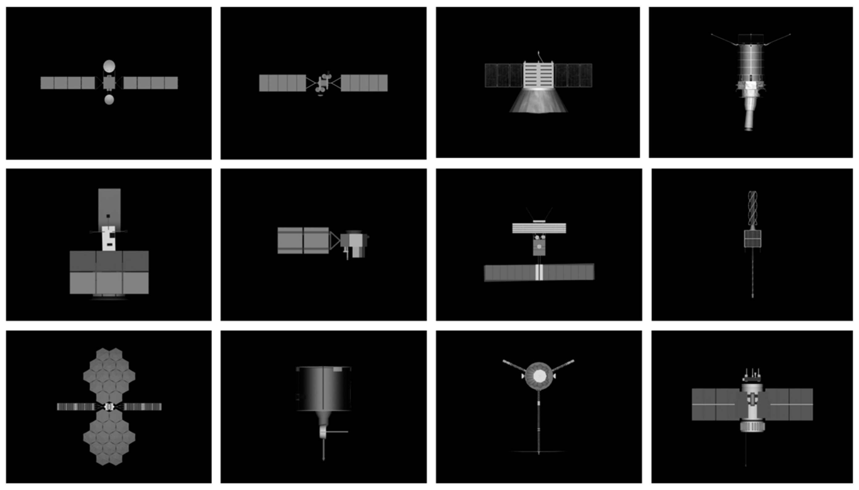
2.1. Dataset Construction

It is challenging to collect such data due to the limitations of observation conditions and external environments. However, the load structure and characteristics of various space objects are known to the observer. Through computer simulation, it is possible to generate a large number of synthetic images with labeled information under some particular observational conditions. When these synthetic images are combined with a small proportion of real data, transfer learning is performed to detect space objects [27].

In the present study, 49 3D satellite models are applied to create a dataset with a comprehensive orientation. The initial dataset consists of over 9600 images, including 2300 images from the BUAA-SID 1.0 dataset. It was constructed by Beihang University in response to the needs of a specific project, whose contents have not been fully disclosed. The meaning of BUAA-SID is not discernable from the available information. In the original paper, it is referred to as the Satellite Image Dataset (640 × 480 resolution). It includes 20 satellite models [28], 6200 images (640 × 480 resolution) with 29 satellite models, and 500 actual satellite images. An additional 500 images were collected online. Due to the discrepancy in image size between the satellite dataset and the dataset collected online, they were uniformly resized to 600 × 600. Finally, a large-scale satellite dataset with two different sizes was created. Based on space object 3D models, the BUAA-SID 1.0 space object image database uses 3ds Max 2009 software to produce the sequence of a full-viewpoint simulation image. It involves 56 3D satellite models and their simulation images. The BUAA-SID 1.0 simulated image database consists of 25,760 simulated images whose resolution is 320 × 240 pixels, with 460 images in each satellite. Among them, 230 images are full-view 24-bit color images, and the other 230 images are the corresponding binary images. With 20 full-view 24-bit color satellite simulation images selected from the BUAA-SID 1.0 dataset, 115 images of various postures are chosen for each satellite. Through bilinear interpolation, the resolution of these images increased to 640 × 480 pixels. Figure 1 shows some of the satellite images.

In this paper, the process of generating a space object image by simulation is detailed as follows:

Due to the limited amount of data available in the BUSSA-SID1.0 dataset, it is difficult to perform deep learning on large datasets. Therefore, the construction of the BUAA-SID1.0 dataset is simulated and the software Blender3.4 is applied to model 29 different types of space objects. In order to reflect the dynamic characteristics of these space objects faithfully, their motion is simulated by rotating and moving these models in the Blender software. In the 3D model library, the strong rendering capability of Blender is exercised to conduct imaging simulation of 3D models, as shown in Figure 2.

The critical steps in the generation of images within the simulation image library are detailed as follows:

• Camera Setup: In space-based visible light imaging detection of space targets, there is a long distance between the space target and the camera, and the distance of observation far exceeds the size of the space observation target. Therefore, orthographic projection is performed in the process of simulation. Also, a camera is used for alignment with the satellite, with a field of view set to 45°. Thus, both are aligned with the z-axis. This allows the model to be positioned at the center of the camera in the initial state, which makes all parts visible.
• Light Source Setup: In the space environment, sunlight is almost comparable to parallel light. Hence, a parallel white light source is introduced at the initial position of the camera. Without attenuation, it has an intensity multiplier coefficient of 0.906. By adjusting this multiplier coefficient, it is achievable to obtain the simulated images with varied brightness.
• Adjusting Positions: There are different viewpoints and lighting conditions because of the changes in the relative positions between the camera, light source, and satellite model. To capture the simulated images from all viewpoints, the position of light source relative to the camera is kept unchanged and the model remains stationary, while the camera is moved along the Earth’s spherical surface centered on the satellite model. By means of latitude and longitude representation as a geographic method, sampling is conducted along the 0° to ±90° latitude line, which leads to 210 sampling viewpoints.
• Model Rendering Output: The output image resolution is set to 640 × 480 pixels, and the image attribute is set to 256-bit pixels, with the contour information of the target retained effectively.

After being rendered through 3D modeling software Blender3.4., these images are converted into a total of 6200 high-resolution spatial object images. Some of these images are shown in Figure 3.

In addition, Figure 4 presents a small amount of real data obtained in this paper, as authorized for use by the original authors, and the simulation dataset collected by the authors of this paper from the website.

2.2. Data Enhancement

In this study, 8282 simulated images captured by 49 satellites are used for scene simulation. Firstly, the color images are converted into grayscale images, and Gaussian filtering is performed to remove noise from the images [29]. Secondly, the Sobel operator is employed to calculate the gradient magnitude and direction of the images [30], while non-maximum suppression is performed to eliminate non-edge points and refine the edges. The upper and lower threshold values of binarization are set to 30 and 150, respectively, which removes redundant pixels from the images, with a sharpened edge image obtained. Then, the binary image is combined with the original image at a 0.2:0.8 ratio to capture a feature image with distinct edge characteristics. There are sixteen background images selected, including the color images of the Earth and deep space backgrounds, as well as the grayscale images of the Earth and deep space backgrounds. To evenly distribute the backgrounds of the satellites and better perform the simulation, the dataset is randomly divided into 16 groups comprising about 500 images each. Each group is fused with the background image of the same type [31]. During the fusion process, an appropriate proportion of the background, ranging from 0.17 to 0.25, is chosen. Gaussian noise is also added to this part to simulate the sources of various natural and artificial noises, such as the thermal noise made by electronic devices and the celestial noise made in astronomical observations. The reason why Gaussian noise is chosen lies in the Gaussian distribution, followed by the random noise introduced by various factors in the process of image acquisition, transmission, and processing which follows [32]. After multiple experimental comparisons performed to minimize image distortion, the Gaussian noise with a mean of 0 and a variance of 0.001 is added into this part of the dataset. The process of image fusion is illustrated in Figure 5, and the final results are presented in Figure 6.

2.3. Dataset Labeling

Dataset labeling plays a crucial role in the construction of a dataset, which has a significant impact on the final outcome of training. Typically, dataset labeling is carried out manually by using various open-source labeling tools like labelimg. As for image object detection, it requires the areas of interest in the images to be manually marked, including the coordinates, sizes, and categories of the objects. However, this process is labor-intensive, time-consuming, and often inefficient. In this study, there is a specific challenge encountered in satellite object detection, requiring the use of a large-scale dataset with different classes and object poses. Unfortunately, the available satellite images are not labeled, which necessitates manual labeling efforts. To reduce the workload, semi-automatic labeling is performed. To begin with, a lightweight model is trained on a subset of already labeled data, which facilitates the automatic labeling of the remaining unlabeled data [33]. Subsequently, the automatically generated labels are manually corrected to rectify any mislabeling or omissions. Through this approach, both labor and time costs are significantly reduced. Meanwhile, the large-scale acquisition of high-quality labeled data is promoted, which is essential for the development of an effective satellite object detection model.

In this paper, a total of 1000 images are manually labeled. There are five categories of label for each image: “Panel”, “Body”, “Antenna”, “Optical-load”, and “Antenna-rod”, as shown in

Table 1. Satellite components and abbreviations reference table.

Solar Panels on Satellites	Body of the Satellite	Circular Antenna on Satellites	Optical Payload on Satellites	Antenna Array on Satellites
panel	body	antenna	optical-load	antenna-rod

. To improve the effectiveness of semi-automatic labeling, dozens of images are randomly labeled for each category of satellites, which improves dataset distribution for the image categories to be balanced.

Considering the similarities in appearance between airplanes and satellites, the parameters learned by the model on a remote sensing airplane dataset are effectively transferred for the training on a satellite dataset. Moreover, due to the scarcity of manually annotated datasets, transfer learning is conducive to accelerating the convergence of training satellite models. Thus, the performance in training is improved for smaller models. Named “plane”, the model trained on the remote sensing airplane dataset using YOLOv5s reaches 0.99 in precision. This method of semi-automatic labeling relies on a pre-trained remote sensing aircraft model (plane) constructed through transfer learning [34]. It undergoes 300 iterations with a batch size of 86, resulting in a small model with a training accuracy of 0.852. Then, this model is used to predict the labels for 6300 unlabeled data points. Since the model is unfit for completely correct prediction, manual screening is performed to remove the incorrectly labeled data. Additionally, human–computer interaction is performed to obtain accurately labeled high-quality datasets. In combination with the labeled datasets, they comprise a larger dataset for subsequent training. Semi-automatic labeling is suitable to transform the role of annotators from data labeling to data verification, thus enhancing work efficiency significantly.

According to the experimental results, the lightweight model constructed by using plane as the model pre-trained on fewer samples performs better in detection [35]. The ultimate accuracy of labeling is consistently above 94%, with the best performance achieved on the label of “panel” given an accuracy of 0.98. The label of “body”, which is more complex in shape but with no consistency in pattern, maintains an accuracy of 0.95 or higher. In comparison, the labels like “antenna”, “optical-load”, and “antenna-rod” perform slightly worse when the accuracy is maintained at above 0.9, despite those missing and incorrect labels. After an analysis of this issue, this is found to result mainly from a significant variation between these three label categories within the dataset. To compound this, they are characterized by a confined area and low quantity, which hampers the capability to train a robust labeling model for these categories given a small sample size. It is also implied that semi-automatic labeling is unlikely to completely replace manual labeling. Overall, this interactive, task-specific method of semi-automatic labeling demonstrates a significant advantage over manual labeling in time cost and the complexity of labeling, as evidenced by the final results of labeling shown in Figure 7.

3. Space Object Detection Algorithm Model

3.1. Introduction to YOLOv7

As one of the most advanced single-stage object detection algorithms, the YOLO series of algorithms is applied to perform various computer vision tasks. YOLOv7, a recent iteration, introduces two new efficient network architectures, namely ELAN (Efficient layer aggregation networks) and E-ELAN (Extended efficient layer aggregation networks), with model reparameterization incorporated into the network architecture. Given the same model size, YOLOv7 outperforms YOLOv3, YOLOv5, and YOLOX in terms of accuracy and speed. The architecture diagram of YOLOv7’s feature extraction network [36] shown in Figure 8b.

In this paper, YOLOv7-R is built upon YOLOv7, with a convolution module introduced into ELAN to obtain the ELAN-R module. As a result, the accuracy is improved significantly. Combining CSP (Ross Stage Partial) and SPP (Spatial Pyramid Pooling) structures, the spatial pyramid pooling with the context-sensitive context (SPPCSPC) module is retained, as shown in Figure 8d. Through the CSP structure, the input features are divided into two branches, of which one is for feature extraction through convolution layers and the other is for SPP processing. This structure reduces computational workload while accelerating processing. In the SPP structure, four different max-pooling operations are conducted to generate various receptive fields, making the algorithm adaptable to different image resolutions. In the final detection layer, the network is used to predict the objects of different sizes on the corresponding feature maps and non-maximum suppression is performed to remove the highly redundant prediction boxes, which leads to the final prediction results.

3.2. ELAN

A typical network design focuses on parameters, computation, and computational density. The ELAN module adopts the following design strategies to build an efficient network, applying control on the length of the longest and shortest gradient paths for effective learning and convergence in deeper networks, as shown in Figure 8a. In large-scale ELAN, a stable state can be reached, regardless of the length of gradient path and the number of stacked computation blocks. The ELAN module consists of two branches. Among them, one changes channel numbers through a 1 × 1 convolution, while the other adjusts channel numbers through a 1 × 1 convolution and then performs feature extraction with four 3 × 3 convolutions to merge the four features for the final results of feature extraction. ELAN relies on group convolution to increase the cardinality of features, combining the features of different groups through shuffle and merge operations without any change in the paths of gradient propagation in the original architecture. This operation enhances the features learned by different feature maps, thus improving the utilization of parameters and computations.

3.3. RepPoints and ELAN-R

As shown in Figure 9, RepPoint is a set of points that learns to position itself above the object flexibly, which restricts the spatial range of the object, representing the locally significant regions with important semantic information [37,38,39]. The training of RepPoint is jointly driven by object localization and detection, making it closely related to the ground-truth bounding boxes. Also, the detector is guided to correctly classify the objects. The bounding box is a four-dimensional representation purposed to encode the spatial position of the object, i.e., $B=(x, y, w, h)$, where x and y represent the center point, while w and h represent the width and height, respectively. Modern object detectors rely on bounding boxes to represent the objects at various stages of the detection process. However, the four-dimensional bounding box allows the position of an object to be roughly represented, considering only the rectangular spatial extent of the object. However, this overlooks the information about the shape of the object, its pose, and the position of semantically important local areas, which enhances the accuracy of localization and improves the outcome of object feature extraction [40]. To overcome these limitations, RepPoints introduces a set of adaptive sample points for modeling [41], which is expressed as follows:

$$\mathcal{R}=\left\{\right(x_k,y_k){\}}_{k=1}^n$$

(1)

where n represents the total number of sample points used for representation. The default value of n is set to 9. The learning of RepPoint is driven by both object localization loss and object detection loss. To calculate object localization loss, a transformation function τ is first applied to convert RepPoints into pseudo-boxes. Then, the difference between the transformed pseudo-boxes and the ground-truth bounding boxes is computed as follows.

$${R_r=\left\{\right(x_k+\Delta x_k,y_k+\Delta y_k\left)\right\}}_{k=1}^n$$

(2)

where ${\{\Delta x_k,\Delta y_k\}}_{k=1}^n$ represents the offsets. Unlike the inconsistency of scale in traditional bounding box regression parameters, all the offsets in the process of refining RepPoint are dealt with on the same scale. Thus, scale discrepancy is prevented. During training, annotation is required in the form of bounding boxes, and prediction is converted into the bounding box during evaluation. This requires the transformation of RepPoint into a bounding box. A predefined transformation function τ is used to achieve this purpose: Rp-Bp, where Rp represents the RepPoint of an object P, and τ(Rp) represents the pseudo-box. The transformation function T is used to perform a minimum-maximum operation along the two axes to determine Bp as follows.

$$T=\{(ma{x}_{{}_x}^i(R_r),mi{n}_x^j(R_r)),(ma{x}_y^k(R_r),mi{n}_y^l(R_r))\}$$

(3)

where i, j, k, and l represent the maximum and minimum points along the x-axis and the maximum and minimum points along the y-axis on $R_r$, respectively, which is the bounding box over the sample points. By replacing the 3 × 3 convolution kernel in the backbone with RepPoint, ELAN-R is obtained. In the core part, the original ELAN modules are still used. With these modifications, YOLOv7-R is created to enhance the capability of the model in terms of geometric deformation modeling [42], as shown in Figure 8a.

4. Experimental Results and Analysis

The experiment conducted in this study involves a dataset comprising 17,942 images, including 500 real data images. The size of the input image is 640 × 640. For random allocation, the training-test split ratio is set to 8:2. The experiment was conducted on Ubuntu 18.04, using two NVIDIA A5000 GPUs (NVIDIA Corporation, Santa Clara, CA, USA), each of which has a VRAM of 24 GB, an AMD 7371 CPU (Advanced Micro Devices, Inc. Santa Clara, CA, USA), and a RAM of 56 GB. A pre-trained remote sensing plane model was taken as the initial model. During training, each batch size was set to 30, and training was performed for 300 epochs. Initially set to 0.01, the learning rate was gradually reduced to 0.001 under a cosine decay strategy. In the optimization algorithm, the Adam optimizer with a momentum parameter of 0.937 and a weight decay of 0.0005 was used. The loss function relied on CIoU loss [43] for object localization and on cross-entropy loss for classification. Data enhancement involved various operations such as Mosaic image stitching, image translation, scaling, distortion, flipping, and the random adjustment of hue, saturation, and brightness. Additionally, the MixUp image blending technique was applied to enhance the diversity of data.

To improve the efficiency and robustness of training, multi-scale training and rectangular box inference techniques were applied. In this way, the high accuracy of training was achieved, as shown in

Table 2. Comparison of training results between YOLOv3 through the ResNet53 network architecture, YOLOv7, and YOLOv7-R. The difference between the two lies in the backbone module, with YOLOv7 as the ELAN module and YOLOv7-R as the ELAN-R module. In other YOLO models, the network structures with a similar number of parameters are adopted.

	Panel	Body	Antenna	Optical-Load	Antenna-Rod	Accuracy
YOLOv3	0.915	0.931	0.934	0.892	0.905	0.927
YOLOv4	0.979	0.98	0.965	0.936	0.952	0.963
YOLOv5l	0.941	0.939	0.933	0.892	0.963	0.934
YOLOv6l	0.975	0.975	0.957	0.945	0.957	0.962
YOLOv8l	0.98	0.982	0.968	0.955	0.95	0.969
YOLOR	0.979	0.981	0.96	0.948	0.96	0.966
YOLOv7	0.978	0.983	0.962	0.938	0.959	0.964
YOLOv7-R	0.986	0.99	0.972	0.974	0.993	0.983

. In this experiment, the single-stage object detection models from the YOLO series were adopted, all of which were of the same parameter scale. According to the experimental results, all the models from the YOLO series achieved an accuracy of over 0.92 on the space object dataset, with 0.983 as the maximum. Concerning the accuracy achieved for each component, the “antenna-rod” performed best in YOLOv7-R, reaching 0.993. By contrast, the “optical-load” performed worst in YOLOv3, despite reaching 0.892. After the introduction of RepPoint, a significant improvement of accuracy was achieved. Compared to YOLOv7, the YOLOv7-R enhanced with RepPoint was improved by 1.9 percentage in accuracy. The detection results are presented in Figure 10, which shows the comparison in accuracy among different models. With ResNet53 as the backbone network, YOLOv3 performs worse in feature extraction compared to other advanced models, achieving an overall accuracy of 0.927. By using the ELAN module for feature extraction, YOLOv7 achieved a higher accuracy of 0.964. The ELAN module, which restricts the longest and shortest paths, enables the network to learn semantic information in more depth and accelerate convergence. Enhanced with the RepPoint module, YOLOv7-R achieved the best training results, reaching an accuracy of 0.983. This is attributed to the introduction of the RepPoint module, which improved the performance of the backbone network in extracting feature information from satellite images. RepPoint enables precise localization at the semantically meaningful positions, allowing for the refined localization. Also, the extraction of object features was improved in the process of subsequent detection. Given the fact that object detection feedback does not necessarily promote the object detection represented by bounding boxes, the advantages of RepPoint in flexible object representation are confirmed.

5. Conclusions

With the constant advancement of space exploration, there has been an increase in the demand for various relevant technologies. However, it remains challenging to obtain real satellite data. In this paper, the data obtained from 3D satellite models is not technically processed to simulate the real space satellite images as much as possible. By applying deep learning to a novel domain, satisfactory results are obtained. Nonetheless, there remain certain limitations. Most of the realistic remote sensing images are large in size, which requires the consumption of a significant amount of memory during training. The application of compression techniques might lead to the loss of features for small objects and a decrease in the accuracy of detection. Due to the scarcity of genuine satellite data, the dataset lacks diversity in terms of object variations. Thus, there is considerable room for optimizing deep learning detection models, especially in the accurate identification of ultra-small objects. To sum up, further exploration is required in these aspects.

References

1. Sharma, S.; D’Amico, S. Neural Network-Based Pose Estimation for Noncooperative Spacecraft Rendezvous. IEEE Trans. Aerosp. Electron. Syst. 2020, 56, 4638–4658. [Google Scholar] [CrossRef]
2. Phisannupawong, T.; Kamsing, P.; Torteeka, P.; Channumsin, S.; Sawangwit, U.; Hematulin, W.; Jarawan, T.; Somjit, T.; Yooyen, S.; Delahaye, D.; et al. Vision-Based Spacecraft Pose Estimation via a Deep Convolutional Neural Network for Noncooperative Docking Operations. Aerospace 2020, 7, 126. [Google Scholar] [CrossRef]
3. Hoang, D.A.; Chen, B.; Chin, T.-J. A Spacecraft Dataset for Detection, Segmentation and Parts Recognition. In Proceedings of the 2021 IEEE/CVF Conference on Computer Vision and Pattern Recognition Workshops (CVPRW), Nashville, TN, USA, 19–26 June 2021. [Google Scholar]
4. Sato, T.; Wakayama, T.; Tanaka, T.; Ikeda, K.-I.; Kimura, I. Shape of Space Debris as Estimated from Radar Cross Section Variations. J. Spacecr. Rocket. 1994, 31, 665–670. [Google Scholar] [CrossRef]
5. Rossi, A. The Earth Orbiting Space Debris. Serbian Astron. J. 2005, 170, 1–12. [Google Scholar] [CrossRef]
6. Linares, R.; Furfaro, R. Space Object classification using deep Convolutional Neural Networks. In Proceedings of the 2016 19th International Conference on Information Fusion (FUSION), Heidelberg, Germany, 5–8 July 2016. [Google Scholar]
7. Zhang, X.; Xiang, J.; Zhang, Y. Space object detection in video satellite images using motion information. Int. J. Aerosp. Eng. 2017, 2017, 1024529. [Google Scholar]
8. Yan, Z.; Song, X. Spacecraft Detection Based on Deep Convolutional Neural Network. In Proceedings of the 2018 IEEE 3rd International Conference on Signal and Image Processing (ICSIP), Shenzhen, China, 13–15 July 2018. [Google Scholar]
9. Yang, X.; Wu, T.; Zhang, L.; Yang, D.; Wang, N.; Song, B.; Gao, X. CNN with spatio-temporal information for fast suspicious object detection and recognition in THz security images. Signal Process. 2019, 160, 202–214. [Google Scholar] [CrossRef]
10. Wu, T.; Yang, X.; Song, B.; Wang, N.; Gao, X.; Kuang, L.; Nan, X.; Chen, Y.; Yang, D. T-SCNN: A Two-Stage Convolutional Neural Network for Space Target Recognition. In Proceedings of the 2019 IEEE International Geoscience and Remote Sensing Symposium, Yokohama, Japan, July 28–August 2 2019. [Google Scholar]
11. Yang, X.; Wu, T.; Wang, N.; Huang, Y.; Song, B.; Gao, X. HCNN-PSI: A hybrid CNN with partial semantic information for space target recognition. Pattern Recognit. 2020, 108, 107531. [Google Scholar] [CrossRef]
12. Musallam, M.A.; Al Ismaeil, K.; Oyedotun, O.; Perez, M.D.; Poucet, M.; Aouada, D. SPARK: Spacecraft recognition leveraging knowledge of space environment. arXiv 2021, arXiv:2104.05978. [Google Scholar]
13. Song, J.; Rondao, D.; Aouf, N. Deep learning-based spacecraft relative navigation methods: A survey. Acta Astronaut. 2022, 191, 22–40. [Google Scholar] [CrossRef]
14. Girshick, R.; Donahue, J.; Darrell, T.; Malik, J. Rich Feature Hierarchies for Accurate Object Detection and Semantic Segmentation. In Proceedings of the 2014 IEEE Conference on Computer Vision and Pattern Recognition, Columbus, OH, USA, 24–27 June 2014. [Google Scholar]
15. Krizhevsky, A.; Sutskever, I.; Hinton, G.E. Imagenet classification with deep convolutional neural networks. Adv. Neural Inf. Process. Syst. 2012, 60, 84–90. [Google Scholar] [CrossRef]
16. Girshick, R. Fast R-CNN. In Proceedings of the 2015 IEEE International Conference on Computer Vision (ICCV), Santiago, Chile, 11–18 December 2015. [Google Scholar]
17. Ren, S.; He, K.; Girshick, R.; Sun, J. Faster R-CNN: Towards Real-Time Object Detection with Region Proposal Networks. IEEE Trans. Pattern Anal. Mach. Intell. 2017, 39, 1137–1149. [Google Scholar] [CrossRef] [PubMed]
18. Redmon, J.; Divvala, S.; Girshick, R.; Farhadi, A. You Only Look Once: Unified, Real-Time Object Detection. In Proceedings of the 2016 IEEE Conference on Computer Vision and Pattern Recognition (CVPR), Las Vegas, NV, USA, 27–30 June 2016. [Google Scholar]
19. Liu, W.; Anguelov, D.; Erhan, D.; Szegedy, C.; Reed, S.; Fu, C.-Y.; Berg, A.C. Ssd: Single shot multibox detector. In Proceedings of the Computer Vision–ECCV 2016: 14th European Conference, Amsterdam, The Netherlands, 11–14 October 2016. [Google Scholar]
20. Redmon, J.; Farhadi, A. YOLO9000: Better, Faster, Stronger. In Proceedings of the 2017 IEEE Conference on Computer Vision and Pattern Recognition (CVPR), Honolulu, HI, USA, 21–26 July 2017. [Google Scholar]
21. Redmon, J.; Farhadi, A. Yolov3: An incremental improvement. arXiv 2018, arXiv:1804.02767. [Google Scholar]
22. Bochkovskiy, A.; Wang, C.Y.; Liao, H.Y.M. Yolov4: Optimal speed and accuracy of object detection. arXiv 2020, arXiv:2004.10934, 10934. [Google Scholar]
23. Ge, Z.; Liu, S.; Wang, F.; Li, Z.; Sun, J. YOLOX: Exceeding YOLO Series in 2021. arXiv 2021, arXiv:2107.08430, 08430. [Google Scholar]
24. Wang, C.Y.; Bochkovskiy, A.; Liao, H.Y.M. YOLOv7: Trainable bag-of-freebies sets new state-of-the-art for real-time object detectors. In Proceedings of the IEEE/CVF Conference on Computer Vision and Pattern Recognition, Vancouver, BC, Canada, 17–24 June 2023. [Google Scholar]
25. Xie, R.; Zlatanova, S.; Lee, J.; Aleksandrov, M. A Motion-Based Conceptual Space Model to Support 3D Evacuation Simulation in Indoor Environments. ISPRS Int. J. Geo-Inf. 2023, 12, 494. [Google Scholar] [CrossRef]
26. Ali, H.A.H.; Seytnazarov, S. Human Walking Direction Detection Using Wireless Signals, Machine and Deep Learning Algorithms. Sensors 2023, 23, 9726. [Google Scholar] [CrossRef] [PubMed]
27. Zheng, X.; Feng, R.; Fan, J.; Han, W.; Yu, S.; Chen, J. MSISR-STF: Spatiotemporal Fusion via Multilevel Single-Image Super-Resolution. Remote Sens. 2023, 15, 5675. [Google Scholar] [CrossRef]
28. Eker, A.G.; Pehlivanoğlu, M.K.; İnce, İ.; Duru, N. Deep Learning and Transfer Learning Based Brain Tumor Segmentation. In Proceedings of the 2023 8th International Conference on Computer Science and Engineering (UBMK), Burdur, Turkiye, 13–15 September 2023. [Google Scholar]
29. Zhang, H.; Liu, Z.; Jiang, Z. BUAA-SID1. 0 space object image dataset. Spacecr. Recovery Remote Sens. 2010, 31, 65–71. [Google Scholar]
30. Shen, X.; Xu, B.; Shen, H. Indoor Localization System Based on RSSI-APIT Algorithm. Sensors 2023, 23, 9620. [Google Scholar] [CrossRef]
31. Wu, X.; Wang, C.; Tian, Z.; Huang, X.; Wang, Q. Research on Belt Deviation Fault Detection Technology of Belt Conveyors Based on Machine Vision. Machines 2023, 11, 1039. [Google Scholar] [CrossRef]
32. Mai, H.T.; Ngo, D.Q.; Nguyen, H.P.T.; La, D.D. Fabrication of a Reflective Optical Imaging Device for Early Detection of Breast Cancer. Bioengineering 2023, 10, 1272. [Google Scholar] [CrossRef] [PubMed]
33. Vazquez Alejos, A.; Dawood, M. Multipath Detection and Mitigation of Random Noise Signals Propagated through Naturally Lossy Dispersive Media for Radar Applications. Sensors 2023, 23, 9447. [Google Scholar] [CrossRef] [PubMed]
34. Zhang, M.; Zhu, T.; Nie, M.; Liu, Z. More Reliable Neighborhood Contrastive Learning for Novel Class Discovery in Sensor-Based Human Activity Recognition. Sensors 2023, 23, 9529. [Google Scholar] [CrossRef] [PubMed]
35. Shaheed, K.; Qureshi, I.; Abbas, F.; Jabbar, S.; Abbas, Q.; Ahmad, H.; Sajid, M.Z. EfficientRMT-Net—An Efficient ResNet-50 and Vision Transformers Approach for Classifying Potato Plant Leaf Diseases. Sensors 2023, 23, 9516. [Google Scholar] [CrossRef]
36. Altwijri, O.; Alanazi, R.; Aleid, A.; Alhussaini, K.; Aloqalaa, Z.; Almijalli, M.; Saad, A. Novel Deep-Learning Approach for Automatic Diagnosis of Alzheimer’s Disease from MRI. Appl. Sci. 2023, 13, 13051. [Google Scholar] [CrossRef]
37. Zhu, X.; Hu, H.; Lin, S.; Dai, J. Deformable ConvNets V2: More Deformable, Better Results. In Proceedings of the 2019 IEEE/CVF Conference on Computer Vision and Pattern Recognition (CVPR), Long Beach, CA, USA, 15–19 June 2019. [Google Scholar]
38. Dai, J.; Qi, H.; Xiong, Y.; Li, Y.; Zhang, G.; Hu, H.; Wei, Y. Deformable Convolutional Networks. In Proceedings of the 2017 IEEE International Conference on Computer Vision (ICCV), Venice, Italy, 22–29 October 2017. [Google Scholar]
39. Yang, Z.; Liu, S.; Hu, H.; Wang, L.; Lin, S. RepPoints: Point Set Representation for Object Detection. In Proceedings of the 2019 IEEE/CVF International Conference on Computer Vision (ICCV), Seoul, Republic of Korea, 27 October–2 November 2019. [Google Scholar]
40. Doi, J.; Yamanaka, M. Discrete finger and palmar feature extraction for personal authentication. IEEE Trans. Instrum. Meas. 2005, 54, 2213–2219. [Google Scholar] [CrossRef]
41. Pan, X.; Zhu, S.; He, Y.; Chen, X.; Li, J.; Zhang, A. Improved Self-Adaption Matched Filter for Moving Target Detection. In Proceedings of the 2019 IEEE International Conference on Computational Electromagnetics (ICCEM), Shanghai, China, 20–22 March 2019. [Google Scholar]
42. Zhang, Y.; Han, J.H.; Kwon, Y.W.; Moon, Y.S. A New Architecture of Feature Pyramid Network for Object Detection. In Proceedings of the 2020 IEEE 6th International Conference on Computer and Communications (ICCC), Chengdu, China, 11–14 December 2020. [Google Scholar]
43. Zheng, Z.; Wang, P.; Liu, W.; Li, J.; Ye, R.; Ren, D. Distance-IoU loss: Faster and better learning for bounding box regression. In Proceedings of the AAAI conference on artificial intelligence, New York, NY, USA, 7–12 February 2020. [Google Scholar]
Figure 1. Partial satellite images obtained from the BUAA-SID1.0.
Applsci 14 00333 g001
Figure 2. Simulated imaging of satellite datasets.
Applsci 14 00333 g002
Figure 3. Based on the production method of the BUSSA-SID1.0 dataset, a total of 6900 datasets were simulated using Blender software. Herein, a portion of the satellite datasets are presented.
Applsci 14 00333 g003
Figure 4. A proportion of the images obtained from the collected dataset of 500 real satellite images.
Applsci 14 00333 g004
Figure 5. Image enhancement flowchart.
Applsci 14 00333 g005
Figure 6. Sixteen background images of a single satellite.
Applsci 14 00333 g006
Figure 7. Partial dataset labeling results.
Applsci 14 00333 g007
Figure 8. Conv refers to a convolutional module operation, composed of a convolutional layer, a normalization layer, and an SILU activation function. K represents the size of the convolutional kernel in the convolutional layer, and s represents the stride of the convolutional kernel during the convolution operation. Maxpool represents the maximum pooling operation, whereas Concat refers to the concatenation of the feature maps from upstream along the channel dimension. Rep consists of deformable convolution, a normalization layer, and a GELU activation function. (a) ELAN (b) ELAN-R (c) Architecture diagram of YOLOv7’s feature extraction network [36]. (d) Structure of SPPCSPC (spatial pyramid pooling convolutional spatial pyramid convolution).
Applsci 14 00333 g008aApplsci 14 00333 g008b
Figure 9. RepPoints represents the spatial range and semantically important local regions of the objects through a set of points. This representation is achieved through the weak localization supervision of rectangular ground-truth boxes and implicit recognition feedback. RepPoints provides the richer information that enables the more accurate description of the shape and location of objects.
Applsci 14 00333 g009
Figure 10. Part of the results indicating the detection performance of YOLOv7-R on the validation set and real data.
Applsci 14 00333 g010