Design and Control of an Ultra-Low-Cost Logistic Delivery Fixed-Wing UAV

Abstract

In contemporary logistics, the deployment of fixed-wing unmanned aerial vehicles (UAVs) as a transportation platform is experiencing rapid advancements, garnering substantial application within numerous logistic operations with pronounced efficacies. There are notable impediments to the utilization of commercial logistic-oriented fixed-wing UAVs, including elevated procurement and maintenance costs, extensive maintenance intervals, and unsuitability for small-volume, low-altitude transport tasks. These factors collectively exacerbate the risk associated with enterprise procurement and elevate the cost–benefit ratio. This study introduces the design and fabrication of a cost-efficient UAV for logistic delivery purposes, constructed primarily from cost-effective wood materials. This UAV is engineered to ferry payloads of up to 1000 g across a predefined aerial route at an altitude of 40 m. Upon reaching the designated location, the UAV is programmed to initiate the identification of the drop zone, thereafter descending to facilitate the release of the cargo. To mitigate the impact force during the landing phase, the payload was encapsulated within a sponge-damping layer, thereby preserving the integrity of the transported items. The empirical findings from outdoor delivery trials underscore the UAV’s ability to precisely execute payload drops at the targeted locations, confirming its potential to fulfill the logistical requirements for the transportation and delivery of small-volume items in a cost-effective, low-altitude framework. This investigation contributes to the burgeoning discourse on leveraging ultra-low-cost UAVs in logistics, offering a feasible solution to the challenges of cost and efficiency in UAV-operated delivery systems.

1. Introduction

1.1. Background

With the development of drones in recent years, drone technology has had wide applications in multiple fields [1], such as civilian aerial photography and videography, mapping and surveying, agricultural production, logistics and express delivery [2], disaster monitoring and rescue, scientific research, and environmental sensing. Drones are characterized by their simple structure, light weight, low cost, easy operation, and high safety [3] and can be categorized into fixed-wing and multi-rotor types [4]. Fixed-wing drones, in particular, offer advantages, such as light weight, high payload efficiency, low energy consumption, and long-distance flight capabilities, giving them significant advantages in various domains [5]. Their ability to fly at high speeds and carry large payloads allows them to quickly cover vast areas and efficiently perform reconnaissance and monitoring tasks while carrying a variety of equipment to enhance operational capabilities [6]. High-precision positioning and control technologies ensure the accuracy and reliability of the task execution.

In recent years, the logistics industry has rapidly developed, with drones playing a significant role in delivery applications [7]. These include deliveries made by multi-rotor and fixed-wing drones [8]. In the field of express delivery, fixed-wing drones are often preferred to multi-rotor drones because of their longer flight times, greater payload capacities, and faster speeds, which are less impacted by adverse weather conditions. This study finds that fixed-wing drones are commonly used for large-scale transportation and delivery [9]. Thus, these drones are larger, more complex in structure, and more expensive. Each logistic transport or item delivery represents a significant undertaking, requiring substantial costs [10]. Conversely, large fixed-wing drones are unsuitable for small-scale, low-quantity items, such as medical-relief drugs, financial cards, important documents, keys, and security tokens, considering the cost and efficiency of the transport [11]. For the transport and delivery of such small-scale, low-quantity, lightweight items, this study proposes the use of small, ultra-low-cost fixed-wing drones. Currently used commercial logistic drones exhibit the following disadvantages in small-scale, lightweight-item logistic applications: first, high acquisition and maintenance costs result in a high cost–benefit ratio and poor economic performance; second, because of proprietary technology and issues of responsibility attribution, commercial logistic drones experiencing faults during operation must be returned to the factory for maintenance, potentially delaying transportation and causing economic disputes.

In this context, the development of an ultra-low-cost logistic delivery drone can not only reduce the procurement risk and cost–benefit ratio for enterprises but also solve the problems of long maintenance times and transportation delays [12]. To achieve the transportation and precise delivery of micro-items to their destinations, for this study, we chose to design an ultra-low-cost fixed-wing logistic delivery drone that operates without human control, guided by a transportation route to stably transport items to the target location [13], accurately identify the delivery marker, and execute precise item dropping [14] and that is capable for automatically returning to the base. In this study, the transportation and dropping of micro-items are simulated using a 500 mL bottle of water.

Nevertheless, the rapid design and control of such a drone remain a challenge [1]. Design considerations must balance aerodynamic performance, structural strength, and lightness, ensuring stability and safety [15]. Visual recognition needs to be sufficiently precise to accurately identify targets in various scenarios [16]. The control system requires precise navigation and stable control algorithms to achieve accurate positioning and task execution. Additionally [17], energy management and communication are key issues, including data transmission and command control between the controller and the flight control system [18], communication between the flight control system and sensors through a serial interface, and communication among the drone’s internal subsystems. Moreover [19], the drone must accurately follow the preset flight path [20], overcoming factors, such as wind direction, that could affect the flight to ensure the precise delivery of items to the destination. This study explores these technical challenges, analyzing the aerodynamic performance and structural strength [21] and applying optimization algorithms to improve the design. Furthermore, it develops precise control strategies to enhance positioning accuracy and conduct in-depth studies on energy management and communication. The research findings are expected to guide the further development of fixed-wing delivery drones, promoting their application in military surveillance [22,23], environmental monitoring, and disaster relief, among other fields.

1.2. Major Innovations

The UAV discussed in this study demonstrates high energy efficiency, simplistic structure, significant cost-effectiveness, and adaptability to a wide range of environmental conditions, thereby broadening its scope of application. With continuous technological advancements and further exploration of its applications, the delivery-oriented fixed-wing UAV is expected to reveal greater potential in the future, contributing substantial value to various sectors, including military reconnaissance, environmental monitoring, and disaster relief. The innovations presented in this article are threefold:

• This study reduces the cost of a fixed-wing UAV composed of composite materials while ensuring that the mission requirements are met;
• We designed a streamlined wing and dual vertical h-tail based on accurate aerodynamic analysis; our wing model parameters were satisfied, and the results converged. The displacement reduces the fuselage vibration, and the volume factor is reduced by 10% to 20%, which shows that the aircraft has a more optimized performance compared to the same type of commercially available aircrafts;
• We designed an autonomous projectile mechanism and spring hinges that are more flexible than commercially available UAVs and protect the dropped package.

This paper is organized as follows: First, it presents the overall design of a low-cost fixed-wing UAV, including the main components of the aircraft, the materials used and the production cost advantages, the modeling of the dynamic equations, the wing design, and the overall parametric design of the aircraft. Subsequently, the throwing mechanism is established and analyzed. Next, the paper details the importance of the image recognition system in the delivery of the UAV, including the implementation of the image recognition algorithm and the implementation of the mark recognition method. Finally, a field test is conducted to reveal the enhancements of the optimized UAV proposed in this research, and the paper concludes with a summary of the main work and prospects for future research.

2. Overall UAV Design

2.1. Design Philosophy and Principles

The design of the ultra-low-cost logistic [24,25,26] delivery fixed-wing UAV covers the delivery mechanism [27] and propulsion system. The propulsion system uses brushless motors [28], highlighting reliability and low maintenance costs. The wing design follows aerodynamic principles to ensure that lift and drag characteristics meet structural strength requirements. The control system includes autopilot and navigation equipment to ensure flight stability and precise positioning. The payload is designed to meet mission requirements and consider the impact on the UAV performance. Together, these elements ensure the stability and reliability of the drone at all the stages. Based on the design requirements of the UAV, the basic performance indicators of the aircraft have been determined [29,30,31], as shown in

Table 1. Basic performance indicators of the fixed-wing UAV.

Parameter	Numerical Value
Wingspan	1.5 m
Maximum takeoff weight	2 kg
Cruising speed	30 m/s
Battery life	0.2 h

.

2.2. Aircraft Production Cost

In this study, we conducted a survey of the fixed-wing UAVs available on the market during the past decade, as indicated in

Table 2. Material display of fixed-wing UAVs by country in the past decade.

Start Year	Project	Demonstration Place	Material
2023	[35]	Queensland University of Technology	3D-printed polylactic acid (PLA)
2022	[36]	Aristotle University of Thessaloniki	Carbon fiber
2022	[37]	Warsaw University of Technology	Carbon fiber
2021	[38]	Kempten University of Applied Sciences	Carbon fiber
2019	[39]	University of Putra Malaysia (UPM)	Expanded polystyrene (EPS)
2018	[40]	Yildiz Mah University	Carbon fiber
2012	[41]	Autonomous University of Barcelona	Polypropylene foam
2012	[42]	University of Maryland, College Park	Carbon fiber

, which outlines some of the manufacturing units that have developed commercial fixed-wing UAVs, the materials used, and their production costs. Despite being developed in different regions, all these UAVs have utilized composite materials, such as carbon fiber, glass fiber, 3D PLA printing, and EPS [32,33,34]. Although the use of these composite materials ensures structural strength, it also increases manufacturing costs.

Among the composite-material fixed-wing UAVs that are showcased, the majority utilize carbon fiber materials, which, compared to other materials, result in higher production costs for drones [43]. In 2022, a UAV developed by Aristotle University of Thessaloniki utilized carbon-fiber-reinforced polymer (CFRP) for its construction, significantly increasing the overall cost compared to other fixed-wing UAVs [44]. In contrast, the fixed-wing UAV developed in 2019 by Kempten University of Applied Sciences was made of expanded polystyrene (EPS) and expanded polypropylene (EPP), reducing costs by about 80% compared to the previous model. However, the costs, as well as the maintenance complexity and application limitations, remain high compared to the UAV presented in this article, which does not meet the requirements for remote area applications.

To further reduce costs and broaden application scenarios, the delivery UAV discussed in this article primarily uses lightweight wood and laminates for the body, with a small amount of carbon fiber tubing for connections. Compared to most composite material UAVs, the materials used in this study may not have the same strength as composite materials, but they ensure sufficient flight strength while being cheaper, easier to manufacture, easier to maintain, and sufficiently lightweight.

The total production cost of the UAV in this study was approximately $101, while the cost-effective materials, APM 2.8 flight control, and M8N GPS cost $38; two SKYWALKER 2316 1400 KV motors, $11; two SKYWALKER 40 A sold for $9; one 3S 2200 mAh lithium battery sold for $8; two LORA spread spectrum wireless data transmission, $20; two-millimeter basswood, balsa, and 8-millimeter carbon tubes, $7; and four servos, $7, for a total of $101. Compared to other low-cost fixed-wing UAVs, ours is cheap to produce and easy to deliver.

Common aircrafts on the market use expensive materials, such as a CUAV X7+ flight controller, $280; two SUNNYSKY 2216 1400 KV motors, $28; two Xrotor 40 A ESCs, $17; one 3S 2200 mAh LiPo battery, $8; a pair of 3DR radio data transmission modules, $43; 2 mm basswood boards, light board, 20 mm carbon tube, and fiberglass $8; and four servos, $7 and $400, for a total of $403.

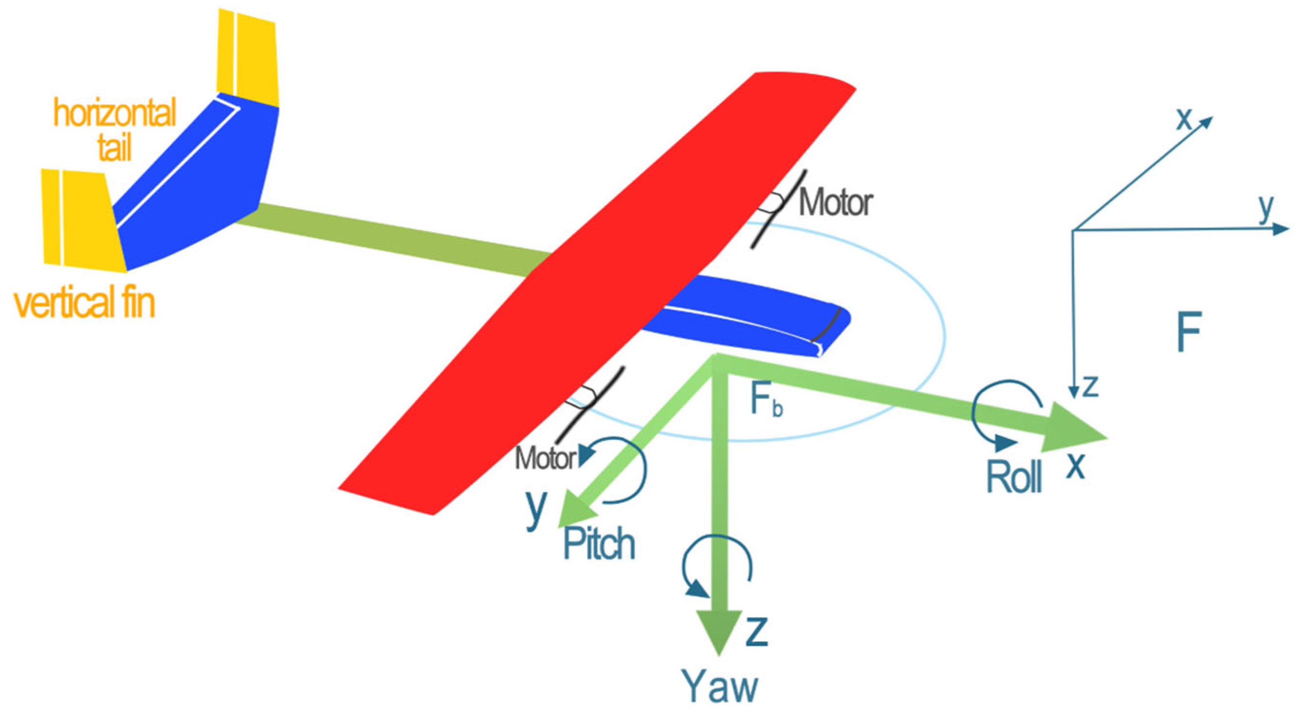
2.3. Fixed-Wing UAV Dynamic Modeling

This paper initially establishes the coordinate system for fixed-wing UAVs, as shown in Figure 1. The kinematic equations for the position, ground speed, and heading angle are relative to the inertial coordinate system, while the aircraft’s motion and aerodynamic interactions are described through the body coordinate system. The fixed-wing UAV coordinate system, as illustrated in Figure 1, includes $F_i\left(i, j, k\right)$ as the inertial reference frame, with its origin typically at the UAV’s home point (usually the takeoff point), and the unit vectors $i, j$, and k pointing toward Earth’s north and east and toward the center of the Earth, respectively. Fb $\left(x, y, z\right)$ represents the body coordinate system. The origin is at the UAV’s center of mass, with $x$ and $y$ pointing along the UAV’s longitudinal and lateral axes, and $z$ being the axis perpendicular to the $\left(x, y\right)$ plane, pointing downward. $\gamma$ is for the roll angle, $\theta$ for the pitch angle, $\lambda$ for the yaw angle, and $\left(x, y, z\right)$ represents the position of the centroid in an inertial coordinate system.

$$\begin{array}{c}{R}_i^b=R(\gamma )R(\theta )R(\lambda )\\ =\left(\begin{array}{ccc}1& 0& 0\\ 0& \cos \gamma & \sin \gamma \\ 0& -\sin \gamma & \cos \gamma \end{array}\right)\left(\begin{array}{ccc}\cos \theta & 0& -\sin \theta \\ 0& 1& 0\\ \sin \theta & 0& \cos \theta \end{array}\right)\left(\begin{array}{ccc}\cos \lambda & \sin \lambda & 0\\ -\sin \lambda & \cos \lambda & 0\\ 0& 0& 1\end{array}\right)\\ =\left(\begin{array}{ccc}{c}_{\theta }{c}_{\lambda }& c_{\theta }{s}_{\lambda }& -s_{\theta }\\ s_{\gamma }{s}_{\theta }{c}_{\lambda }-c_{\gamma }{s}_{\lambda }& s_{\gamma }{s}_{\theta }{s}_{\lambda }+c_{\gamma }{c}_{\lambda }& s_{\gamma }{c}_{\theta }\\ c_{\gamma }{s}_{\theta }{c}_{\lambda }+s_{\gamma }{s}_{\lambda }& c_{\gamma }{s}_{\theta }{s}_{\lambda }-s_{\gamma }{c}_{\lambda }& c_{\gamma }{c}_{\theta }\end{array}\right)\end{array}$$

(1)

Next, this paper defines 12 state quantities of fixed-wing UAVs, namely, three position states $(P^n,P^e,P^d)$; the three velocities correspond to translational motion $(o,v,a)$. Three angular displacements and three angular velocities correspond to rotational motion $(p,q,r)$. Note that this is defined here as the angular velocity, not the Euler angular rate, that is, not equal to the time derivative of the Euler Angle; height $h=-p_d$.

$$\left(\begin{array}{l}{\dot{p}}_n\hfill \\ {\dot{p}}_e\hfill \\ {\dot{p}}_d\hfill \end{array}\right)={\left(\begin{array}{ccc}{c}_{\theta }{c}_{\lambda }& c_{\theta }{s}_{\lambda }& -s_{\theta }\\ s_{\gamma }{s}_{\theta }{c}_{\lambda }-c_{\gamma }{s}_{\lambda }& s_{\gamma }{s}_{\theta }{s}_{\lambda }+c_{\gamma }{c}_{\lambda }& s_{\gamma }{c}_{\theta }\\ c_{\gamma }{s}_{\theta }{c}_{\lambda }+s_{\gamma }{s}_{\lambda }& c_{\gamma }{s}_{\theta }{s}_{\lambda }-s_{\gamma }{c}_{\lambda }& c_{\gamma }{c}_{\theta }\end{array}\right)}^T\left(\begin{array}{l}o\hfill \\ v\hfill \\ a\hfill \end{array}\right)$$

(2)

Above is the dynamic model of the position state.

$$\left(\begin{array}{c}\dot{\gamma }\\ \dot{\theta }\\ \dot{\lambda }\end{array}\right)=\left(\begin{array}{ccc}1& \sin \gamma \tan \theta & \cos \gamma \tan \theta \\ 0& \cos \gamma & -\sin \gamma \\ 0& \sin \gamma /\cos \theta & \cos \gamma /\cos \theta \end{array}\right)\left(\begin{array}{l}p\hfill \\ q\hfill \\ r\hfill \end{array}\right)$$

(3)

Above is the dynamic model of three angular displacements.

$$\left(\begin{array}{c}\dot{o}\\ \dot{v}\\ \dot{a}\end{array}\right)=\left(\begin{array}{c}rv-qa\\ pa-ro\\ qo-pv\end{array}\right)+\frac{1}{m}\left(\begin{array}{c}{f}_x\\ f_y\\ f_z\end{array}\right)$$

(4)

Above is the model of three velocity dynamics.

$$\left(\begin{array}{c}\dot{p}\\ \dot{q}\\ \dot{r}\end{array}\right)=\left(\begin{array}{c}{\mathrm{\Gamma }}_{1}pq-{\mathrm{\Gamma }}_{2}qr+{\mathrm{\Gamma }}_{3}l+{\mathrm{\Gamma }}_{4}n\\ {\mathrm{\Gamma }}_{5}pr-{\mathrm{\Gamma }}_6\left(p^2-r^2\right)+\frac{1}{J_y}m\\ {\mathrm{\Gamma }}_{7}pq-{\mathrm{\Gamma }}_{1}qr+{\mathrm{\Gamma }}_{4}l+{\mathrm{\Gamma }}_{8}n\end{array}\right)$$

(5)

Above is the dynamic model corresponding to the three angular velocities, where m is the mass of the body, and f is the external force.

$$\begin{array}{l}{\mathrm{\Gamma }}_1=\frac{J_{xz}\left(J_x-J_y+J_z\right)}{\mathrm{\Gamma }},{\mathrm{\Gamma }}_2=\frac{J_z\left(J_z-J_y\right)+J_{xz}^2}{\mathrm{\Gamma }},\\ {\mathrm{\Gamma }}_3=\frac{J_z}{\mathrm{\Gamma }},{\mathrm{\Gamma }}_4=\frac{J_{xz}}{\mathrm{\Gamma }},{\mathrm{\Gamma }}_5=\frac{J_z-J_x}{J_y},{\mathrm{\Gamma }}_6=\frac{J_{xz}}{J_y},\\ {\mathrm{\Gamma }}_7=\frac{\left(J_x-J_y\right)J_x+J_{xz}^2}{\mathrm{\Gamma }},{\mathrm{\Gamma }}_8=\frac{J_x}{\mathrm{\Gamma }}\end{array}$$

(6)

where $p_n$ is the displacement in the $i^i$ direction ($F^i$ inertial system), $p_e$ is the displacement in the $j^i$ direction ($F^i$ inertial system), $p_d$ is the displacement in the $k^i$ direction ($F^i$ inertial system), $o$ is the displacement in the $i^b$ direction ($F^b$ inertial system), $v$ is the displacement in the $j^b$ direction ($F^b$ inertial system), $a$ is the displacement in the $k^b$ direction ($F^b$ inertial system), $\gamma$ is the roll angle, $\theta$ is the pitch angle, $\lambda$ is the yaw Angle, $p$ is the rotation rate in roll $i^b(F^{b}inertial system)$, $q$ is the pitch angle velocity $j^b(F^{b}inertial system)$, and $r$ is the yawing rate $k^b{F}^b(inertial system)$.

Of course, the above dynamic model assumes that the inertial system of the ground is on the horizontal ground, ignoring the rotation of the Earth and ignoring the external forces. Next, the forces and torques generated by the external forces of the model are established.

The aerodynamic model of the gravity is as follows:

$$f_g^b={\mathcal{R}}_v^b\left(\begin{array}{c}0\\ 0\\ mg\end{array}\right)=\left(\begin{array}{c}-mg\sin \theta \\ mg\cos \theta \sin \gamma \\ mg\cos \theta \cos \gamma \end{array}\right)$$

(7)

The aerodynamic model of the lift is as follows:

$$F_{lift}=\frac{1}{2}\rho V_a^{2}S\left[C_{Io}+C_{Ie}\alpha +C_{Iq}\frac{c}{2V_{\alpha }}q+C_{I_{\delta \epsilon }}{\delta }_e\right]$$

(8)

The aerodynamic model of the drag is as follows:

$$F_{\mathrm{drag} }\approx \frac{1}{2}\rho V_a^{2}S\left[C_{To}+C_{Te}\alpha +C_{Tq}\frac{c}{2V_{\alpha }}q+C_{T_{\delta e}}{\delta }_e\right]$$

(9)

The aerodynamic model of the pitching force is as follows:

$$M=\frac{1}{2}\rho V_a^{2}Sc\left[C_{Z\mathrm{o}}+C_{Ze}\alpha +C_{Zq}\frac{c}{2V_{\alpha }}q+C_{Z_{\delta e}}{\delta }_e\right]$$

(10)

where $S$ is the wing area; c is the average aerodynamic chord of the wing; $\rho$ is the density of the air; $\alpha$ is the angle of the attack; $q$ is the rotation rate in the pitch; ${\delta }_e$ is the elevator; $C_{Io},C_{Ie},C_{Iq},C_{I_{\delta \epsilon }}$ are dimensionless lift coefficients; $C_{To},C_{Te},C_{Tq},C_{T_{\delta e}}$ are dimensionless drag coefficients; and $C_{Z\mathrm{o}},C_{Ze}\alpha ,C_{Zq},C_{Z_{\delta e}}$ are dimensionless moment coefficients.

The above three equations are the longitudinal aerodynamic model for the case of small angles of attack, and similarly, the transverse dynamic model can be expressed as follows:

$$\left\{\begin{array}{c}{f}_y\approx \frac{1}{2}\rho V_a^{2}S\left[C_{Y_O}+C_{Y_{\beta }}\phi +C_{Y_p}\frac{b}{2V_a}R+C_{Y_s}\frac{b}{2V_a}r+C_{Y_{{\delta }_r}}{\delta }_r\right]\\ k\approx \frac{1}{2}\rho V_a^{2}Sb\left[C_{lo}+C_{l_{\beta }}\phi +C_{l_p}\frac{b}{2V_a}R+C_{l_s}\frac{b}{2V_a}r+C_{l_{{\delta }_r}}{\delta }_r\right]\\ n\approx \frac{1}{2}\rho V_a^{2}Sb\left[C_{no}+C_{n_{\beta }}\phi +C_{n_p}\frac{b}{2V_a}R+C_{n_s}\frac{b}{2V_a}r+C_{n_{{\delta }_r}}{\delta }_r\right]\end{array}\right.$$

(11)

$$\left\{\begin{array}{c}{f}_y\approx \frac{1}{2}\rho V_a^{2}S\left[C_{Y_O}+C_{Y_{\beta }}\phi +C_{Y_p}\frac{b}{2V_a}\gamma +C_{Y_s}\frac{b}{2V_a}r+C_{Y_{{\delta }_r}}{\delta }_r\right]\\ k\approx \frac{1}{2}\rho V_a^{2}Sb\left[C_{lo}+C_{l_{\beta }}\phi +C_{l_p}\frac{b}{2V_a}\gamma +C_{l_s}\frac{b}{2V_a}r+C_{l_{{\delta }_r}}{\delta }_r\right]\\ n\approx \frac{1}{2}\rho V_a^{2}Sb\left[C_{no}+C_{n_{\beta }}\phi +C_{n_p}\frac{b}{2V_a}\gamma +C_{n_s}\frac{b}{2V_a}r+C_{n_{{\delta }_r}}{\delta }_r\right]\end{array}\right.$$

(12)

where $\phi$ is the side slip angle, $R$ is the roll angle, $r$ is the yawing rate, ${\delta }_r$ is the rudders, $f_y$ is the lateral force, $k$ is the rolling moment, $n$ is the yaw moment, and $C_{*}$ is the aerodynamic coefficient.

The thrust produced by the propeller is

$$f_p=\frac{1}{2}\rho S_{\mathrm{prop} }{C}_{\mathrm{prop} }\left(\begin{array}{c}{\left(p_{\mathrm{motor} }{\delta }_t\right)}^2-V_a^2\\ 0\\ 0\end{array}\right)$$

(13)

where $p_{motor}$ is the transmission efficiency coefficient of the motor, and the propeller sweep area is $S_{\mathrm{prop}}$. The atmospheric disturbance can be expressed as follows:

$$V_w=\left(\begin{array}{c}{w}_o\\ w_e\\ w_c\end{array}\right)V_{w_s}^i=\left(\begin{array}{l}{w}_{o_s}\hfill \\ w_{e_s}\hfill \\ w_{c_s}\hfill \end{array}\right)V_{w_s}^b=\left(\begin{array}{l}{y}_{w_g}\hfill \\ v_{w_g}\hfill \\ w_{w_g}\hfill \end{array}\right)$$

(14)

where $V_{w_s}$ is the value of the airflow velocity in a stable environment; $v_{w_g}$ is the airflow disturbance value; $w_{o_s},w_{e_s},w_{c_s}$ are the steady-state airflow velocity values pointing north, east, and to the center of the Earth, respectively; and $y_{w_g},v_{w_g},w_{w_g}$ are the velocity components of the turbulent airflow pointing north, east, and geocentric.

According to the kinetic equation in this study [45], a robust controller is designed, and the control rate formula is as follows:

$$u={\ddot{y}}_d-h_1{e}_1-h_0{e}_0-\widehat{d}-k_d{\dot{x}}_2$$

(15)

In this formula, the robust control rate is mainly composed of three parts: $({\ddot{y}}_d-h_1{e}_1-h_0{e}_0)$, a proportional controller; $\widehat{d}$, the observers; and $k_d{\dot{x}}_2$, the forecasts. The parameters of the control rate depend on the order of the system; for example, the roll control system is a second-order system, and parameters $h_1,h_0$ guarantee that the spectrum of the polynomial, $h(s)=h_0=h_{1}s$, is distributed in the left half-plane; $k_d$ is nonnegative constant, $e_0=y-y_d$.

2.4. Wing Design

2.4.1. Wing Shape and Function

First, in the wing shape selection, the preliminary selection between CLARK Y and NACA 4412, two kinds of planoconvex wings, Re = 250,000 under the CLARK Y and NACA 4412 lift and drag characteristics, as shown in Figure 2. The black line represents the characteristic curve of the NACA 4412 wing. The blue line represents the characteristic curve of the CLARK Y airfoil. Combined with the lift-to-drag ratio characteristic curve, as shown in Figure 3. The black lines also represent the lift-to-drag characteristic curve of the NACA 4412 airfoil. The blue line represents the lift to drag characteristic curve of the CLARK Y airfoil. It can be seen that for the NACA 4412 in the same headway angle under the lift, the coefficient is higher, and the lift-to-drag ratio characteristics are also better. Combined with NACA 6409 and NACA 6412, although the lift coefficient is higher, the critical stall angle is too small; the drag and fabrication are more difficult, and the extreme load capacity is not needed for the ground. Moreover, because of the choice of the trapezoidal wing, the effective angle of the wing profile increases toward the wingtip, and the separation occurs first in the wingtip, which reduces the aileron rudder maneuvering. Thus, the critical stall angle is preferred. Therefore, the airfoil with a larger stall critical angle is preferred, and the planoconvex NACA 4412 airfoil is selected.

The shape of the wing designed in this study is [9] shown in Figure 4, which has the following main features:

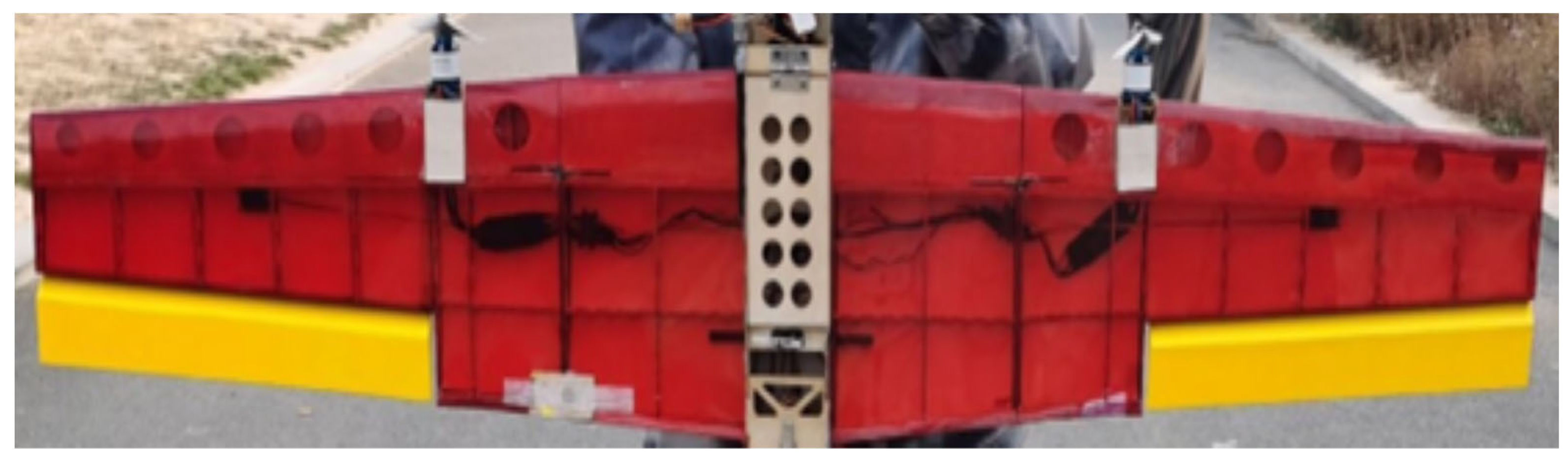
• A trapezoidal planar wing is used; this shape is simple and practical, suitable for low- and medium-speed flights, and easy to manufacture and install;
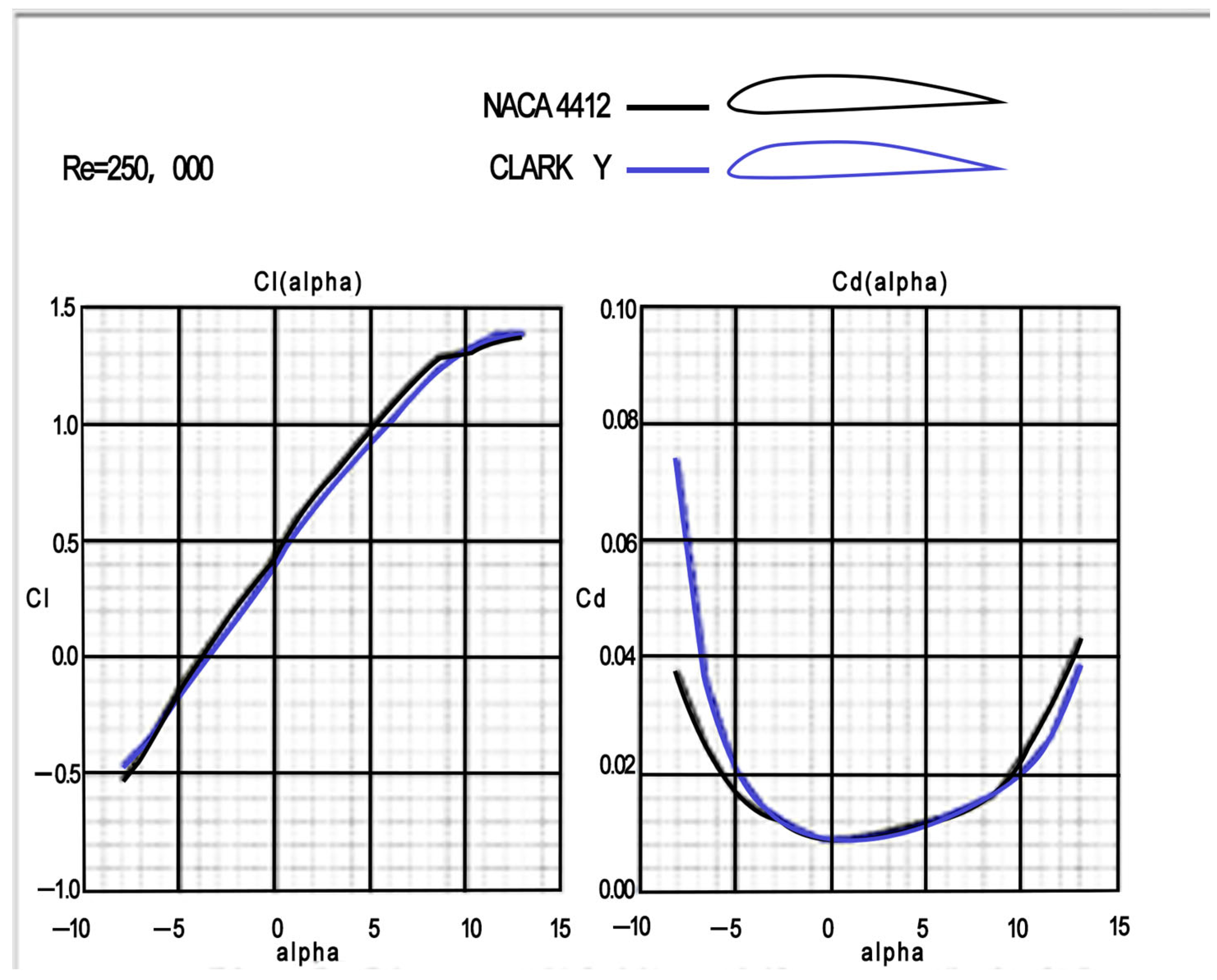
• NACA 4412 is chosen as the wing model, which has a high lift coefficient and low drag coefficient and is suitable for low- and medium-speed flights, as well as under takeoff and landing and stall conditions;
• The wing sweep angle is designed as 3°; this camber can reduce the induced drag of the wing and improve the lateral stability and maneuverability of the aircraft.

2.4.2. Relationship between Wing Parameters and Performance

Wing parameters are crucial determinants of wing performance, with varying parameters exerting distinct impacts. Referring to aircrafts within the same Reynolds number range, the wing loading is preliminarily set at 65 g/dm², from which the wing area is deduced to be 3400 cm², and the wingspan is 150.22 cm. A single wing side is chosen to be 70 cm, resulting in a wingspan of 148.7 cm (with the fuselage width being 8.7 cm), an aspect ratio of 6.87, and a taper ratio selected at 1.5, meaning that the wing root is 276 mm, and the wingtip is 184 mm, with a sweep angle of 3°. Given the wing’s mounting position near the topmost part of the fuselage, the stability is enhanced; thus, we do not set an opposite angle. The aileron area is initially set to 20% of the wing area. Considering folding mechanisms, the final aileron length is 420 mm, with a chord length of 68 mm, accounting for approximately 17.8% of the wing area. The principal parameters are detailed in

Table 3. Main parameters of the wing.

L/mm	b0/mm	b1/mm	MAC/mm	λ	av	Sweep Angle/°
1487	276	184	233	6.87	1.5	3

.

The wing design parameters articulated in this study, as enumerated in

Table 4. Main parameters of the tail wing.

	Tail Arm/mm	Tail Capacity	Area/mm2	Sweep Angle/°
Horizontal tail	550	0.67	85,000	6
Vertical tail		0.05	22,000 × 2	25

, exert several significant effects.

A wingspan of 1487 mm was selected, based on an integrated consideration of the UAV’s design requisites and flight performance, to ensure adequate lift while minimizing the drag and weight.

The UAV design employs a chord length of 233 mm, as determined by balancing the UAV’s load demands and structural integrity, thus providing sufficient lift while ensuring the wing’s strength and rigidity.

An aspect ratio of 6.87 was chosen, aiming to optimize the UAV’s flight velocity and efficiency, thereby enhancing the lift-to-drag ratio and glide ratio while controlling wing deformation and buckling.

A taper ratio [46] of 1.50 was selected, considering the balance between the UAV’s aerodynamic performance and stability, capable for lowering the drag coefficient while maintaining adequate lateral stability.

To accommodate the UAV’s flight speed and control requirements, a sweep angle of 3° was chosen, effectively reducing induced drag while ensuring sufficient lateral stability and maneuverability.

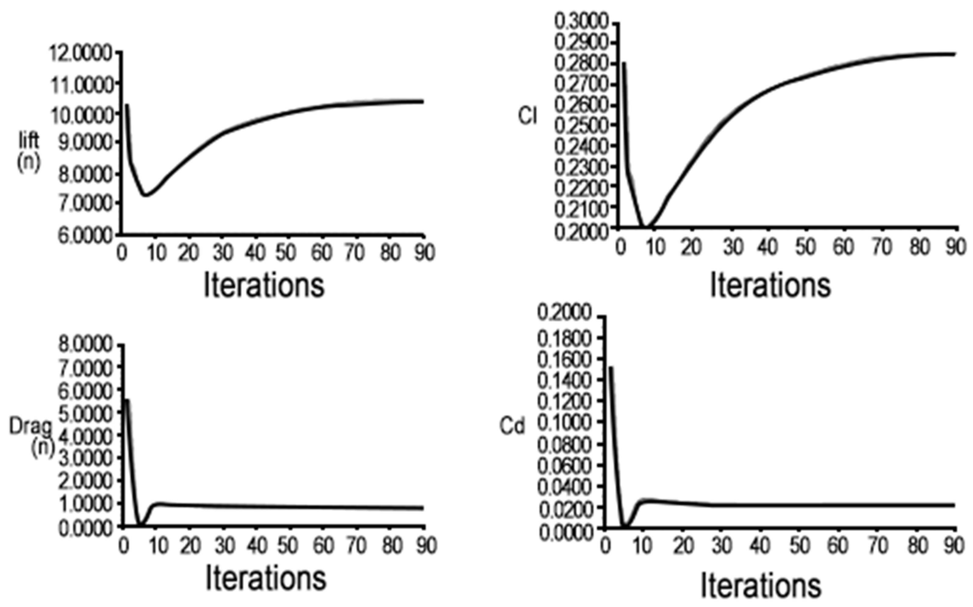
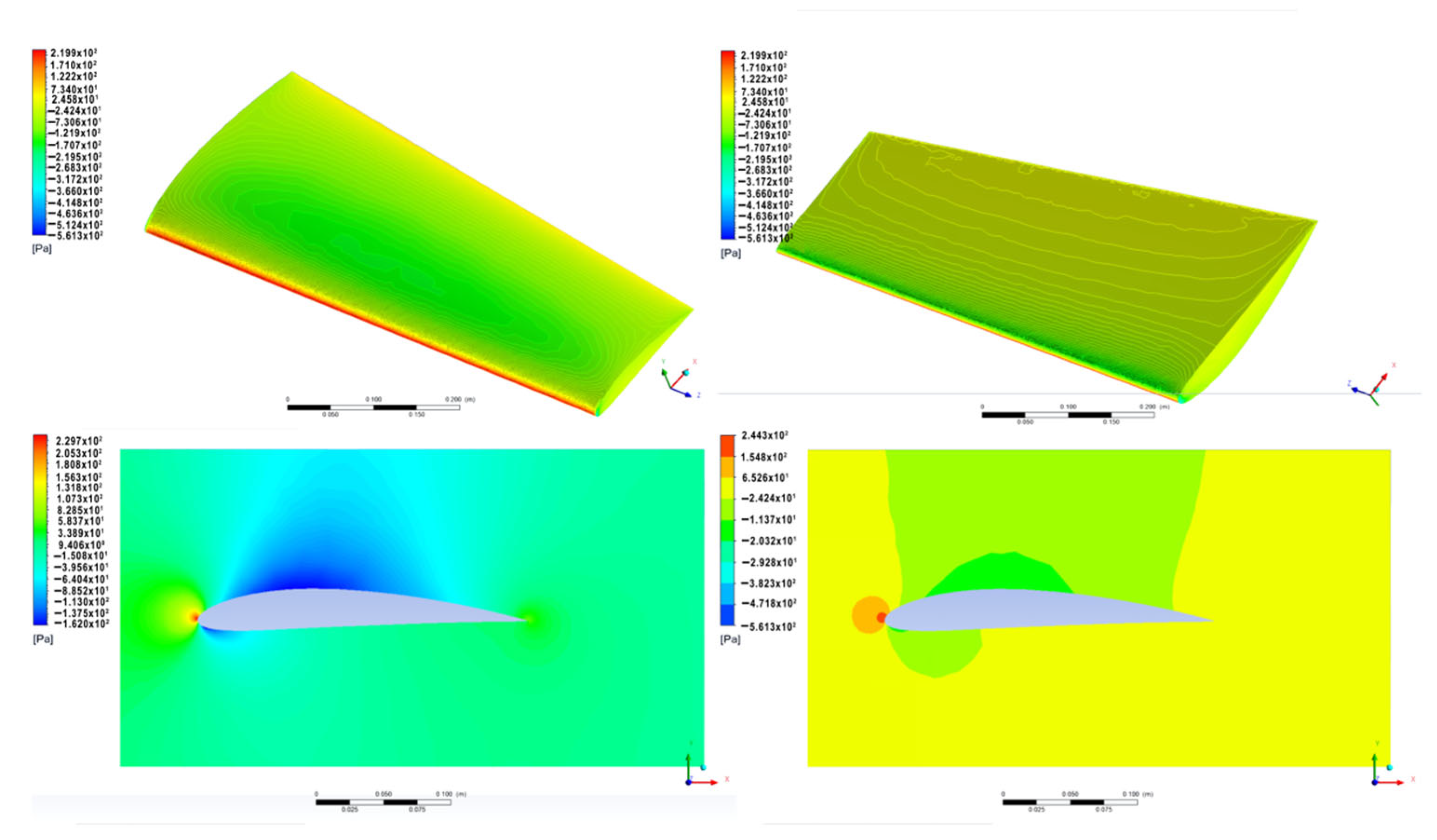
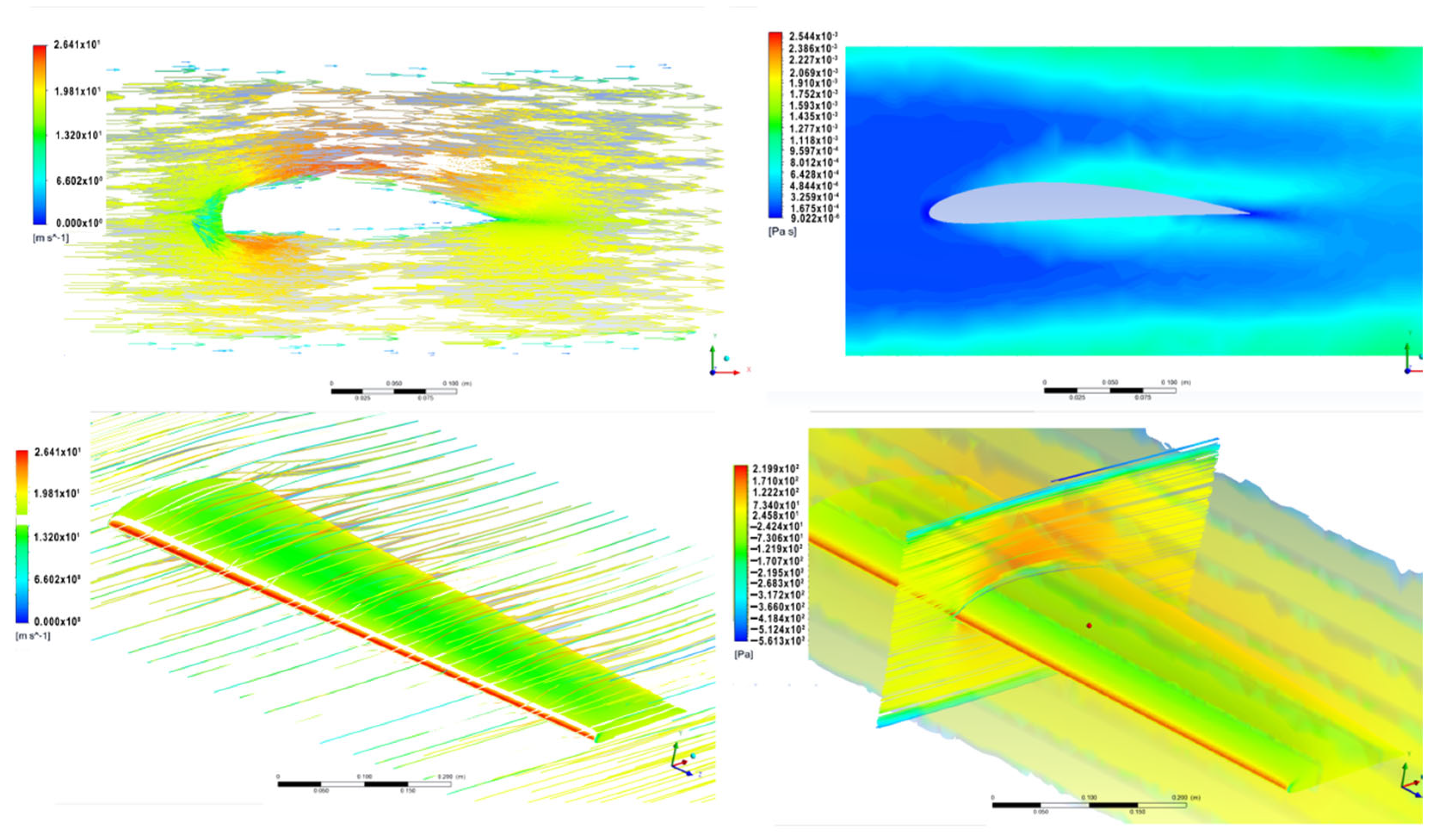
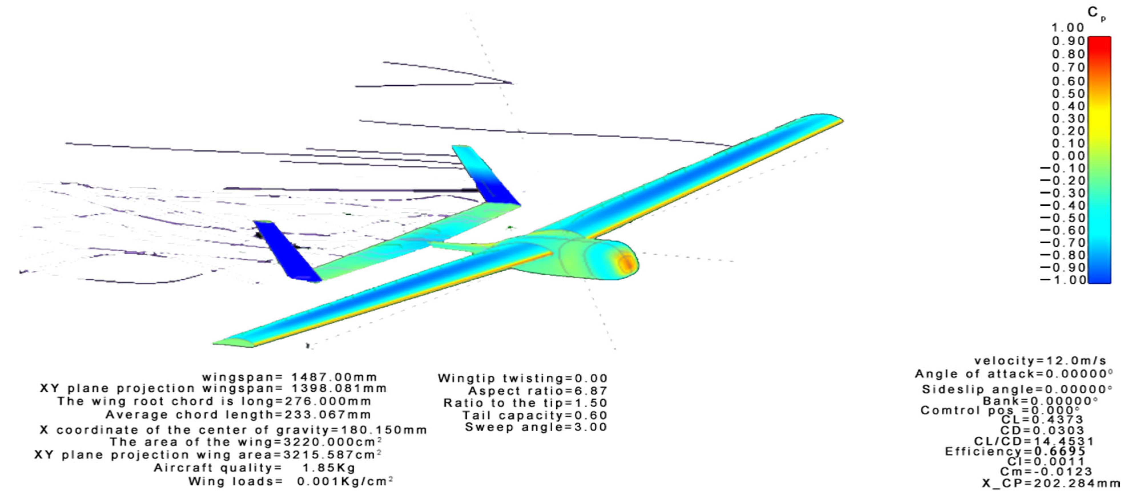
2.4.3. Analysis of Wing Aerodynamics

The aerodynamic analysis of the wing can enhance aircraft performance [47].

Initially, this study conducts a preliminary mesh division of the wing model, considering practical engineering applications, and adopts tetrahedral meshing. By ensuring reasonable computational accuracy, this study reduces the number of meshes, ultimately setting the mesh size to approximately 15 mm. The results are displayed in Figure 5.

Upon completing the preprocessing, this study proceeds to a solution using Fluent, deciding to position the wing within a flow field having an inlet and outlet area of 0.3083 square meters for computations. Taking into account the designated cruising speed of the flight platform and the typical wind speeds in the flight test area, the inlet airspeed is set at 19 m/s. When Fluent is used for iteration, the convergence curve gradually flattens out and approaches the steady state after 100 iterations. Meanwhile, to save computing resources, 100 is selected as the number of iterations. Although convergence to 0.001 was not achieved, it is close to the steady state and can be ignored. The computational outcomes are illustrated in Figure 6. The black area represents the core part of the wing, an internal structure or high-density mesh area for more accurate calculations and analysis. The blue area represents the meshing of the wing surface, which is a tetrahedral mesh. This part of the mesh is relatively sparse and is mainly used for large-scale hydrodynamic calculations to ensure the accuracy of the calculation while reducing the number of meshes.

As illustrated in the figure, with the increasing continuity of the iteration numbers, the velocity in various directions and other parameters tend to stabilize. This study also establishes how the wing’s lift, lift coefficient, drag, and drag coefficient change as the number of iterations increases.

As depicted in Figure 7, the top left shows the wing’s lift curve, the top right displays the wing’s lift coefficient curve, the bottom left illustrates the wing’s drag curve, and the bottom right presents the wing’s drag coefficient curve. Based on the computational results, it can be concluded that the wing generates relatively high lift and incurs low drag at the planned cruising speed. This indicates that the initially chosen airfoil and determined parameters, such as the chord length, wingspan, and taper ratio, are well suited to the requirements of our flight.

After completing the iteration calculations, this study proceeds with post-processing of the wing’s flow field simulation, as shown in Figure 8. This process also yields several noteworthy analytical results, as discussed below.

The figure illustrates the static pressure distribution on the wing surface (top left and top right for the upper/lower surfaces). The pressure on the upper and lower surfaces of the wing is relatively low and evenly distributed. This analysis suggests that during the manufacturing of the leading edge, attention should be paid to enhance its stiffness, and the rational distribution of wing ribs in terms of quantity and material should be considered. Additionally, applying carbon patches near the wingtips may prevent bending at the wing edges.

The bottom-left and bottom-right images show the local and overall pressure distributions, respectively. From these images, it is determined that the actual aerodynamic pressure effects in the external flow field are essentially consistent with the static pressure analysis results.

As shown in Figure 9, the wing achieves its maximum lift-to-drag ratio at an angle of attack of 2°, with CL/Cd = 17.38. The lift generated at this point is substantial, fully satisfying the requirements for the stable flight of the platform. Consequently, a wing installation angle of 2° is chosen.

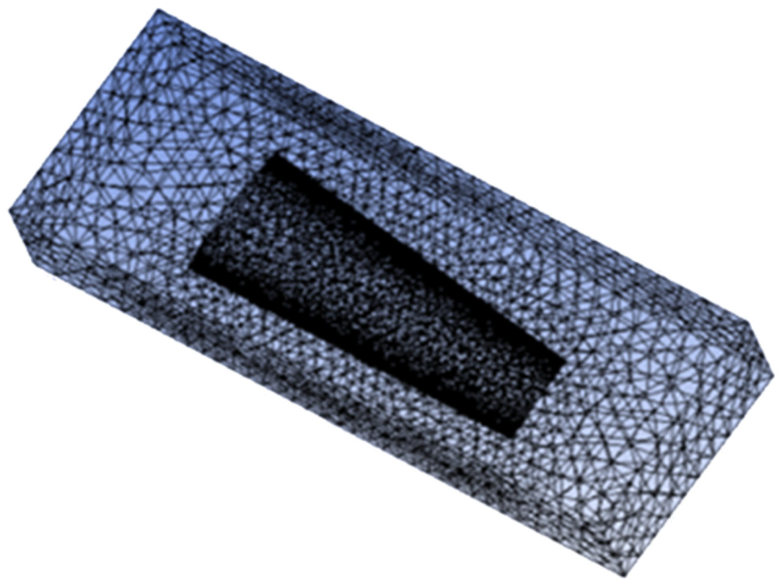
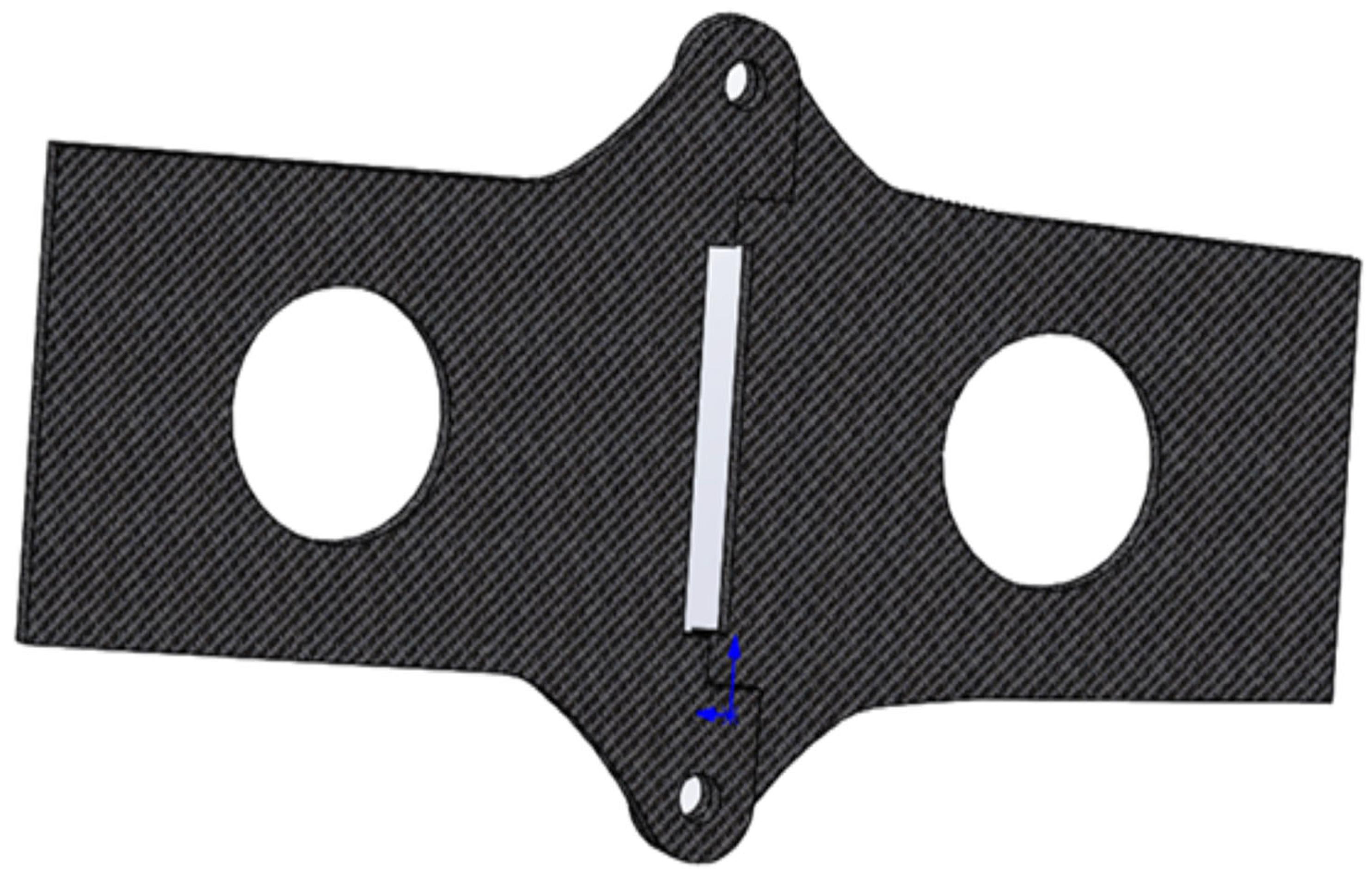
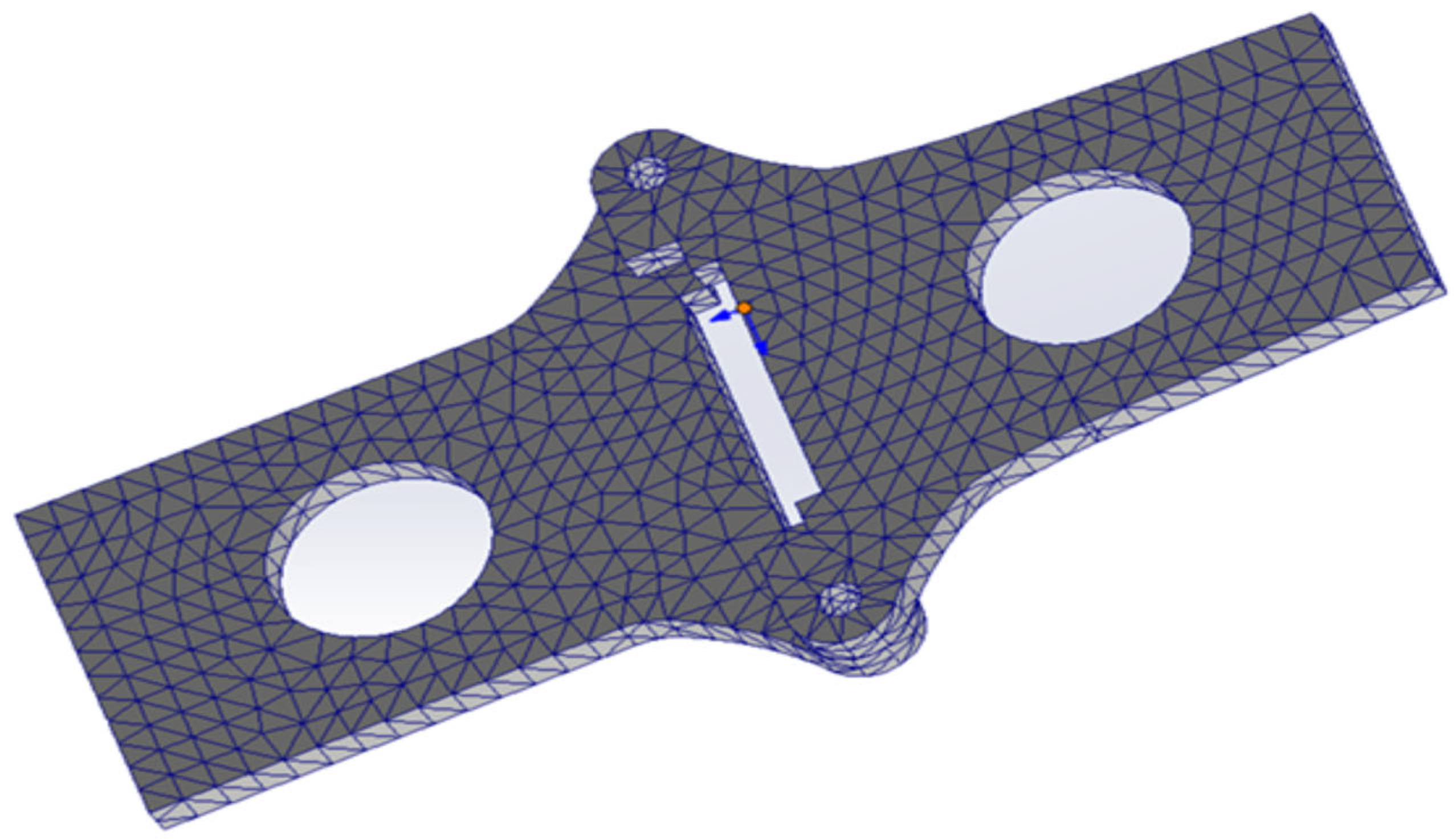
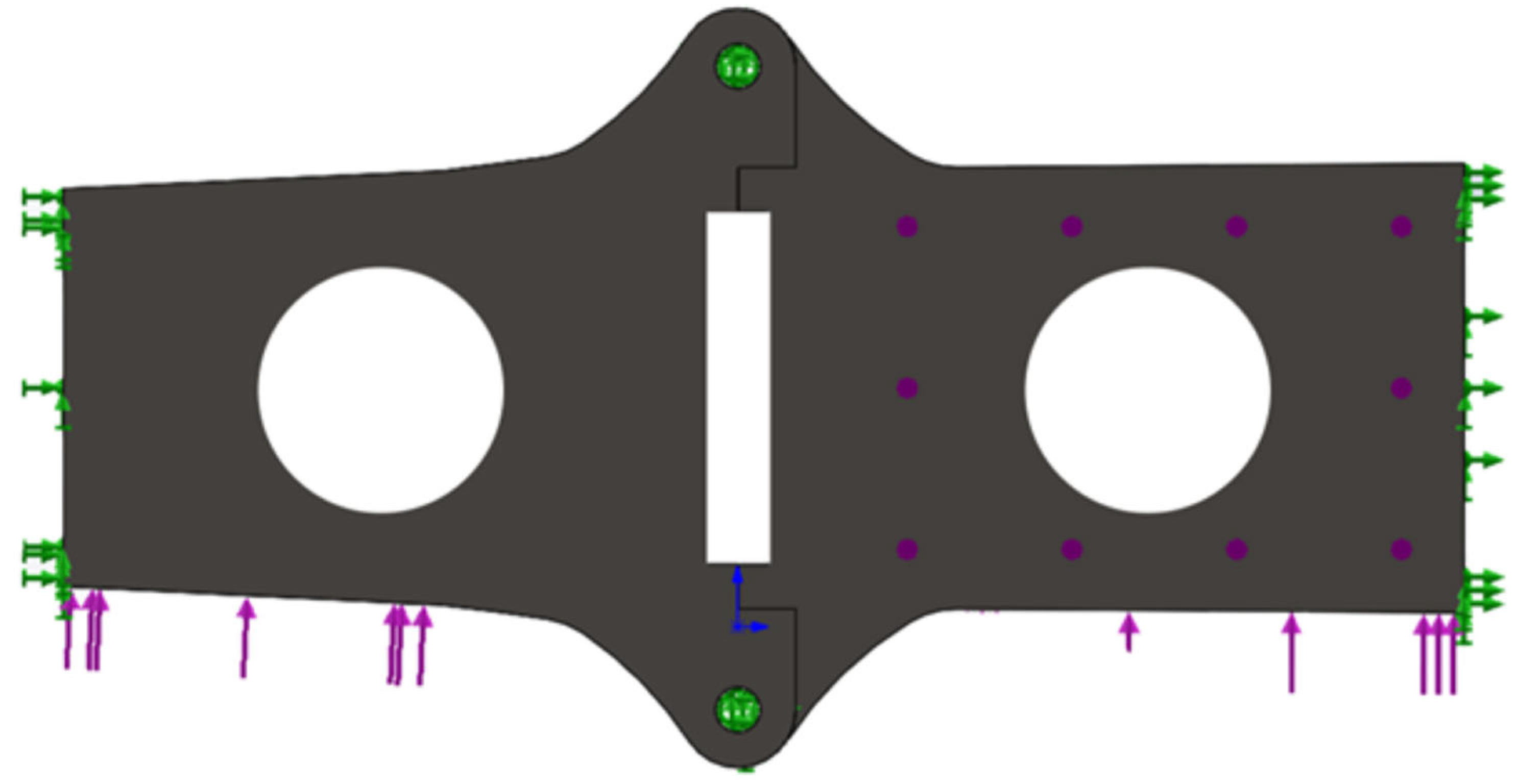
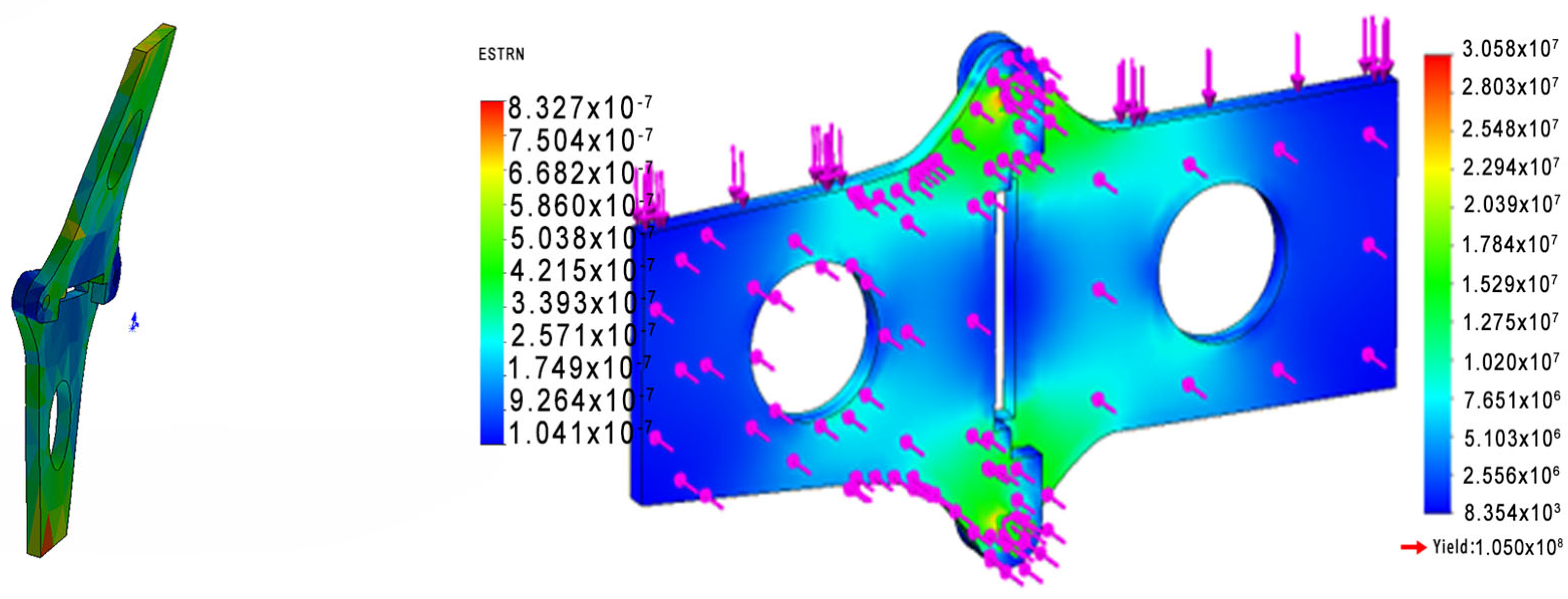
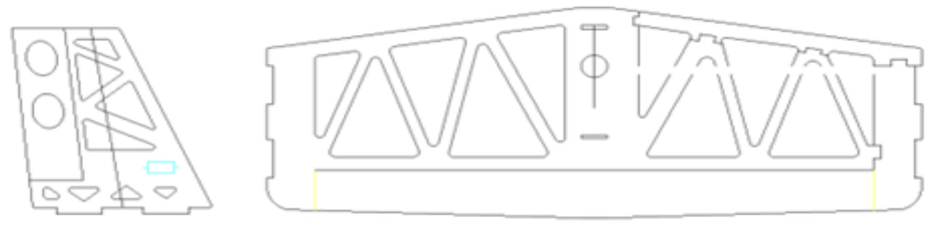
2.4.4. Finite Element Analysis of Outer Wing and Middle Wing Connector

To save space and enhance portability, this study designs the UAV with foldable wings, dividing the wing into the midsection and outer sections. The midsection is directly fixed to the fuselage, while the outer sections are equipped with propulsion systems. To prevent risks such as mid-air disassembly, it is crucial to analyze the strength and stability of the connector under the aerodynamic loads on the wings. The three-dimensional model of the connector is imported into finite element analysis software, and the model undergoes a geometric cleanup. As shown in Figure 10, the connector consists of two parts, each fixed to the spar of the midsection and outer sections of the wing. Once the left and right parts of the connector are joined, bolts are used to secure the upper and lower holes.

Subsequently, the geometric model of the connector undergoes finite element mesh division, as illustrated in Figure 11.

This study employs carbon fiber plates for wing connectors, defined in finite element software for stress testing. During flights, these connectors face lift and aerodynamic forces, with simulated loads applied to model the wing-generated lift in the analysis, as illustrated in Figure 12.

Through the static analysis of the middle wing and the outer wing, the deformation and stress programs of the connecting parts are obtained, as shown in Figure 13.

Connectors made of 2 mm carbon fiber plates are lightweight but possess high strength. As indicated by the stress analysis, deformation can occur in the connectors. To meet the wing strength requirements of this study, we enhance the strength at the junction between the connectors and the wing spars to prevent the deformation of the connectors.

2.5. Design of the Tail and Fuselage [48]

2.5.1. Determination of the Role and Parameters of the Tail Wing

As shown in Figure 14, twin vertical stabilizers enhance the vertical and directional stability [49,50], reduce airframe oscillation, and improve handling by increasing the surface area and yaw control efficiency. This study adopts a dual vertical H-shaped tail design and uses carbon tubes to connect the fuselage. Because of the use of advanced flight control technology, the tail volume coefficient is reduced by 10% to 15% compared with similar aircrafts. The horizontal tail volume is set at 0.6, with an average chord length of 170 mm and a span of 500 mm. The horizontal tail volume coefficient, CHT = LHTSHT/CWSW, is calculated to be 0.6, resulting in a tail arm length, LHT, of 521 mm. To maximize the folding space, the final tail arm length is set at 550 mm, resulting in CHT = 0.67, with a wing sweep angle of 3° to ensure the horizontal tail stalls after the wing, minimizing airflow interference from the main wing to the tail. The horizontal tail’s sweep angle is set at 6°, and the horizontal tail is mounted at approximately 30°. The vertical tail volume is set at 0.05, with a sweep angle of 25°. Based on the calculation CVT = LVTSVT/bWSW, the single vertical tail area is approximately 22,000 mm². The elevator is designed to occupy 20% of the horizontal tail area and the rudder to occupy 25% of the vertical tail area. Table 4 illustrates the primary parameters of the tail configuration. The design drawings of the tail are shown in Figure 15.

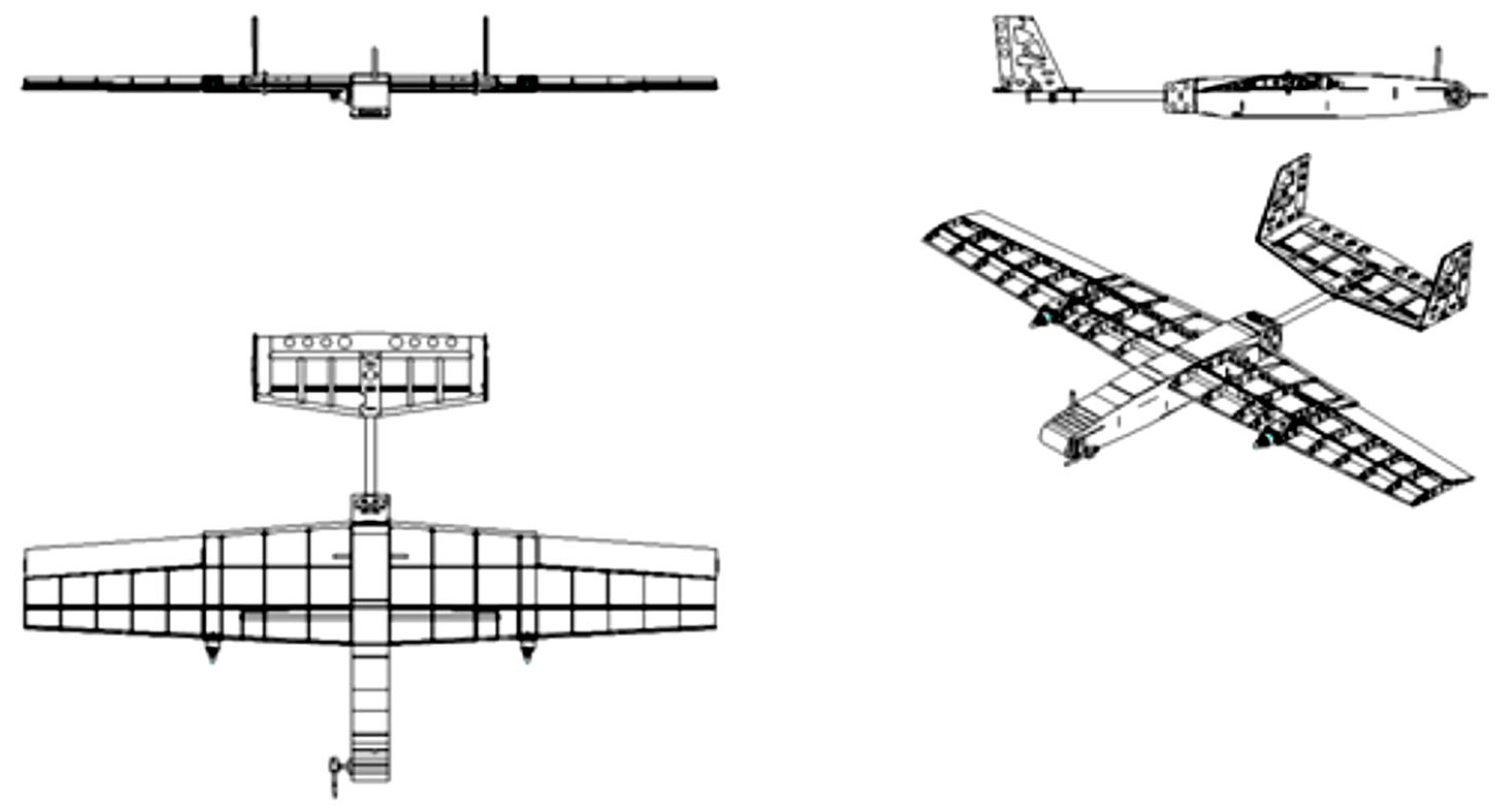
2.5.2. Fuselage Design

The aerodynamically designed fuselage, with an upward-tilting nose to protect the camera, uses dual motors for CG balancing and features a slender, reinforced structure with bulkheads and carbon tubes for enhanced torsional resistance and bending moment management, as detailed in

Table 5. Fuselage parameter.

Overall Length/mm	Maximum Height/mm	Width/mm	Magazine Length/mm
655	97	80	182

and illustrated in Figure 16’s complete aircraft aerodynamic analysis using Fluent.

Because of the adoption of a twin-engine, single-wing H-tail configuration, the stability is favorable, and the turning radius is reduced to a reasonable range because of the advantage of the differential thrust from the twin engines. Utilizing a high-aspect-ratio trapezoidal wing, the wing loading reaches approximately 65 g/dm² under full mission payload conditions. Employing the NACA 4412 symmetrical airfoil necessitates a certain manual launch acceleration at takeoff. Regarding the payload capacity, tests have shown that even when equipped with a GoPro 6 and an additional 100 g of weight, it can still takeoff with the mission payload, although the climb rate is low, prompting an increase in the motor’s down-angle by 1° in later stages. Simulating logistic delivery missions, the UAV uses a 500 mL water bottle to mimic small-volume items. Under light wind conditions, through multiple tests, the accuracy of the delivery to the target area is within a 3 m range.

2.6. Design of Main Parameters

The three most crucial parameters for an aircraft are the wing area, S $({\mathrm{m}}^2)$, the takeoff weight of the aircraft, $m_0$ (kg), and the static thrust of the power unit, $P_o\left(dan,1dan=10^{-5}\mathrm{N}\right)$. The corresponding parameters are

$$P_{O=}\frac{m_{o}g}{10S}\left(\mathrm{dan}/{\mathrm{m}}^2\right)$$

(16)

The above equation is the formula for calculating the load of the starting wing.

$$v_{\mathrm{m}\mathrm{a}\mathrm{x}}=10P/\left(m_{o}g\right)$$

(17)

The above formula is the common formula for calculating the takeoff thrust-to-weight ratio.

The maximum takeoff weight of the UAV in this article is 2 kg; the thrust of the selected brushless motor is 1.47 kg, and the wing area is 3400 $\mathrm{c}{\mathrm{m}}^2$. From this, it can be calculated that the maximum wing load at takeoff is 65 $\mathrm{g}/\mathrm{d}{\mathrm{m}}^2$, and the takeoff thrust-to-weight ratio is 1.5.

1.

Lift–drag ratio

(1)

Lift and lift coefficient

According to Bernoulli’s theorem, the amount of lift generated by an airfoil can be calculated using the following formula:

$$L=\frac{1}{2}\rho V^{2}S{C}_L$$

(18)

where L is the lift force (N), $\rho$ is the air density ($\mathrm{k}\mathrm{g}/{\mathrm{m}}^3$), V is the relative velocity (m/s), S is the wing area (${\mathrm{m}}^2$), and C_L is the wing’s lift coefficient.

  (2)

Drag and drag coefficient

The resistance formula is

$$D=\frac{1}{2}\rho V^{2}S{C}_D$$

(19)

where D is the drag force (N), $\rho$ represents the air density ($\mathrm{k}\mathrm{g}/{\mathrm{m}}^3$), V is the relative velocity (m/s), S is the wing area (${\mathrm{m}}^2$), and C_D is the coefficient of lift for the wing.

From (3) and (4), it can be seen that the lift-to-drag ratio of the aircraft is $\frac{C_L}{C_D}$.

2.

Service ceiling (Hmax)

The practical ceiling refers to the maximum flight altitude at which an aircraft can maintain a level flight state under human operation, and the magnitude of Hmax can be determined using the relative air density value at this altitude [51]. It can be derived according to the equations “weight = lift” and “thrust = drag” when the aircraft is in a level flight. Using polar curves, $C_x=C_{x0}+D_0{C}_y^2$, the following can be obtained: $K_{\max }={\left(\frac{C_y}{C_x}\right)}_{\max }=\frac{1}{2\sqrt{D_0{C}_{x0}}}$ and the rule ${\Delta }_J=\frac{1.67\sqrt{D_0{C}_{X0}}}{\xi P_0}$, where ${\Delta }_J$ is a practical ceiling. It can be seen that the practical ceiling of the aircraft is directly proportional to the thrust-to-weight ratio.

Through the above calculation formula of the aircraft performance and the basic requirements for designing UAVs, the main design parameters of UAVs are determined, as shown in

Table 6. Main UAV design parameters.

Wingspan/m	1.50	Maximum Takeoff Weight/kg	2.0
Ratio to the tip	1.50	Minimum takeoff speed m/s	10
Fuselage length/m	0.655	Maximum level-flight speed m/s	30
String span ratio	6.87	Battery life/h	0.2
Wing loads g/dm3	65	Practical ceiling/m	100
Thrust-to-weight ratio	1.5	Payload/kg	0.5

.

Figure 17 shows the top, side, and bottom views of the aircraft design, as well as some dimensional data. The aircraft has a wingspan of 1487 mm, a slender length of 233 mm, an aspect ratio of 6.87, a warp of 1.50 degrees, and a vertical tail main angle of attack of 25 degrees. The main components of the aircraft are made of balsa wood and laminate, and some of the connections are made of carbon fiber materials.

2.7. Establishment Process of Aircraft Modeling

In this study, SolidWorks software (solidworks2021) is used to conduct 3D modeling of the thrown fixed-wing UAV. The aircraft modeling process consists of the following steps: The takeoff weight of the aircraft ranges between 1900 g and 2000 g, with a flight altitude of about 30 m and a flying speed of 15 m/s. The average chord length of the wing has been preliminarily determined to be 230 mm, resulting in a Reynolds number (Re) of 235,629. A twin-engine, single-wing design with an H-tail layout is adopted, and the areas of all the control surfaces are appropriately enlarged. The combination of the flight control and an airspeed meter with a motor differential speed is used to achieve better wind resistance. Additionally, based on flying experience, reconnaissance requires a lower cruising speed. An overly heavy payload can result in poor takeoff and landing performance; hence, a high-aspect-ratio trapezoidal wing is used to increase the wing area, reduce wing loading, and induce drag while maintaining favorable lift-to-drag ratio characteristics [52,53]. Because of the low fuselage, a sponge pad is attached to the bottom of the fuselage during actual flights to increase the height and prevent the propeller blades from hitting the ground during landing. In terms of the power, to shorten mission times and provide power redundancy under strong wind conditions, the aircraft maximizes the thrust-to-weight ratio, sacrificing some endurance capabilities to achieve better climbing performance. Figure 18 shows a 3D assembly drawing of the drone.

Meanwhile, in the establishment process of the aircraft modeling, a detailed system attribute analysis of the studied fixed-wing UAV is conducted, where crucial inertial and mass properties are precisely measured and recorded. The total mass of the UAV is 1606.66 g, equipped with a payload that has a clearly defined center of gravity, with X, Y, and Z-axis coordinates at 0.01 m, 0.29 m, and −589.15 m, respectively, reflecting its balanced design and mass distribution. The inertial matrix provides critical data about the UAV’s inertial characteristics with respect to rotational motions; the principal moments of inertia are as follows: Ixx = 129,656,482.52 kg·mm², Iyy = 170,053,044.53 kg·mm², and Izz = 296,400,388.67 kg·mm², highlighting the UAV’s rotational stability along each axis. Additionally, the product of the inertia quantifies the interplay between the axes, such as Ixz = −29,702.20 kg·mm², which is crucial for understanding the UAV’s dynamic characteristics. Furthermore, the UAV design also considers additional inertial properties, such as Ixx = 853,973,205.56 kg·mm² and Izz = 130,465,594 kg·mm², to enhance its performance in various operational scenarios.

2.8. Optional Configuration of UAV Bomb-Dropping Mechanism and Power Unit

2.8.1. Power Device Selection

Because of the high efficiency and long life of the brushless motor [54], we choose the brushless motor as the power unit in this study.

The UAV has a wingspan of 1.5 m and is designed with a maximum takeoff weight of 2 kg and an endurance of 0.2 h. To ensure safe flights and sufficient maneuverability, the power-to-weight ratio of the propulsion system is 1.5. Based on the aircraft’s takeoff weight and the power-to-weight ratio, the minimum required thrust is calculated to be 2.4 kg, meaning that each motor needs to provide 1.2 kg of thrust. After comparing the power parameters of various motors and considering their sizes and weights, T-MOTOR AS2317 was chosen. Subsequently, the propeller selection was guided by the motor efficiency table (

Table 7. Motor efficiency parameters.

Type	Paddle	Throttle Point	Voltage (V)	Current (A)	Power (W)	Torque (N·m)	Tension (g)	Force Effect (G/W)
AS2317 KV1400	APC 9 × 6	60%	11.64	15.7	183.56	0.143	810	4.41
		100%	11.16	37.13	414.33	0.259	1416	3.42

). Using a 3 s battery and an APC96 propeller, each motor’s maximum thrust is 1416 g, resulting in a maximum power-to-weight ratio of approximately 1.57. At a power-to-weight ratio of 0.8, the throttle setting for cruising is approximately 52%, adequately meeting the cruising requirements. Calculating with a 70% throttle setting at a current of 20 A, the consumed electricity (C) = TI = 20/60 × 19.87 = 6.62 Ah is deduced. A 4 s 30 C 5300 mAh battery is used, and considering the motor’s peak current of 37 A, a Gens ace 40 A brushless ESC is selected, which converts the DC electricity from the battery into the three-phase AC required by the brushless motor [55]; it alters the motor’s power or torque based on pulse signals from the flight controller and powers devices like servos, flight controllers, and remote-control receivers.

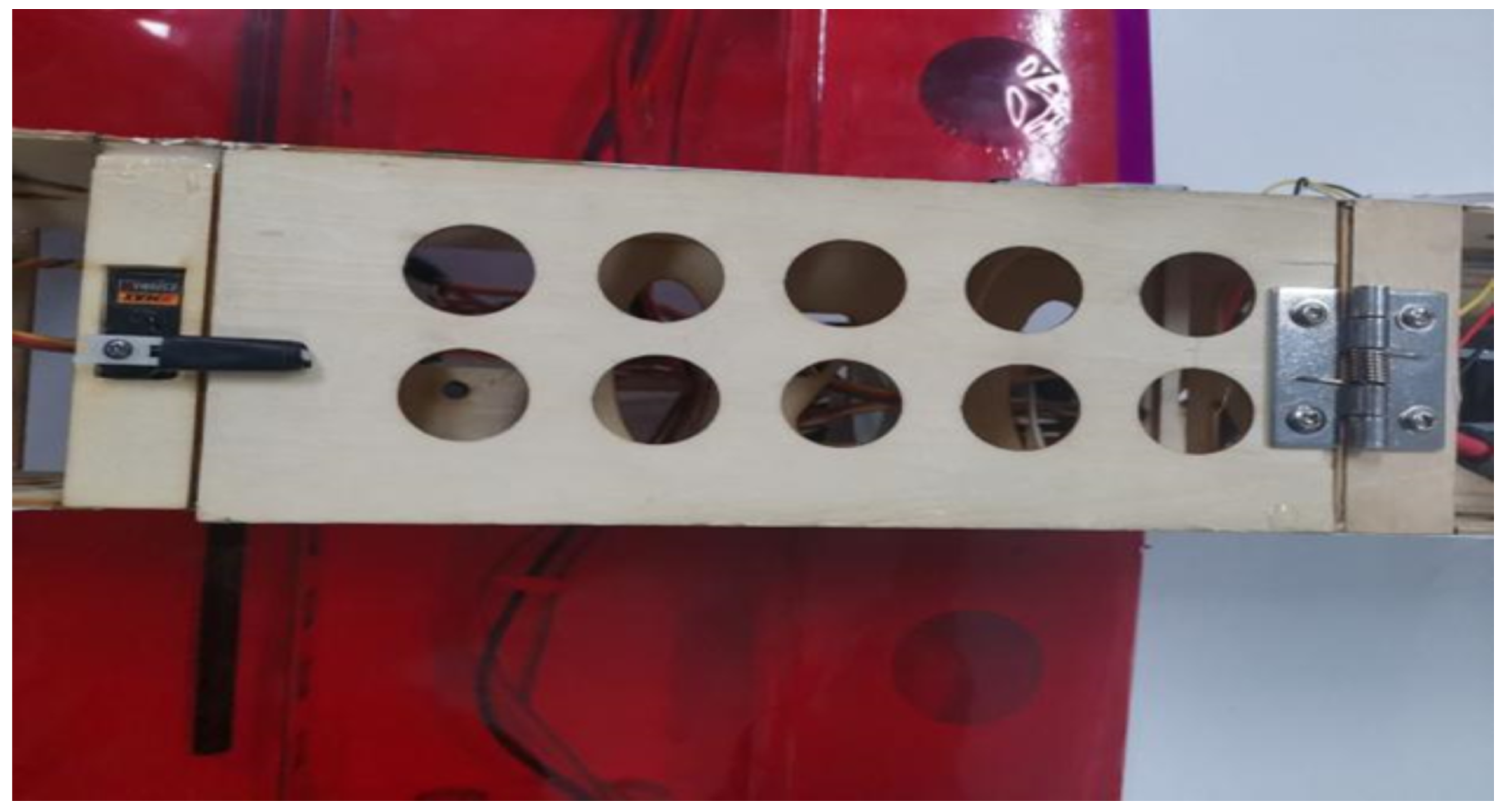
2.8.2. The Drone’s Throwing Mechanism

The UAV’s delivery mechanism, as shown in Figure 19, designed to be cost-effective and simple, uses a lever-arm release connected to the flight control system to drop a 500 mL water bottle without delay. Upon reaching the drop-off point, the flight controller commands the servo to rotate, opening the cargo bay door by the bottle’s weight. A spring hinge at the door prevents ground contact upon opening, ensuring it re-closes after delivery to avoid damage during landing.

3. Overview of Image Recognition Technology

3.1. Basic Composition of Image Recognition System

The image recognition system processes image data collected by the UAV, classifying, describing, and identifying targets or scenes to support UAV operations [56,57,58,59]. Figure 20 shows a series of images collected for this study.

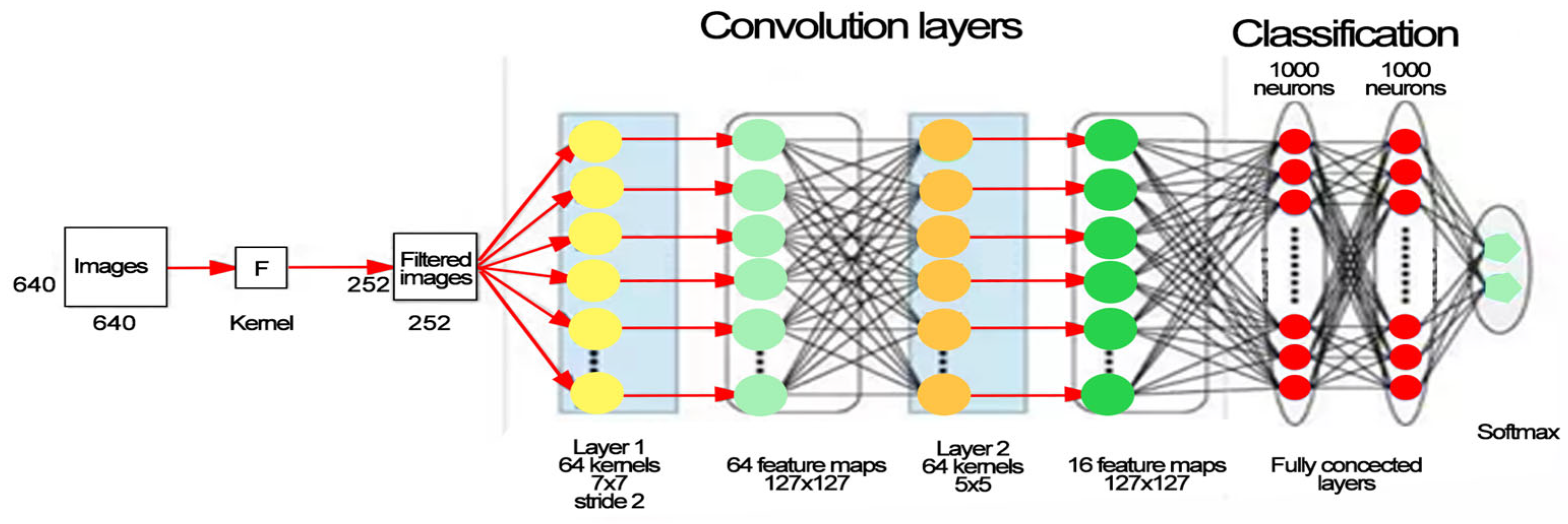
3.2. Image Recognition Algorithm and Implementation

In this study, experiments were conducted using two algorithms, OpenCV and the YO-LO deep-learning algorithm, as shown in Figure 21, for processing the same images for detection. The left figure shows an example of the OpenCV algorithmic detection, where the target is not accurately framed; the right figure demonstrates an example of the YOLO-based deep-learning algorithm, where the target is accurately framed. It is clear that in complex environments with a variety of distractions, conventional vision may not be able to completely filter out impurities to recognize a target. However, YOLO-based deep learning can accurately recognize targets in complex environments, showing high recognition accuracy and robustness. So, we chose YOLO-based deep learning as our target recognition algorithm.

The purpose of the image recognition system in this study is to automate and interpret the image recognition tasks for the delivery of fixed-wing UAVs, providing effective information support for the design and control of the UAVs. Figure 22 presents a schematic diagram of the image recognition system developed in this study.

Feature Extraction Algorithm

According to References [60,61], this study utilizes a feature extraction algorithm based on convolutional neural networks (CNNs) because they offer the following advantages:

CNNs can automatically learn and extract useful features from images without the need for manual design or selection;

Through multilayer convolutional structures, CNNs can extract different levels of features from images, ranging from low-level edges, lines, and colors to high-level objects, scenes, and semantics [62,63];

CNNs can map images directly to target categories through end-to-end training, without the need for additional feature encoding or classifiers.

The principle of CNNs involves using convolutional operations for the local receptive-field processing of images, thereby extracting local features. A convolutional operation acts as a filter, applying a weighted summation to a small area around each pixel point in the image to produce a new pixel value. The parameters of the convolutional operation are defined by the convolutional kernel, a matrix representing the weighting method for the area around each pixel point. The training process of CNNs, through backpropagation algorithms, continuously updates the parameters of the convolutional kernels, aiming to align the network’s output as closely as possible with the image’s actual labels, as shown in Figure 23, which illustrates the architecture of a CNN. The training process of CNNs can be seen as a feature-learning process, enabling convolutional kernels to automatically adapt to features within the image, thus extracting useful information [64,65].

3.3. Target Identification Applications

3.3.1. The Challenge and Demand of Target Identification

As shown in Figure 24, the UAV delivery task uses a UAV to simulate a logistic delivery scenario and accurately deliver simulated packages to ground targets. The mission is characterized as follows:

UAVs are required to complete reconnaissance and delivery tasks in an autonomous flight mode, without the use of any devices for real-time control or autonomous flights;

The flight speed and altitude of each UAV are restricted, necessitating quick target identification and localization within a short timeframe;

The target may be stationary or moving, and it may have various shapes, colors, and textures, potentially with obstructions and interference, requiring high recognition accuracy and robustness;

The UAV’s camera may be affected by lighting, noise, motion blur, etc., requiring image preprocessing and enhancement.

Given these characteristics, the target recognition system in this study needs to meet the following requirements:

Capable for detecting the target’s position and size in real-time video streams and outputting the target’s coordinates and framework;

Able to recognize the target’s category, outputting the target’s label and confidence level;

Adaptable to different targets and scenarios, with strong generalization capability and robustness;

Able to operate with limited computational resources and storage space, ensuring high efficiency and portability.

3.3.2. Target Recognition Scheme for UAV Dropping

To meet the requirements for target recognition, this study adopts the following approach: The study utilizes the YOLO series of deep-learning algorithms to train the target recognition model. The YOLO series includes various versions, such as YOLOv5n, YOLOv5s, YOLOv7, YOLOv8n, and YOLOv8s. This study sequentially employed these deep-learning algorithms to train the target recognition model and conducted model evaluations. As shown in Figure 25, the YOLOv8n model demonstrated superior recognition accuracy, recall rate, and recognition speed compared to the other models [66].

Table 8. Performance evaluation of each model in the YOLO series.

Model	Precision	Recall	[email protected]	S (m)
YOLOv5s	0.823	0.672	0.726	5.5
YOLOv5n	0.823	0.606	0.687	3.6
YOLOv7n	0.876	0.721	0.785	3.5
YOLOv8s	0.896	0.856	0.854	3.4
YOLOv8n	0.910	0.925	0.869	2.8
YOLOv8x	0.904	0.910	0.814	3.4
YOLOv8l	0.890	0.897	0.809	3.8

is performance evaluation of each model in the YOLO series.

This study initially collected target image data in various scenarios and periods [67]. Subsequently, the EasyData data-processing platform was utilized to categorize and label the original images, ultimately yielding 12,004 labeled images. To enhance the speed of the model training, a PyTorch environment was configured. Utilizing both a central processing unit (CPU) and a graphics processing unit (GPU) for simultaneous training in the YOLOv8 deep-learning framework, the model underwent 300 training cycles, resulting in the most performant model. The exported precision and recall curves after the training completion are depicted in Figure 25. Recall is the ratio of correctly detected targets to the total actual target count, with a higher recall rate signifying more accurate target detection [68,69]. From Figure 25, it can be deduced that the model developed in this study achieves a precision of 90% and a recall of 99.5%, indicating superior performance in target detection tasks. Through the model training described earlier, a highly accurate target recognition model was obtained, referred to in this study as the Open Neural Network Exchange (ONNX) target model. This model, based on deep learning, is capable for detecting and classifying targets within a single image [70]. By retrieving video streams from network cameras and employing OpenCV’s built-in cv2. readNet function, the ONNX target model developed in this study is used to perform inference on video streams, achieving effective target detection. Figure 26 illustrates the OpenCV target detection process.

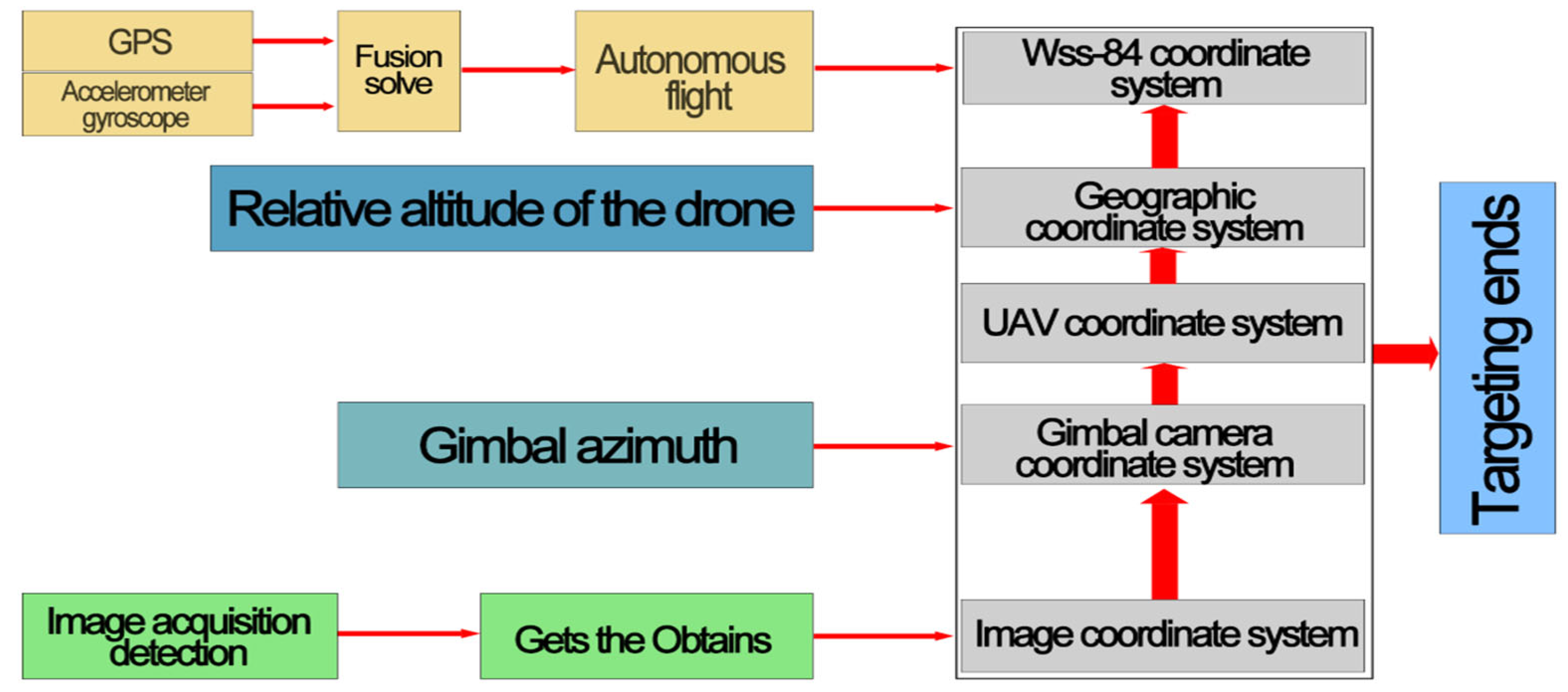
3.3.3. Target Coordinate Information Solution

To localize targets detected in video streams, it is essential to obtain parameters, such as latitude, longitude, altitude, and attitude angles, at the time of the UAV capture. These parameters can be acquired from the UAV’s telemetry data. Utilizing the UAV’s attitude angles, actual ground coordinates are transformed via rotation and translation into a local coordinate system with the UAV as the reference point, such as Figure 27.

Through prior work, we can accurately identify and frame targets within the original image, leading to the critical next step for computing target coordinate information [71]. Target coordinate computation has broad applications in computer vision and image processing, allowing for the precise localization and tracking of targets in the three-dimensional world. For instance, in autonomous driving, robotic navigation, and UAV flights, target coordinate computation aids in determining the position and orientation of vehicles, robots, or UAVs on the ground or in the air, facilitating flights and path planning. Accurate target coordinates relative to the UAV are necessary for simulating deliveries, such as dropping a 500 mL water bottle as a payload.

With Zhang Dingyou’s method being adopted in this study [72] during the camera calibration, capturing chessboard patterns at different angles and distances helps to obtain the camera’s internal parameters and distortion coefficients. Selecting the best set of distortion coefficients reduces calibration errors for distortion correction. Having obtained the camera’s intrinsic and extrinsic parameters—K as the camera’s intrinsic matrix and $\left[R|T\right]$ as the rotation and translation matrix—precise target identification allows us to determine the target center’s pixel coordinates, $\left(u, v\right)$. The following equations normalize pixel coordinates to planar coordinates, $\left(x, y\right)$:

$$\begin{gathered} x=u/f \\ y=v/f \end{gathered}$$

(20)

The inverse matrix, $K^{-1}$, of the normalized planar coordinates, $\left(x,y\right)$, and the inverse matrix of the camera’s internal parameter matrix can be used to convert the normalized coordinates into coordinates in the camera’s coordinate system, $\left(x\_c,y\_c,z\_c,1\right)$ as follows:

$${\left.[x_{-}{c}_{,}{y}_{-}c,1\right]}^{\mathrm{T}}=K^{-1}\times [x,y,1{]}^{\mathrm{T}}$$

(21)

The coordinates in the camera’s coordinate system, $\left(x\_c,y\_c,z\_c,1\right)$, are then rotated by the rotation matrix (R) and translation vector (T) from the out-of-camera parameters to coordinates $\left(x,y,z\right)$ in the real-world coordinate system as follows:

$${[X,Y,Z,1]}^T={[R\mid T]}^{-1}\times {\left[x_{-}c,y_{-}c,z_{-}c,1\right]}^T$$

(22)

Using the above process, the image coordinates, (u, v), can be converted into real-world coordinates, $\left(X, Y, Z\right)$, which, in this study, also need to be converted into coordinates in WGS84. In this study, let A be the radius of the unit circle and E be the first eccentricity of the Earth. Let the equatorial radius of the reference ellipsoidal sphere be c, the polar radius of the reference ellipsoidal sphere’s bed, and let B be the latitude of the UAV, and the formulae are as follows:

$$\left\{\begin{array}{l}{A}^2=\frac{a^2-b^2}{a^2}\\ N=\frac{a}{\sqrt{1-A^2}\mathrm{s}\mathrm{i}{\mathrm{n}}^{2}B}\end{array}\right.$$

(23)

Finally, the latitudinal and longitudinal information of the target in WGS84 is determined using the following equations:

$$\left\{\begin{array}{l}L=\arctan \frac{Y}{X}\\ M=\arctan \frac{Z+A\times E^2\sin B}{\sqrt{X^2+Y^2}}\\ H=\frac{\sqrt{X^2+Y^2}}{\cos B}-A\end{array}\right.$$

(24)

where L is the longitude of the target, M is the dimension of the target, and H is the altitude of the target (0 for ground targets). So far in this study, the coordinate information of the target has been obtained.

3.3.4. Target’s Throwing Test

When the target is detected, the vertical projection distance of the target relative to the UAV is obtained, and the UAV starts to adjust its attitude to be colinear with the target. Then, the onboard computer releases the dropping command to control the switch of the dropping bin so that the 500 mL water bottle makes a free-fall motion to hit the target. In this study, we set the distance of the target from the vertical ground projection of the UAV as S, the height of the UAV drop as U, the cruising speed of the UAV as V, and X is the distance between the drop’s ground-landing point and the target. The formulae are as follows:

$$\left\{\begin{array}{c}U=\frac{1}{2}g{t}^2\\ S=Vt\end{array}\right.$$

(25)

where g is the acceleration of gravity, and t is the falling time. To find the best throwing height and cruising speed, this study carried out a throwing test many times because the positioning error of the GPS is around 5 m. It also takes into account the wind resistance and the wind direction influences to ensure the smooth flight of the UAV. Thus, this study limits the throwing height to 8–12 m, and the speed is limited to 11–12 m/s. The test results are shown in

Table 9. Test data of multiple throwing experiments.

Frequency	Height	Speeds	Drop Distances	Landing Errors
1	8 m	11 m/s; 12 m/s	13.91 m; 15.18 m	4.12 m; 4.32 m
2	8.5 m	11 m/s; 12 m/s	14.34 m; 15.65 m	4.13 m; 4.42 m
3	9 m	11 m/s; 12 m/s	14.76 m; 16.10 m	4.03 m; 4.11 m
4	9.5 m	11 m/s; 12 m/s	15.16 m; 16.54 m	3.98 m; 3.60 m
5	10 m	11 m/s; 12 m/s	15.55 m; 16.67 m	2.86 m; 2.66 m
6	10.5 m	11 m/s; 12 m/s	15.94 m; 17.39 m	2.86 m; 2.65 m
7	11 m	11 m/s; 12 m/s	16.31 m; 17.80 m	2.99 m; 3.01 m
8	11.5 m	11 m/s; 12 m/s	16.68 m; 18.02 m	2.86 m; 3.05 m
9	12 m	11 m/s; 12 m/s	17.04 m; 18.15 m	3.08 m; 3.12 m
10	12 m	11 m/s; 12 m/s	13.5 m; 12 8 m	4.95 m; 5.18 m

. In Table 9, frequencies 1–9 indicate that we conducted nine rounds of experiments, and in each round, dozens of experiments were carried out at speeds of 11 m/s and 12 m/s. The simple random sampling method was adopted to extract five pieces of data and calculate the average value. Two sets of data, including the delivery distance and landing error, were obtained for each round, corresponding to speeds of 11 m/s and 12 m/s, respectively.

As shown in Figure 28, when the UAV’s throwing height is 10 m, the error in the target point is 2.66 m when throwing/dropping the 500 mL water bottle at 12 m/s. Figure 28 shows the simulated drop point of the 500 mL water bottle; we can see that when the UAV’s throwing height is 10 m, the drop point falls within the effective throwing range of 3 m when throwing/dropping the 500 mL bottle of water at 12 m/s. The requirement of this study is thus satisfied. In Figure 28, we can see that most of the landing points reach a relatively accurate distance, but there are still some landing points beyond the effective range of 5 m, which is mainly affected by the weather; the wind is too strong, and the landing point is offset, but compared with the overall landing point, such similar errors can be ignored. According to the analysis of nearly one hundred kinds of data from our previous nine rounds of experiments, we established a multiple linear regression model for the analysis, and the multiple linear regression model is as follows:

$$e_i={\beta }_0+{\beta }_1{h}_i+{\beta }_2{s}_i+{ϵ}_i$$

(26)

where $h_i$ represents the throwing height (height) of the ith experiment; $s_i$ represents the throwing speed (speed) of the ith experiment; $e_i$ represents the corresponding landing error; ${\beta }_0$ is the intercept of the model and represents the baseline value of the landing error when both the height and speed are zero; ${\beta }_1$ represents the coefficient of the height, which represents the expected amount of change in the landing error for each unit of change in the height; ${\beta }_2$ represents the coefficient of the velocity, which represents the expected amount of change in the drop point error for each unit of change in the velocity; and ${\epsilon }_i$ represents the error term, which represents the random error that the model fails to account for. The requirements of this study are met, as the drop point falls within the effective drop range of 3 m when throwing/throwing the 500 mL bottle at a UAV drop height of 10 m. The water velocity is 12 m/s, and the error term is minimized.

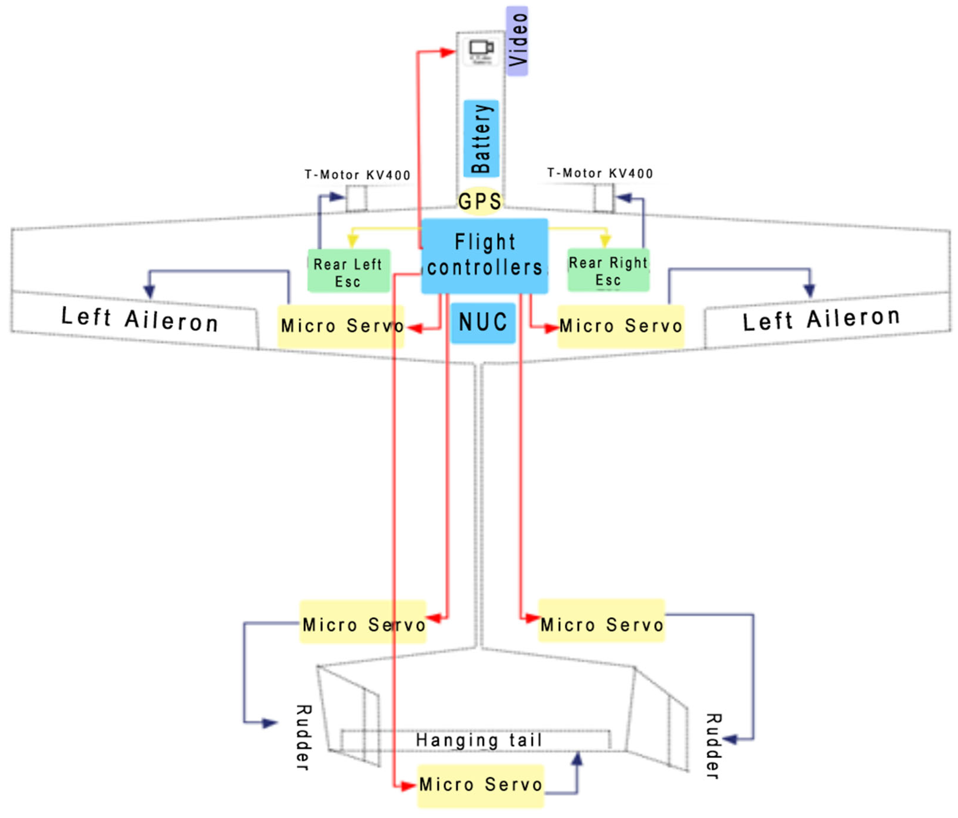
4. Flight Control System

4.1. Flight Control System Overview

At the center of the system, as shown in the Figure 29, is the flight controller, which is connected to the battery and GPS. The battery provides power, and the GPS module is used for positioning and navigation. The flight controller controls several parts of the UAV, including the left and right ailerons, the rudder, and the hanging tail, through several micro-servo motors. These servomotors are responsible for adjusting the position of the respective components to change the direction of the flight and attitude of the UAV. Two electronic speed controllers (ESCs) are connected to the rear left and rear right motors. The ESCs control the speed of the motors, which, in turn, control the thrust and flight speed of the UAV. An NUC is connected to the flight controller for processing more complex data or performing advanced flight tasks. An image recognition module is also connected to the battery.

4.2. Fundamentals of Control Law Design and Optimization

Previously, we established the dynamic equations of the aircraft. In light of this, this study employs a robust advanced control law to enable the autonomous flight, stability, and maneuvering of UAVs. The objective of this control law is to minimize the quadratic performance index while ensuring system stability and compliance with constraints. Additionally, it can address system uncertainties and disturbances, thereby enhancing the control law’s robustness and adaptability.

Assuming that the UAV’s dynamic model can be described by a linear time-invariant state–space model, the control objective is to enable the UAV to engage in autonomous flights along a predetermined route while meeting specific performance indices and constraints. Utilizing a robust control law, the feedback gain provided by the linear–quadratic regulator (LQR) serves as the initial value for the model predictive control (MPC). Furthermore, by leveraging the MPC’s predictive capabilities and constraints, the performance and robustness of the control law are enhanced.

Extensive simulation experiments and field tests have been conducted to fine-tune the parameters of the control law to adapt to various complex environments. The optimization outcomes indicate that the control law enables the UAV to fly along the preset course, satisfying certain performance indices and constraints. Furthermore, the control law can manage system uncertainties and disturbances, improving its robustness and adaptability. The comparative results of this control law against other control laws are depicted in

Table 10. Comparison between the optimized control rate and the traditional control rate.

Command	Value	New Value
INS_GYR1_CAL	39.49276	17.75362
INS_GYR2_CAL	22.48535	12.24728
INS_GYR20FFS_X	0.02180705	−0.002505591
INS_GYR20FFS_Y	−0.007266462	−0.008429104
INS_GYR20FFS_Z	0.007931517	0.006754024
INS_GYR3_CAL	37.83039	25.74678
INS_GYR30FFS_X	0.007584155	−0.003129626
INS_GYR30FFS_Y	−0.03437863	−0.02893007
INS_GYR30FFS_Z	0.01442171	0.01368616
INS_GYR0FFS_X	0.002235635	0.006046154
INS_GYR0FFS_Y	0.005703443	0.01224557
INS_GYR0FFS_Z	−0.01396238	−0.01341222
STAT_BOOTCNT	163	161
STAT_RUNTIME	67,684	62,540
TECS_PITCH_MAX	20	15
TKOFF_THR_DELAY	2	0
TKOFF_THR_MT	15	0
TKOFF_THR_MT	1	0

.

4.3. Implementation and Verification of the Control Algorithm

The control algorithm is divided into three primary layers: control, stabilization, and maneuvering. The control layer plans the UAV’s trajectory and desired posture based on mission requirements and GPS data [73]. The stabilization layer calculates the UAV’s attitude error and desired angular velocity, leveraging the expected posture and sensor data. The maneuvering layer computes the UAV’s control inputs from the expected angular velocity and sensor data, outputting them to the actuators.

The control algorithm is predominantly written in C and operates on the STM32F103 microcontroller. This research employs Keil µVision5 as the development environment, FreeRTOS as the real-time operating system, and the HAL library for hardware abstraction.

Hardware-in-the-loop simulations (HILSs) and field flight testing are employed for the evaluations. HILS is a methodology that connects actual hardware with computer simulation models, allowing for effective control-algorithm testing and debugging without the necessity of flights [74]. This research utilizes MATLAB/Simulink as the simulation platform and X-Plane for the flight dynamics model, with serial and UDP communications facilitating data transmission, thus implementing the UAV’s HILS system. Field flight tests serve to ultimately validate the control algorithm, assessing its performance and robustness in real-world settings. Multiple flight trials have confirmed the UAV’s capabilities for autonomous flight, stability, and maneuvering, as well as the completion of reconnaissance, identification, and strike missions.

5. Test Process and Result Analysis

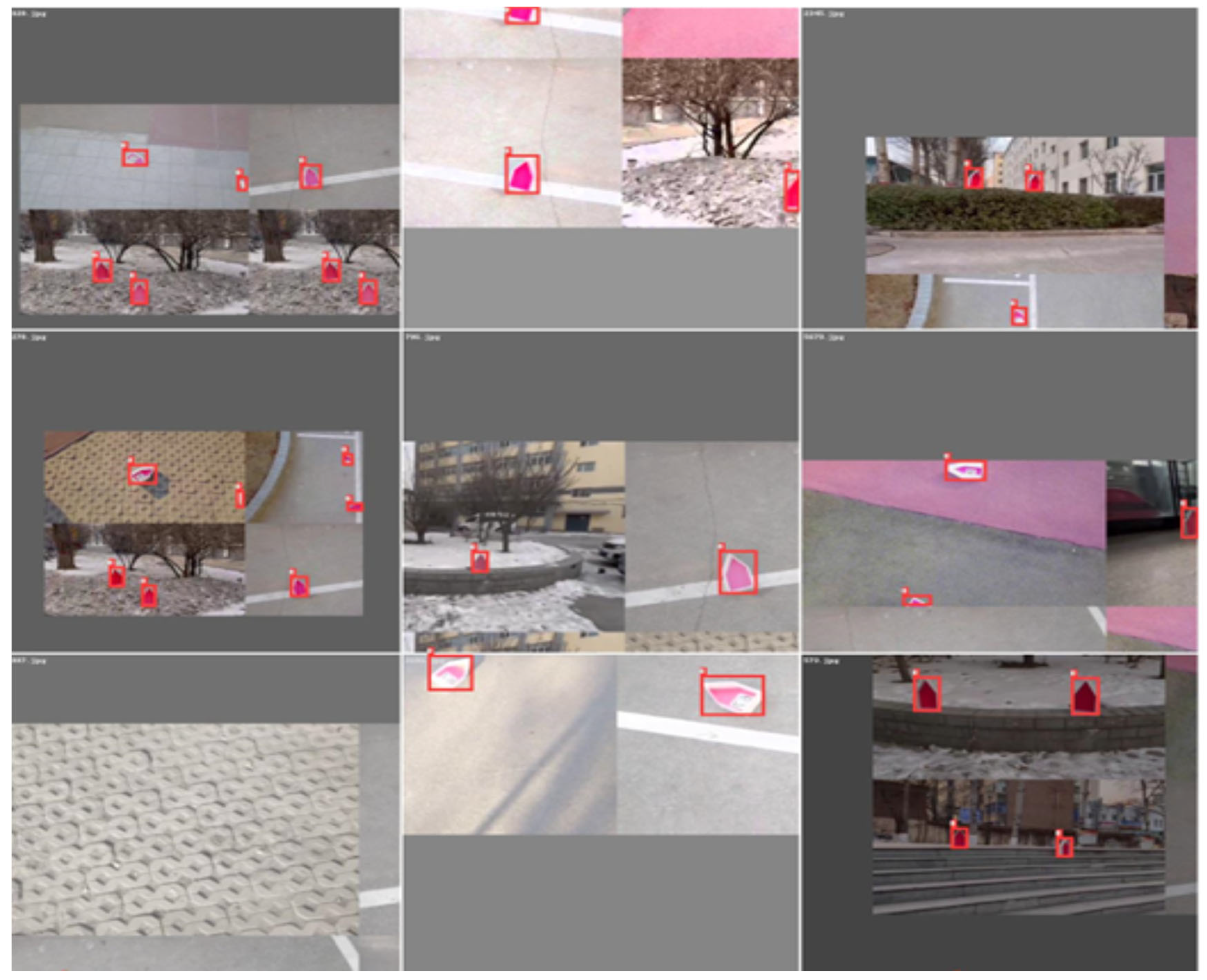
5.1. Image Recognition Effect Test

To validate the performance and effectiveness of the target recognition system in this study, we purchased unopened 500 mL bottles of water that met the national standard to be used as simulated small packages. In an open field, different targets, both stationary and moving, with different shapes, colors, and textures, as well as some occlusions and interferences, were set up as strike targets for the UAV [75]. The model aircraft was allowed to reconnoiter, identify, and strike the targets in an autonomous flight state, and the flight trajectories of the UAV, the results of the image recognition, the angles and times of the throws, and the effects of the strikes were recorded. The results of the image recognition are shown in Figure 30, and the flight path planning of the UAV is shown in Figure 31.

5.2. Field Experiments Compared to Those of Other Ultra-Low-Cost Drones

5.2.1. Test Environment and Conditions

In outdoor experiments, flights were performed using small fixed-wing unmanned aerial vehicles (UAVs) available on the market within the price range of USD150–200, as well as a hand-launched fixed-wing UAV optimized to a cost of approximately USD100. To minimize the variables, all the flights were conducted under clear, windless weather conditions at low altitudes. The flight plans and waypoint diagrams were designed for a flight area of 220 by 50 m, with the flight altitudes ranging from 10 to 60 m and at a speed of 20 m/s. The waypoint diagrams for each UAV were developed accordingly. Figure 32 shows a map of the waypoints of the drones on the market. Figure 33 is UAV waypoint diagram optimized in this study.

The commercially purchased UAV has a flight time of 1 min and 6 s, while the UAV in this study has a flight time of 1 min and 32 s. Relevant flight videos are shown in Videos S1 and S2. Their respective advantages and disadvantages in various aspects are analyzed in detail in Section 5.2.2. The test conditions were as follows:

• Information on the takeoff point, waypoint, landing point, and target point of the unmanned aerial vehicle, as well as flight parameters and control parameters, appear on the flight control panel. It is prohibited to use any equipment for the real-time control and autonomous flight of the model;
• The drone carried a simulated package consisting of an unopened 500 mL bottle of water;
• The drone’s mission simulated the precise delivery of a courier package by a low-cost drone, with the model aircraft in the autonomous flight mode, while completing parcel organizer identification and parcel-dropping tasks;
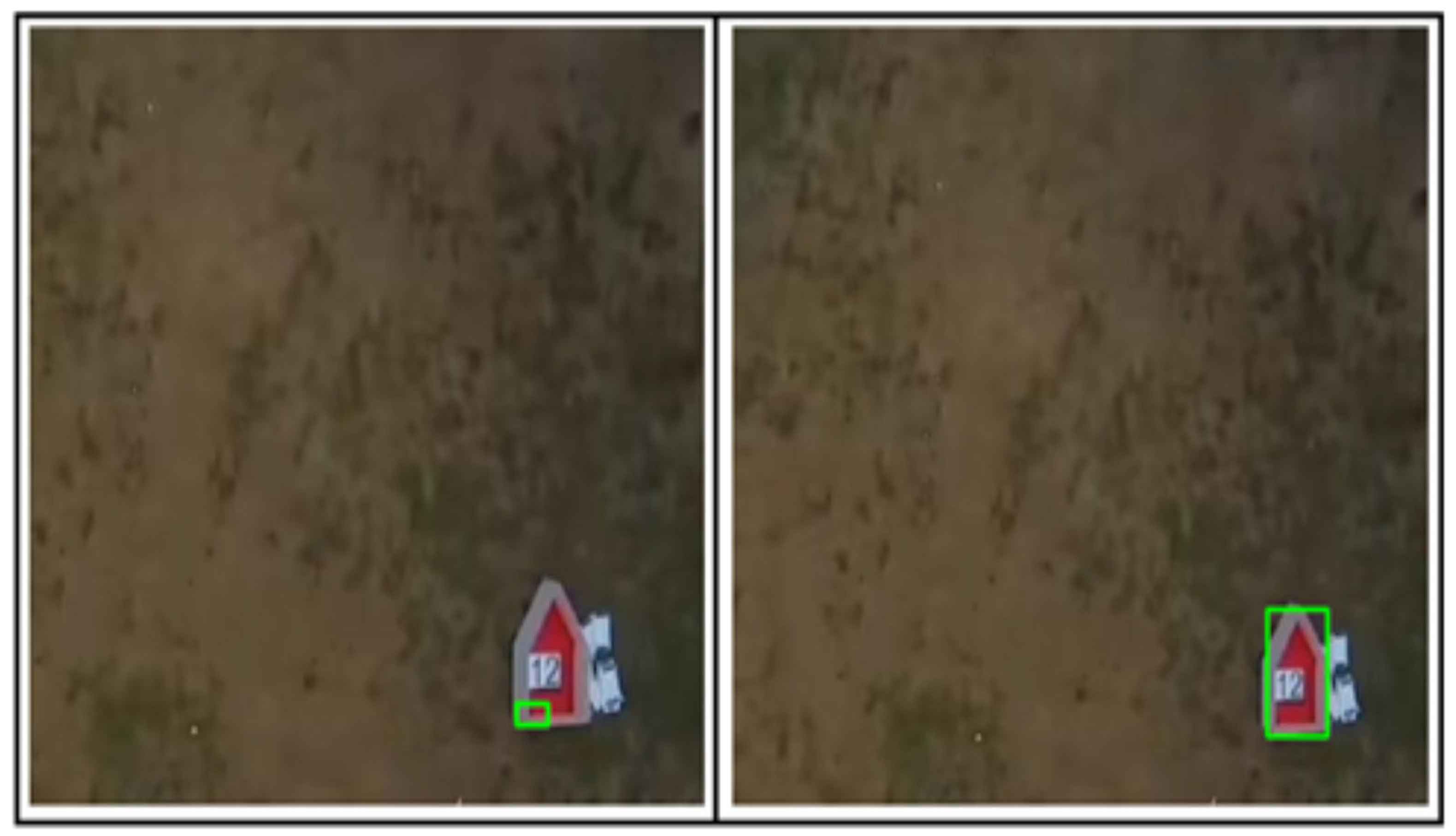
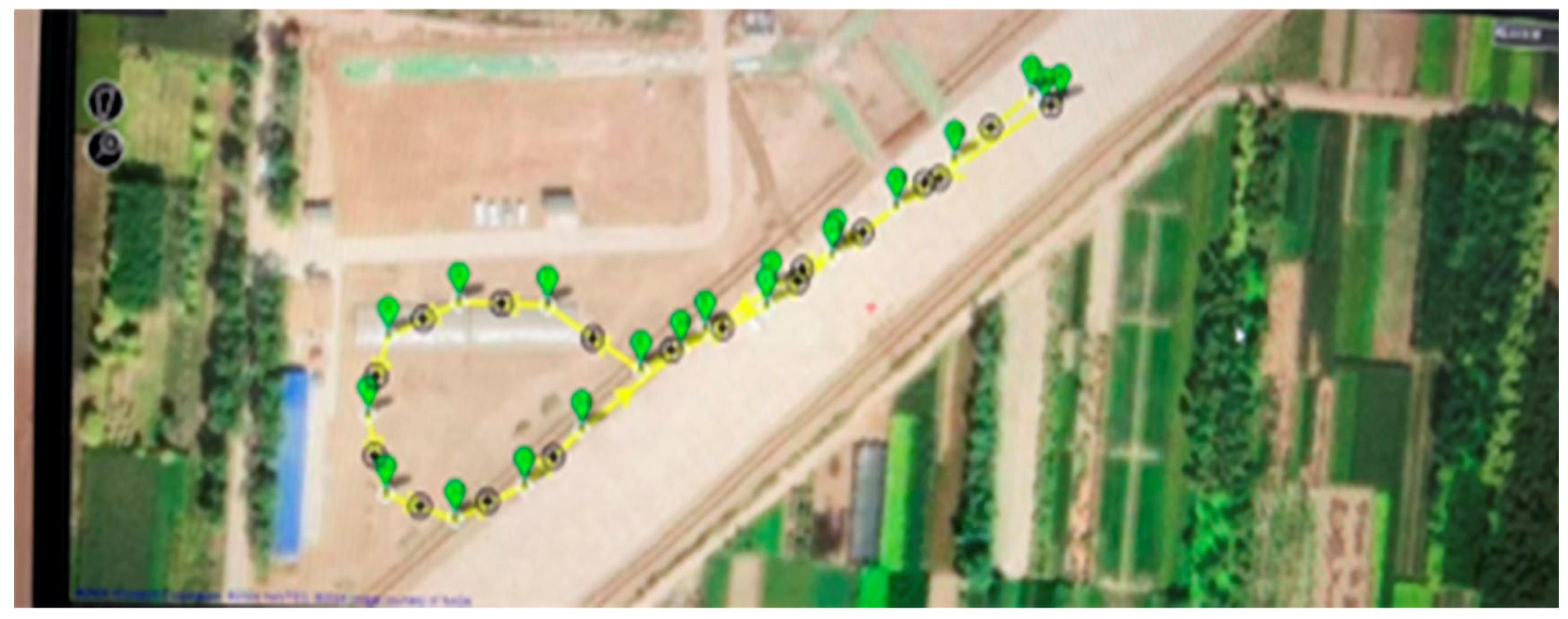
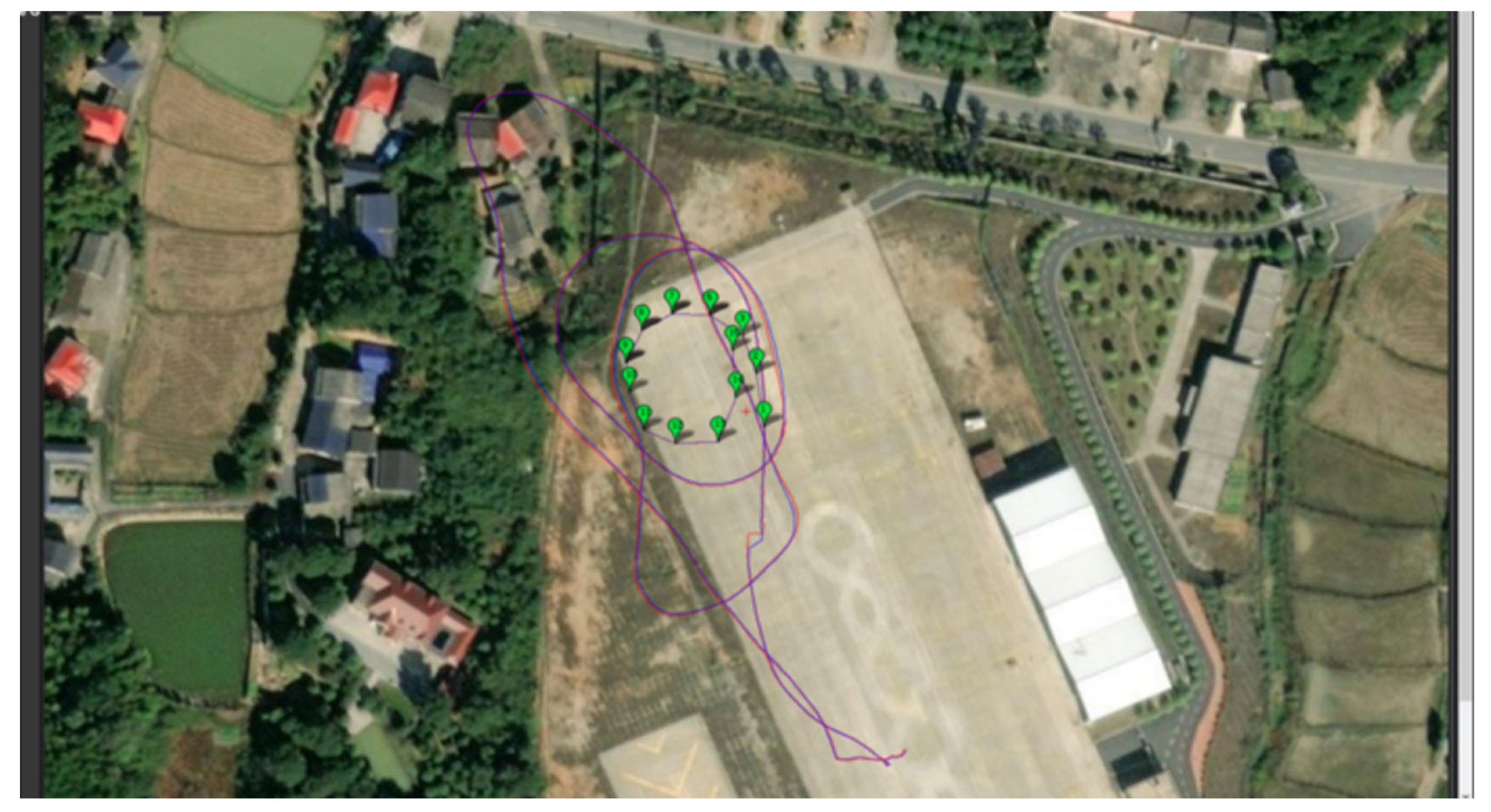
• The flight process and results of the UAV were recorded and displayed on a computer at the ground station, including data on the UAV’s position, speed, attitude, control inputs, and image information, as well as images of the UAV’s flight trajectory, the location of the parcel organizer, and the point at which the parcel was released.

5.2.2. Presentation and Analysis of Test Results

We conducted several test experiments, and the process of each experiment is as follows.

The UAV carries a simulated parcel and automatically enters autonomous flight mode after launching, following a predetermined flight path. During the flight, a computer at the ground station is used to monitor and record real-time data, such as the UAV’s position, velocity, attitude, control inputs, and flight path images. Autonomous flight algorithms and control laws enabled the UAV to fly stably along the preset route, meeting specific performance indicators and constraints and demonstrating the effectiveness and superiority of the autonomous flight and control systems.

When approaching the target, the UAV automatically switched to reconnaissance mode, using an image recognition system to search for and locate the target. Despite the complex background and lighting conditions, the image recognition system was able to identify the target quickly and accurately, demonstrating its accuracy and reliability.

After successfully identifying the target, the UAV begins to drop, utilizing the control system to accurately drop the simulated package. The control system dynamically adjusts the control inputs according to the position and motion of the target, enabling the UAV to release the simulated parcel at the optimal time and position, thus highlighting the flexibility and robustness of the control system.

After the release of the simulated package, the UAV automatically resumed its autonomous flight mode and returned to the landing site along the predetermined route, thus completing the mission. After the mission was completed, the fixed-wing aircraft described in this paper was flown against a common aircraft available on the market under the same flight conditions. After exporting the flight logs for this paper, using the mission planner, the roll, pitch, and yaw data were presented from the logs in 40 mm units and plotted separately using the origin. The final results were compared with those of commercially available airplanes to obtain Figure 34.

The test results of this study are shown in Figure 34.

As illustrated, a comparison of the angles before and after the optimization reveals that the UAV optimized in this study exhibits a smaller deviation from the expected values while also meeting specific performance indices and constraints. This indicates the superior control performance and structural design of this UAV, highlighting the effectiveness and superiority of the autonomous flight algorithms and control laws that were implemented. Moreover, the UAV successfully conducts target search and location, demonstrating the accuracy and reliability of the image recognition system. Following the precise target strike and smooth return to the base, the comprehensive and practical nature of the UAV design and control scheme proposed in this study are further verified.

6. Conclusions and Prospects

In this study, a development path is described for a DIY ultra-low-cost fixed-wing UAV for delivery missions. An advanced flight control system, based on LQR and MPC, was designed and implemented. Using sensors and actuators on the flight control board, the UAV is able to fly, stabilize, and operate autonomously, taking into account system uncertainties and disturbances. The parameters and algorithms of the flight control system are optimized by adjusting parameters, such as the weight matrix, prediction window, sampling time, and covariance matrix. The creation and implementation of a deep-learning-based image recognition system, utilizing the YOLOv8 algorithm and coordinate transformation technology, are outlined. The effectiveness and superiority of this UAV system are verified through simulation experiments and flight tests, which demonstrate the system’s ability to accomplish target transportation and delivery. This system satisfies specific performance metrics and constraints with high accuracy, flexibility, stability, robustness, and utility. Each of these components is integrated into a cohesive system, making it unmatched by traditional methods in last-mile delivery applications. According to the test results, this paper draws the following conclusions:

• The total production cost of the UAV described in this paper is 101 USD, while the generation cost of the same type of UAV on the market is 280 USD, which greatly reduces the production cost and usage cost;
• We designed a streamlined wing and dual vertical h-shaped tail, based on an accurate aerodynamic analysis, which has higher lift, strength, and stiffness and lower drag and lateral drag than the same type of aircrafts, in which our wing model parameterization meets the requirements and the results converge. The displacement reduces the fuselage oscillations, and the volume factor is reduced by 10% to 20%, which shows that the aircraft has a more optimized performance compared to the same type of commercially available aircrafts;
• We designed an autonomous projectile mechanism and spring hinges, which are more flexible and protect the projected package compared to marketed UAVs;
• After several test experiments, we found that the UAV optimized in this study has less deviation from the desired values and meets specific performance metrics and constraints. This demonstrates the superior control performance and structural design of the proposed UAV, highlighting the effectiveness and superiority of the autonomous flight algorithms and the implemented control laws. In addition, the UAV successfully performed target search and localization, demonstrating the accuracy and reliability of the image recognition system. Based on the precise target strike and smooth return to the base, the comprehensiveness and practicality of the UAV’s design and control schemes proposed in this study are further verified.

In future work, we can further improve the accuracy and robustness of the autonomous flight algorithm, as well as the scalability and compatibility of the flight control system, to enhance the flight function.

References

1. Goran, P.; Sasa, S.; Marina, I.-K. Application of Ray Cast Method for Person Geolocalization and Distance Determination Using UAV Images in Real-World Land Search and Rescue Scenarios. Expert Syst. Appl. 2024, 237, 121495. [Google Scholar]
2. Yi, Z.; Hongda, Y. Application of Hybrid Swarming Algorithm on a UAV Regional Logistics Distribution. Biomimetics 2023, 8, 96. [Google Scholar] [CrossRef] [PubMed]
3. Peck, M. Close encounters of the drone kind. Aerosp. America 2015, 53, 18–23. [Google Scholar]
4. Cui, L.; Zhou, Q.; Huang, D.; Yang, H. Fixed-Time Disturbance Observer-Based Fixed-Time Path Following Control for Small Fixed-Wing UAVs under Wind Disturbances. Int. J. Adapt. Control Signal Process. 2023, 38, 23–38. [Google Scholar] [CrossRef]
5. Popova, I.; Abdullina, E.; Danilov, I.; Marusin, A.; Marusin, A.; Ruchkina, I.; Shemyakin, A. Application of the RFID technology in logistics. Transp. Res. Procedia 2021, 57, 452–462. [Google Scholar] [CrossRef]
6. Deng, M.; Yang, Q.; Peng, Y. A Real-Time Path Planning Method for Urban Low-Altitude Logistics UAVs. Sensors 2023, 23, 7472. [Google Scholar] [CrossRef] [PubMed]
7. Zhang, W.; Jia, W.; Ma, Y.; Yan, X.; Liu, Y.; Song, G.; Yang, X. A Password-Sending-And-Receiving Device for Unmanned Aerial Vehicle for Logistics Delivery and Distribution. U.S. Patent Application No. 16/300,563, 30 May 2019. [Google Scholar]
8. Ko, Y.D. The airfare pricing and seat allocation problem in full-service carriers and subsidiary low-cost carriers. J. Air Transp. Manag. 2019, 75, 92–105. [Google Scholar] [CrossRef]
9. Inghels, M.; Mee, P.; Diallo, O.H.; Cissé, M.; Nelson, D.; Tanser, F.; Asghar, Z.; Koita, Y.; Laborde-Balen, G.; Breton, G. Improving Early Infant Diagnosis for HIV-Exposed Infants Using Unmanned Aerial Vehicles for Blood Sample Transportation in Conakry, Guinea: A Comparative Cost-Effectiveness Analysis. BMJ Glob. Health 2023, 8, e012522. [Google Scholar] [CrossRef] [PubMed]
10. Yang, W.; Shi, Z.; Zhong, Y. Robust Adaptive Three-Dimensional Trajectory Tracking Control Scheme Design for Small Fixed-Wing UAVs. ISA Trans. 2023, 141, 377–391. [Google Scholar] [CrossRef]
11. Santos, N.P.; Lobo, V.; Bernardino, A. Fixed-Wing Unmanned Aerial Vehicle 3D-Model-Based Tracking for Autonomous Landing. Drones 2023, 7, 243. [Google Scholar] [CrossRef]
12. Alwaseela, A.; Wheeler, T.A.; Dever, J.; Lin, Z.; Arce, J.; Guo, W. Assessing Fusarium Oxysporum Disease Severity in Cotton Using Unmanned Aerial System Images and a Hybrid Domain Adaptation Deep Learning Time Series. Model. Biosyst. Eng. 2024, 237, 220–231. [Google Scholar]
13. Cheonghwa, L.; Hwanhee, K.; Baeksuk, C. Airdrop Operation and Autonomous Flight-Back Experiment of Dual Unmanned Aircraft. J. Inst. Control Robot. Syst. 2019, 25, 519–525. [Google Scholar]
14. Tong, Z.; Guo, J.; Wu, Q.; Xu, C. An Unmanned Aerial Vehicle Identification and Tracking System Based on Weakly Supervised Semantic Segmentation Technology. Phys. Commun. 2022, 54, 101758. [Google Scholar]
15. Fanghao, H.; Chen, X.; Xu, Y.; Yang, X.; Chen, Z. Immersive Virtual Simulation System Design for the Guidance, Navigation, and Control of Unmanned Surface Vehicles. Ocean Eng. 2023, 281, 114884. [Google Scholar]
16. Shakhatreh, H.; Sawalmeh, A.; Alenezi, A.H.; Abdel-Razeq, S. Mobile-IRS Assisted Next Generation UAV Communication Networks. Comput. Commun. 2024, 215, 51–61. [Google Scholar] [CrossRef]
17. Bokhtier, G.M.; Crawford, S.W.; Shahroudi, K.E. Integrated Systems Architectural Modeling with Architectural Trade Study of a UAV Surface-less Flight Control Systems for Wildfire Detection and Communication Utilizing MBSAP. INCOSE Int. Symp. 2023, 33, 229–250. [Google Scholar] [CrossRef]
18. Kuhara, S. Method of Displaying Flight Route of Unmanned Aerial Vehicle That Flies Autonomously, Terminal, and Non-Transitory Computer-Readable Recording Medium Storing Program. U.S. Patent 10,685,573, 16 June 2020. [Google Scholar]
19. Shalyhin, A.; Nerubatsky, V.; Denysova, S. The UAV Flight Route Optimization by Taking into Consideration the Wind Influence. Наука і Техніка Пoвітряних Сил Збрoйних Сил України 2018, 3, 20–24. [Google Scholar] [CrossRef]
20. Anosri, S.; Panagant, N.; Champasak, P.; Bureerat, S.; Thipyopas, C.; Kumar, S.; Pholdee, N.; Yıldız, B.S.; Yildiz, A.R. A Comparative Study of State-of-the-Art Metaheuristics for Solving Many-Objective Optimization Problems of Fixed Wing Unmanned Aerial Vehicle Conceptual Design. Arch. Comput. Methods Eng. 2023, 30, 3657–3671. [Google Scholar] [CrossRef]
21. Nikolas, H.; Christoph, B.; Michael, A. Performance Evaluation of Image-based Location Recognition Approaches Based on Large-scale UAV Imagery. In Proceedings of the Electro-Optical Remote Sensing, Photonic Technologies, and Applications VIII; and Military Applications in Hyperspectral Imaging and High Spatial Resolution Sensing II, Amsterdam, The Netherlands, 22–25 September 2014; Volume 9250, pp. 154–159. [Google Scholar]
22. Hassan, S.A. Effective Range of Unmanned Aerial Vehicle (UAV) in the Malaysian Army Tactical Operations. Appl. Mech. Mater. 2014, 3446, 399–403. [Google Scholar] [CrossRef]
23. Muzzi, F.A.G.; de Mello Cardoso, P.R.; Pigatto, D.F.; Branco, K.R.L.J.C. Using Botnets to Provide Security for Safety-Critical Embedded Systems—A Case Study Focused on UAVs. J. Phys. Conf. Ser. 2015, 633, 012053. [Google Scholar] [CrossRef]
24. Thomas, P.; Delbecq, S.; Pommier-Budinger, V.; Bénard, E. Modeling and Design Optimization of an Electric Environmental Control System for Commercial Passenger Aircraft. Aerospace 2023, 10, 260. [Google Scholar] [CrossRef]
25. Li, W.; Yang, Z.; Liu, K.; Wang, W. MIMO Multi-Frequency Active Vibration Control for Aircraft Panel Structure Using Piezoelectric Actuators. Int. J. Struct. Stab. Dyn. 2023, 23, 2350157. [Google Scholar] [CrossRef]
26. Lim, Y.X. Cognitive Human-Machine Interfaces and Interactions for Avionics Systems. Ph.D. Thesis, RMIT University, Melbourne, VIC, Australia, 2020. Available online: https://researchrepository.rmit.edu.au/esploro/outputs/doctoral/Cognitive-human-machine-interfaces-and-interactions-for-avionics-systems/9921957511601341 (accessed on 30 March 2024).
27. Pavithran, R.; Lalith, V.; Naveen, C.; Sabari, S.P.; Kumar, M.A.; Hariprasad, V. A Prototype of Fixed Wing UAV for Delivery of Medical Supplies. IOP Conf. Ser. Mater. Sci. Eng. 2020, 995, 012015. [Google Scholar] [CrossRef]
28. Sabri, F.; Elzaabalawy, A.; Meguid, S.A. Aeroelastic Behavior of a Flexible Morphing Wing Design for Unmanned Aerial Vehicle. Acta Mech. 2022, 233, 851–867. [Google Scholar] [CrossRef]
29. Liu, W.; Li, X.; Shen, Z.; Ma, C. A Digital Twin Method for Civil Aircraft Power Distribution System Based on Unity3D and Simulink. J. Phys. Conf. Ser. 2023, 2615, 012017. [Google Scholar] [CrossRef]
30. Zhou, Q.; Wei, Y.; Zhu, L. Research on Reliability Modeling of Unmanned Aircraft System Avionics Systems Based on 5G. Int. J. Distrib. Sens. Netw. 2019, 15, 1550147719860381. [Google Scholar] [CrossRef]
31. Sikorsky Aircraft Corporation. Aircraft Route Systems” in Patent Application Approval Process. Def. Aerosp. Week 2019, 103. [Google Scholar]
32. Madika, B.; Syahrial, A.Z. Study of Aluminum/Kevlar Fiber Composite Laminate with and without TiC Nanoparticle Impregnation and Aluminum/Carbon Fiber Composite Laminate for Anti-Ballistic Materials. Int. J. Light. Mater. Manuf. 2024, 7, 62–71. [Google Scholar] [CrossRef]
33. Guo, W.; Bu, W.; Mao, Y.; Wang, E.; Yang, Y.; Liu, C.; Guo, F.; Mai, H.; You, H.; Long, Y. Magnesium Hydroxide as a Versatile Nanofiller for 3D-Printed PLA Bone Scaffolds. Polymers 2024, 16, 198. [Google Scholar] [CrossRef]
34. Sam, C.; Filip, S.; Clara, U. An Experimental Investigation of the Mechanical Performance of EPS Foam Core Sandwich Composites Used in Surfboard Design. Polymers 2023, 15, 2703. [Google Scholar] [CrossRef]
35. Watson, M.; Gonzalez, F. Design and Implementation of a Ultra-low Cost Folding-Wing UAV for Model Rocket Deployment. In Proceedings of the 2023 IEEE Aerospace Conference, Big Sky, MT, USA, 4–11 March 2023; IEEE: Piscataway, NJ, USA, 2023; pp. 1–10. [Google Scholar]
36. Papadopoulos, C.; Vlachos, S.; Yakinthos, K. Conceptual Design of a Fixed Wing Hybrid UAV UUV Platform. IOP Conf. Ser. Mater. Sci. Eng. 2022, 1226, 012028. [Google Scholar] [CrossRef]
37. Okulski, M.; Ławryńczuk, M. A Small UAV Optimized for Efficient Long-Range and VTOL Missions: An Experimental Tandem-Wing Quadplane Drone. Appl. Sci. 2022, 12, 7059. [Google Scholar] [CrossRef]
38. Ranasinghe, N.D.; Gunawardana, W.A.D.L. Development of Gasoline-Electric Hybrid Propulsion Surveillance and Reconnaissance VTOL UAV. In Proceedings of the 2021 IEEE International Conference on Robotics, Automation and Artificial Intelligence (RAAI), Hong Kong, China, 21–23 April 2021; IEEE: Piscataway, NJ, USA, 2021; pp. 63–68. [Google Scholar]
39. Chung, P.-H.; Ma, D.-M.; Shiau, J.-K. Design, Manufacturing, and Flight Testing of an Experimental Flying Wing UAV. Appl. Sci. 2019, 9, 3043. [Google Scholar] [CrossRef]
40. Demircali, A.A.; Uvet, H. Mini Glider Design and Implementation with Wing-Folding Mechanism. Appl. Sci. 2018, 8, 1541. [Google Scholar] [CrossRef]
41. Mesquita, G.P.; Rodríguez-Teijeiro, J.D.; de Oliveira, R.R.; Mulero-Pázmány, M. Steps to Build a DIY Ultra-Low Cost Fixed-Wing Drone for Biodiversity Conservation. PLoS ONE 2021, 16, e0255559. [Google Scholar] [CrossRef] [PubMed]
42. Gerdes, J.W.; Cellon, K.C.; Bruck, H.A.; Gupta, S.K. Characterization of the Mechanics of Compliant Wing Designs for Flapping-Wing Miniature Air Vehicles. Exp. Mech. 2013, 53, 1561–1571. [Google Scholar] [CrossRef]
43. Panigrahi, S.; Krishna, Y.S.S.; Thondiyath, A. Design, Analysis, and Testing of a Hybrid VTOL Tilt-Rotor UAV for Increased Endurance. Sensors 2021, 21, 5987. [Google Scholar] [CrossRef] [PubMed]
44. Mansor, Y.; Sahwee, Z.; Asri, M.H.M. Development of Multiple Configuration Flying Wing UAV. In Proceedings of the 2019 International Conference on Computer and Drone Applications (IConDA), Kuching, Malaysia, 19–21 December 2019. [Google Scholar]
45. Anonymous. Micro AeroDynamics’ VG Kits Raise the Service Ceiling. Plane Pilot 2015, 51, 13. [Google Scholar]
46. Ramanan, G.; Krishnan, P.R.; Ranjan, H.M. An Aerodynamic Performance Study and Analysis of SD7037 Fixed-Wing UAV Airfoil. Mater. Today Proc. 2021, 47, 2547–2552. [Google Scholar] [CrossRef]
47. Hyun, P.S.; Joon, K.O.; Sang, L. Aerodynamic Analysis of High-Speed Compound Unmanned Rotorcraft Using an Unstructured Flow Solver. Int. J. Aeronaut. Space Sci. 2023, 24, 1077–1085. [Google Scholar]
48. Lawson, N.J.; Davies, S.G.; Khanal, B.; Hoff, R.I. Wake-Tailplane Interaction of a Slingsby Firefly Aircraft. Aerospace 2022, 9, 787. [Google Scholar] [CrossRef]
49. Li, Y. A Novel Design for Reinforcing the Aircraft Tail Leading Edge Structure against Bird Strike. Int. J. Impact Eng. 2016, 105, 89–101. [Google Scholar] [CrossRef]
50. Sanchez-Carmona, A.; Cuerno-Rejado, C. Vee-tail Conceptual Design Criteria for Commercial Transport Airplanes. Chin. J. Aeronaut. 2019, 32, 595–610. [Google Scholar] [CrossRef]
51. Wang, J.; Wang, D.; Wang, C.; Deng, F. Robust Formation Control for Unmanned Helicopters with Collision Avoidance. J. Frankl. Inst. 2020, 357, 11997–12018. [Google Scholar] [CrossRef]
52. Yue, T.; Wang, L.; Ai, J. Gain Self-Scheduled H∞ Control for Morphing Aircraft in the Wing Transition Process Based on an LPV Model. Chin. J. Aeronaut. 2013, 26, 909–917. [Google Scholar] [CrossRef]
53. Yur’evich, M.A.; Ribhatovich, Z.A.; Mihailovich, D.M. Experimental and Theoretical Researches on Influence of Parametric Excitation on the Flutter Critical Speed of Aircraft Model of Wing. Visual. Mech. Process. 2013, 3. [Google Scholar] [CrossRef]
54. Bayrak, Z.U.; Kaya, U.; Oksuztepe, E. Investigation of PEMFC Performance for Cruising Hybrid Powered Fixed-Wing Electric UAV in Different Temperatures. Int. J. Hydrogen Energy 2020, 45, 7036–7045. [Google Scholar] [CrossRef]
55. Senthilkumar, R.; Balamurugan, R. Adaptive Fuzzy-Based SMC for Controlling Torque Ripples in Brushless DC Motor Drive Applications. Cybern. Syst. 2023, 54, 1132–1153. [Google Scholar] [CrossRef]
56. Yu, B.; Liu, W.; Yue, Y. Improved Calibration of Eye-in-Hand Robotic Vision System Based on Binocular Sensor. Sensors 2023, 23, 8604. [Google Scholar] [CrossRef]
57. Wei, T.; Liu, H.; Tian, H.; Wang, X. A Visual Positioning Method for Wedge Support Robot Based on Pruned-Ghost-YOLOv3. Proc. Inst. Mech. Eng. 2023, 237, 3931–3944. [Google Scholar] [CrossRef]
58. Chen, N.; Li, Y.; Yang, Z.; Lu, Z.; Wang, S.; Wang, J. LODNU: Lightweight Object Detection Network in UAV Vision. J. Supercomput. 2023, 79, 10117–10138. [Google Scholar] [CrossRef]
59. Magana-Salgado, U.; Namburi, P.; Feigin-Almon, M.; Pallares-Lopez, R.; Anthony, B. A Comparison of Point-Tracking Algorithms in Ultrasound Videos from the Upper Limb. Biomed. Eng. Online 2023, 22, 52. [Google Scholar] [CrossRef] [PubMed]
60. Huang, G.; Zhang, T.; Chen, C. Method and Device for Effectively Utilizing OpenCV to Detect PCB Board Size. J. Eng. Mech. Mach. 2023, 8, 44–50. [Google Scholar]
61. Varçin, H.; Üneş, F.; Gemici, E.; Zelenakova, M. Development of a Three-Dimensional CFD Model and OpenCV Code by Comparing with Experimental Data for Spillway Model Studies. Water 2023, 15, 756. [Google Scholar] [CrossRef]
62. Yu, Z.; Ning, Z.; Yang, H. OpenCV-Based SF6 Density Controller Dial Pointer Angle Recognition. J. Phys. Conf. Ser. 2023, 2450, 012024. [Google Scholar] [CrossRef]
63. Long, L.; Bing, L.; Yong, Y. Moving Scene Object Tracking Method Based on Deep Convolutional Neural Network. Alex. Eng. J. 2024, 86, 592–602. [Google Scholar]
64. Liu, W.; Zhou, G.; Mao, X.; Bao, S.; Li, H.; Shi, J.; Chen, H.; Shen, J.; Huang, Y. Global Disentangled Graph Convolutional Neural Network Based on a Graph Topological Metric. Knowl.-Based Syst. 2024, 284, 111283. [Google Scholar] [CrossRef]
65. Wu, Y.; Han, Q.; Jin, Q.; Li, J.; Zhang, Y. LCA-YOLOv8-Seg: An Improved Lightweight YOLOv8-Seg for Real-Time Pixel-Level Crack Detection of Dams and Bridges. Appl. Sci. 2023, 13, 10583. [Google Scholar] [CrossRef]
66. Wang, X.; Gao, H.; Jia, Z.; Li, Z. BL-YOLOv8: An Improved Road Defect Detection Model Based on YOLOv8. Sensors 2023, 23, 8361. [Google Scholar] [CrossRef]
67. Chen, H.; Zhou, G.; Jiang, H. Student Behavior Detection in the Classroom Based on Improved YOLOv8. Sensors 2023, 23, 8385. [Google Scholar] [CrossRef]
68. Karakuş, S.; Kaya, M.; Tuncer, S.A. Real-Time Detection and Identification of Suspects in Forensic Imagery Using Advanced YOLOv8 Object Recognition Models. Trait. Signal 2023, 40, 2029. [Google Scholar] [CrossRef]
69. Matsubara, S.; Zennouji, T.; Jiang, H.; Hamamoto, K. Rapid Automatic Waveguide Recognition Using YOLO and OpenCV for 3D Waveguide Fabrication. Jpn. J. Appl. Phys. 2022, 61, SK1023. [Google Scholar] [CrossRef]
70. Junqiong, C.; Ting, L. An Autonomous Positioning Method of Tube-to-Tubesheet Welding Robot Based on Coordinate Trans formation and Template Matching. IEEE Robot. Autom. Lett. 2021, 6, 787–794. [Google Scholar]
71. Yinhu, Z.H.; Shaojie, C.H.; Zhang, C.; Ruopu, W.A. Rigorous and Integrated Self-Calibration Model for a Large-Field-of-View Camera Using a Star Image. Chin. J. Aeronaut. 2023, 36, 375–389. [Google Scholar]
72. Lee, J.; Kim, S.H.; Lee, H.; Kim, Y. Self-Scheduled LPV Control of Asymmetric Variable-Span Morphing UAV. Sensors 2023, 23, 3075. [Google Scholar] [CrossRef] [PubMed]
73. Hangyue, Z.; Yanchu, Y.; Rong, C. Dynamics Simulation of Folding Wing UAVs Launched from a High-Altitude Balloon Platform. Proc. Inst. Mech. Eng. Part G J. Aerosp. Eng. 2023, 237, 3072–3091. [Google Scholar]
74. Ravin, K.; Kumar, A.A. Drone GPS Data Analysis for Flight Path Reconstruction: A Study on DJI, Parrot & Yuneec Make Drones. Forensic Sci. Int. Digital Investig. 2021, 38, 301182. [Google Scholar]
75. Zhou, Z.; Wang, Y.; Chen, M.; Wu, Q. Integrated Fire/Flight Control Coupler Design for Armed Helicopters Based on Improved Non-monotone Adaptive Trust Region Algorithm with Distributionally Robust Optimization. Proc. Inst. Mech. Eng. 2023, 237, 3304–3320. [Google Scholar] [CrossRef]
Figure 1. Coordinate system of the drone.
Applsci 14 04358 g001
Figure 2. Lift and drag characteristic curves of two airfoils.
Applsci 14 04358 g002
Figure 3. Lift-to-drag ratio characteristic curves of two airfoils.
Applsci 14 04358 g003
Figure 4. NACA 4412 airfoil integral trapezoid wing.
Applsci 14 04358 g004
Figure 5. NACA 4412 airfoil establishes the meshing of the wing model.
Applsci 14 04358 g005
Figure 6. Flow field analysis of NACA 4412 airfoil to establish a wing model.
Applsci 14 04358 g006
Figure 7. NACA 4412 airfoil model, wing model, lift and lift coefficient, and drag and drag coefficient curves.
Applsci 14 04358 g007
Figure 8. NACA 4412 airfoil model, wing model, and pressure distribution cloud map.
Applsci 14 04358 g008
Figure 9. Aerodynamic simulation of the airflow of the NACA4412 profile to create a wing model.
Applsci 14 04358 g009
Figure 10. Geometric model of the connecting parts of the middle wing and outer wing.
Applsci 14 04358 g010
Figure 11. Finite element mesh division of middle wing and outer wing connectors.
Applsci 14 04358 g011
Figure 12. Stress condition of connecting parts of the middle wing and outer wing.
Applsci 14 04358 g012
Figure 13. Displacement program and stress program of middle wing and outer wing connectors.
Applsci 14 04358 g013
Figure 14. Double vertical tail design of the drone in this article.
Applsci 14 04358 g014
Figure 15. Design diagram of horizontal and vertical tail fins.
Applsci 14 04358 g015
Figure 16. Aerodynamic analysis of the whole UAV.
Applsci 14 04358 g016
Figure 17. Three views of the fixed-wing throwing UAV.
Applsci 14 04358 g017
Figure 18. Three-dimensional modeling of the fixed-wing delivery UAV.
Applsci 14 04358 g018
Figure 19. Drone’s bomb-dropping mechanism.
Applsci 14 04358 g019
Figure 20. Acquired target images. The red boxes represent detected objects or targets.
Applsci 14 04358 g020
Figure 21. Traditional OpenCV recognition and YOLO-based deep-learning recognition examples. The green boxes represent specific objects or targets that are identified or labeled.
Applsci 14 04358 g021
Figure 22. Schematic of image recognition and positioning system.
Applsci 14 04358 g022
Figure 23. Culture of convolutional neural networks.
Applsci 14 04358 g023
Figure 24. Schematic diagram of the throwing-task flow.
Applsci 14 04358 g024
Figure 25. YOLOv8 training model’s precision and recall.
Applsci 14 04358 g025
Figure 26. OpenCV’s object-detection-process diagram.
Applsci 14 04358 g026
Figure 27. Target-relative coordinate system’s transformation model.
Applsci 14 04358 g027
Figure 28. Simulated drop point of 500 mL water bottle thrown multiple times. (The deeper the red dot, the closer the distance to the target, the blue represents the middle of 3–5 m, and the green represents exactly 5 m).
Applsci 14 04358 g028
Figure 29. UAV structure schematic.
Applsci 14 04358 g029
Figure 30. Results of image recognition.
Applsci 14 04358 g030
Figure 31. Flight path planning for drones.
Applsci 14 04358 g031
Figure 32. A map of the waypoints of the drones on the market.
Applsci 14 04358 g032
Figure 33. UAV waypoint diagram optimized in this study.
Applsci 14 04358 g033
Figure 34. Fixed-wing UAV results related to angles.
Applsci 14 04358 g034