Abstract
Chemotherapy is one of the most effective treatments for cancer, but the efficacy of standard chemotherapy regimens is often limited by toxicities and the individual heterogeneity of cancers. Precise dosing is an important tool to improve efficacy and reduce significant differences in toxicity. However, most of the existing studies on chemotherapy optimization fail to fully consider the toxic side effects, drug resistance, and drug combinations, and thus the chemotherapy regimens obtained may face difficulty in achieving the expected efficacy and also affect the subsequent treatment. Therefore, this paper establishes a tumor growth model for the combination chemotherapy of cell cycle-specific and non-cycle-specific drugs and includes the factors of acquired drug resistance and toxic side effects, proposing an improved multi-objective Squirrel Search Algorithm, the TA-MOSSA, to solve the problem of accurate chemotherapy drug optimization. In this paper, experiments were conducted to analyze the efficacy of chemotherapy dosing regimens obtained by the TA-MOSSA based on the tumor growth model, and the results show that the TA-MOSSA can provide effective chemotherapy regimens for patients who take different treatment approaches.
1. Introduction
Chemotherapy is currently one of the most commonly used and effective means of cancer treatment, with drugs spreading through the bloodstream to most organs and tissues of the body, capable of destroying cancer cells that have already spread. When used as an adjuvant therapy to radiotherapy and surgery [1,2], chemotherapy can also maximize the chances of successful treatment. Chemotherapeutic agents are holistic in nature, inhibiting cancer cells while also affecting rapidly proliferating normal cells, such as hair follicles, bone marrow, and gastrointestinal tract cells, and injuring normal tissues and organs, leading to the development of adverse side effects in cancer treatment. Conventional standardized chemotherapy regimens, which are mostly based on clinical experience and in vivo experiments, show specificity of efficacy and toxicity among different patient populations, i.e., a regimen that is effective in the majority of individuals may not produce similar positive effects in some individuals. Even though dose adjustments are made as appropriate for clinical use, they are often simple changes based on dosing guidelines, such as appropriate dose reductions to avoid life-threatening toxicities [3]. Another challenge to chemotherapy is the emergence of drug resistance, which is a major cause of failure of conventional chemotherapy [4], and there are even statistics stating that up to 90% of cancer-related deaths are attributable to drug resistance and its resulting drug failure [5]. The consequences of drug resistance are multifaceted as, in addition to both making the efficacy deviate from the expected outcome and the hidden danger of cancer metastasis and recurrence, the reformulation of the treatment regimen will also increase the economic burden of patients. How to achieve accurate drug administration according to the mechanism of action of different drugs and patient’s specific conditions is an urgent problem in chemotherapy, and it requires careful consideration of tumor shrinkage, toxic side effects, and drug resistance.
In this paper, we conducted a study on precise chemotherapy dosing optimization using the Squirrel Search Algorithm (SSA) [6], a meta-heuristic optimization approach known for its high performance. The SSA, proposed by Mohit Jain et al., emulates the dynamic foraging behavior of flying squirrels in forests. It exhibits remarkable convergence and diversity, outperforming traditional optimization algorithms such as the Genetic Algorithm, Particle Swarm Optimization, Bat Algorithm, Firefly Algorithm, and Artificial Bee Colony Algorithm.
The main contributions of this paper are outlined as follows:
- We established a tumor growth model incorporating drug resistance and toxicity factors for cell cycle-specific and non-cycle-specific combination chemotherapy drug administration.
- The Squirrel Search Algorithm (SSA) was extended to the realm of multi-objective optimization. Introducing novel enhancements, including the two external archive mechanism and two-point crossover operator, we proposed an improved version named the two-archive multi-objective Squirrel Search Algorithm (TA-MOSSA).
- Simulation experiments with the TA-MOSSA were conducted on the mathematical model of tumor dynamics. Experiment results confirmed the TA-MOSSA’s ability to generate chemotherapy regimens with significant efficacy across various chemotherapy scenarios. It provided a diverse range of medication choices and made several options available for medical decision-making.
2. Literature Review
2.1. Chemotherapy Dose Optimization Based on Mathematical Models
The use of mathematical models to systematically test a large number of different drug and dosage combinations narrows down the range of regimens to be tested in the clinical setting and provides a cost-effective and ethical way to develop and optimize dosing regimens [7]. Many researchers have studied the growth of tumors and the development of drug resistance, and they have established corresponding mathematical models which are capable of generating process simulations and outcome predictions similar to those in clinical practice, introducing factors such as drug action, toxicity characterization, and other factors to the growth model, constituting a pharmacodynamic model of the action of chemotherapeutic drugs on tumors. Based on the mathematical model, researchers have proposed many studies related to chemotherapy drug optimization.
Karar et al. [8] proposed an intuitive fuzzy logic controller for controlling chemotherapeutic drug infusion based on the Gompertz tumor growth model proposed by Martin, which yielded a chemotherapy regimen that shrunk a tumor to a state of near complete elimination in 84 days of treatment. Liu et al. [9], on the other hand, used the Gompertz tumor growth model to study the combination of anthracyclines and the anti-cardiotoxic adjuvant drug dexrazoxane, and generated the dosage of the drug by Gaussian pseudo-spectral method, which improved the reduction in the tumor cell count by 66.54% as compared to the conventional drug scheduling model.
Batmani et al. [4] used the cycle-specific tumor growth compartmentalization model proposed by Westman et al. [10] to determine cycle-specific chemotherapy dosing under the influence of drug resistance and chose compatible regimens for the three special cases of young patients, old patients, and pregnant patients from the set of non-dominated solutions obtained. Qods et al. [11] similarly used the Westman et al. [10] compartmentalized model to explore the efficacy of sequential and simultaneous dosing strategies in the treatment of rectal cancer, using a combination of 5-Fluorouracil (5-FU) and CPT-11, optimizing the dosage of the drugs by using Genetic Algorithm (GA). The simultaneous dosing strategy in the experiments achieved maximum tumor reduction and demonstrated stable performance in simulation experiments with different tumor sizes. It is worth noting that the above studies using the Gompertz growth model did not take into account drug resistance and chemotherapeutic drug cycle specificity in the development of dosing schedules.
Panjwani et al. [12] used a two-degree-of-freedom fractional-order PID controller for closed-loop scheduling of chemotherapeutic drugs using an exponential tumor growth model, which produced a set of chemotherapeutic dosing regimens with varying trade-offs between tumor reduction and toxicity levels. Mondal et al. [13] also conducted a study based on the exponential growth model and proposed a chemotherapy drug scheduling plan using a two-degree-of-freedom PID controller cascade model of chemotherapy drug scheduling; the obtained chemotherapy regimen had lower drug toxicity and tumor cell residues than the conventional PID controller, and it also used fewer drug doses. However, studies by Panjwani et al. and Mondal et al. have focused on single-agent chemotherapy, which often requires larger doses of drugs to achieve the same efficacy as compared to combination chemotherapy, with a consequent elevation in toxicity and resistance; this is therefore often preferred for the treatment of many types of cancers.
Pachauri et al. [14] proposed a chemotherapeutic drug scheduling model based on a random walk Moth Flame Optimization Algorithm (MFOA) regulated fractional-order internal mode controller for drug resistance considerations, using a three-drug combination chemotherapy model proposed by Tse et al. [15], which determines the ideal concentration for each dosing interval. However, of the three chemotherapeutic agents used in this model, Docetaxel and Irinotecan are cycle-specific chemotherapeutic agents, whereas the model characterizes all three drugs as non-cycle-specific; therefore, the dosing regimen obtained in this study is questionable in terms of accuracy and interpretability.
In order to determine the chemotherapy dosage while scheduling the self-recovery period for the patients, Dhieb et al. [16] chose a mathematical model that can simulate the tumor cells and the immune system cells, and they developed a chemotherapy schedule for the patients by taking into account the duration of the treatment, the resting time, and the dosage of the drugs. Additionally, the amount of the chemotherapy dosage was calculated by the linear optimal controller, while the time scheduling was conducted by the particle swarm optimization algorithm (PSO), in which the tumor growth model is in a Logistic form.
Wang et al. [17] introduced combination chemotherapy and drug resistance mechanisms to the tumor growth model considering cell cycle-specific drugs proposed by Z. Agur et al. [18], proposing a memetic algorithm (MA) based on a feasible local search strategy for determining the level of chemotherapeutic drugs used and the duration of dosing, thereby determining the presence of a resistance premise that, even with small dose variations, will have a large impact on the efficacy.
Two studies by Alam et al. [19,20] were based on Integral−Proportional−Derivative (I-PD) controllers to deal with the optimal control problem of scheduling cell cycle-specific chemotherapeutic agents, using a linear growth model for tumors and a logistic growth model for normal tissue (bone marrow) cells proposed by Panatta et al. [21]. In the experiment, the dosing regimen with maximum tumor reduction reduced tumor cells in proliferative and quiescent phases by 72.2% and 60.4%, respectively, but this mathematical model only investigates the effect of a single drug and fails to take into account the effect of drug resistance.
Panjwani et al. [22] extended the two linear tumor growth models proposed by Panetta et al. [21,23], which consider drug resistance and cell cycle-specific drugs. They proposed a dynamic model of tumor growth capable of simultaneously simulating acquired drug resistance, cell cycle specificity, and multi-agent combination chemotherapy. The study evaluated the efficacy of two chemotherapeutic drugs, Docetaxel and Irinotecan, using the NSGA-II algorithm to identify optimal doses and dosing schedules for their use in combination.
In the above literature, there is no lack of research on solving the chemotherapy drug optimization problem as a closed-loop control problem, aiming to maintain the optimal drug infusion rate through continuous adjustment, and the implementation of this strategy requires a fixed reference drug input value and continuous monitoring of various clinical output parameters [24], which is highly demanding in terms of equipment accuracy and personnel operational ability. The cost of deploying monitoring equipment and the training of specialized personnel will be a great challenge for areas with scarce medical resources. Therefore, open-loop controlled drug scheduling, in which the chemotherapy dose is determined in advance based on patient characteristics, disease progression, and therapeutic goals, will still have a place in chemotherapy. In addition, existing studies in the literature have mostly seen single-agent chemotherapy dose optimization or combination chemotherapy with two cell cycle-specific agents. Therefore, in this paper, we worked on the precise dosing of combination chemotherapy with non-cell cycle-specific and cell cycle-specific drugs to fill the research gap, and we took into account factors such as drug resistance and cell cycle specificity of the drugs.
2.2. Chemotherapy Dose Optimization Based on Meta-Heuristic Algorithm
Meta-heuristic algorithms have found extensive applications in various aspects of chemotherapy drug dose optimization, such as optimizing the design parameters of controllers and determining dosage and time of administration.
Arya et al. [25] compared the performance difference between the Whale Optimization Algorithm (WOA) and the Simulated Annealing Algorithm (SA) in tuning the design parameters of a Proportional-Integral-Derivative controller (PID) with a single optimization objective of weighted sum of the toxicity level in the patient’s body and the number of ultimately proliferating tumor cells, and the experimental results showed that the WOA converged to the optimal solution faster, as well as that the WOA-PID had more precise control of the drug concentration. The control of drug concentration by WOA-PID is also more accurate. Karar et al. [8] used the Invasive Weed Optimization (IWO) algorithm to tune the parameters of an intuitionistic fuzzy logic controller with the final tumor size as the single optimization objective. Qods et al. [22] used the Genetic Algorithm (GA) to solve the optimal control problem of cell cycle-specific chemotherapy dosing, again using the total number of tumor cells at the end of the regimen as the optimization objective, to find the optimal drug accumulation and drug dosage. Dhieb et al. [16] chose the Particle Swarm Optimization (PSO) algorithm to minimize the duration of the chemotherapy course and the tumor size as the optimization objectives, and the two objectives were aggregated in a weighted manner. The fractional order internal mode (IMC FOPI) controller closed-loop multidrug scheduling model proposed by Pachauri et al. [14] consists of a random walk Moth-flame Optimization Algorithm (MFOA) to optimize the design parameters, with the optimization objective set as the total number of drug-sensitive and drug-resistant tumor cells at the end of the regimen.
The above literature studies utilized single-objective meta-heuristic algorithms to address the optimization problem of chemotherapy drug dose optimization. However, in recent years, there has been a trend toward the adoption of multi-objective meta-heuristic algorithms, allowing for the incorporation of multiple optimization objectives.
Meta-heuristic optimization algorithms have been widely used by researchers in different aspects of chemotherapy drug scheduling, such as optimizing the design parameters of controllers and determining the dosage and time of administration.
Alam et al. utilized the Integral−Proportional−Derivative (I-PD) controller in two studies addressing the optimal control problem of chemotherapy drug scheduling [14,20]. They employed Multi-Objective Particle Swarm Optimization (MOPSO) and the Multi-Objective Genetic Algorithm (MOGA) to optimize controller design parameters, with tumor size and toxicity level acting as optimization objectives. Considering the need to control toxicity levels while ensuring efficacy, the quantity of normal tissue cells and the concentration of drugs at tumor sites were constrained within specific ranges. Mondal et al. [13] proposed a Proportional−Integral−Derivative controller (2DOF PID) in a cascaded drug scheduling model. They used NSGA-II to optimize design parameters, with the optimization objectives being the toxicity level and the absolute error of drug concentration compared to their respective desired values. The number of tumor cells was not used as an optimization objective. Their scheduling model selected a solution from the non-dominated solution set, achieving an excellent trade-off between toxicity level and the number of tumor cells. They demonstrated that NSGA-II outperformed Multi-Objective Particle Swarm Optimization (MOPSO) and Multi-Objective Genetic Algorithm (MOGA) in this optimization problem. Panjwani et al. recognized the limitations of single-objective optimization. They initially applied the NSGA-II algorithm to a Two-Degree-of-Freedom Fractional-Order Proportional-Integral-Derivative controller (2DOF FOPID) in a cascaded drug scheduling model [12], demonstrating its superior performance over the Two-Degree-of-Freedom Proportional-Integral-Derivative controller (2DOF PID) in terms of toxicity level peak, drug concentration mean, and the quantity of normal tissue cells. Later, they employed NSGA-II for open-loop drug scheduling optimization [22], considering two optimization objectives, which were the total number of tumor cells and cumulative damage to normal tissue cells. The performance of NSGA-II in open-loop drug scheduling was superior to that of the Modified Fractional-Order Internal Model Controller (MFOIMC) and the Integral−Proportional−Derivative (I-PD) controller in closed-loop drug scheduling under two scenarios of drug resistance. Batmani et al. [4] conducted open-loop drug scheduling research using NSGA-II to optimize precise doses for each treatment cycle, with the total tumor cell load and damage to normal tissue being used as optimization objectives. The non-dominated solution set with good diversity and objective trade-offs provided sufficient options for oncologists’ personalized decision-making.
In the studies using single-objective meta-heuristic algorithms mentioned above, the emphasis is often placed on minimizing tumor size as the sole or primary optimization objective while overlooking the side effects of chemotherapy drugs on patients’ overall health. Even when considering additional factors, such as toxicity levels and treatment duration, in order to fit the optimization process into a single-objective framework, weighted summation or range constraints are often employed, assuming trade-offs between objectives and leading the single-objective optimization process to converge to a single optimal point. However, different treatment strategies in chemotherapy have different priorities for treatment goals. For instance, curative chemotherapy aims to maximize drug efficacy to eliminate as many cancer cells as possible, while palliative chemotherapy aims to improve the patient’s quality of life. If a single-objective optimization process produces a unique optimal solution, multiple optimization processes are needed to obtain multiple dosing regimens. Multi-objective optimization not only balances multiple conflicting optimization objectives but also generates a set of superior non-dominated solutions that effectively address conflicting objectives. Oncologists can then make the final treatment decisions for patients based on tumor policies. Moreover, most existing studies focus on established multi-objective optimization algorithms such as Non-Dominated Sorting Genetic Algorithm II (NSGA-II), Multi-Objective Particle Swarm Optimization (MOPSO), and Multi-Objective Genetic Algorithm (MOGA). Although these algorithms are classical methods for solving multi-objective optimization problems, they were not specifically designed for the optimization problem of combination chemotherapy. The existing literature has not adjusted these algorithms based on the characteristics of the problem, raising questions about whether there is still room for improvement in their performance.
3. Proposed Model and Method
3.1. Mathematical Model of Tumor Dynamics
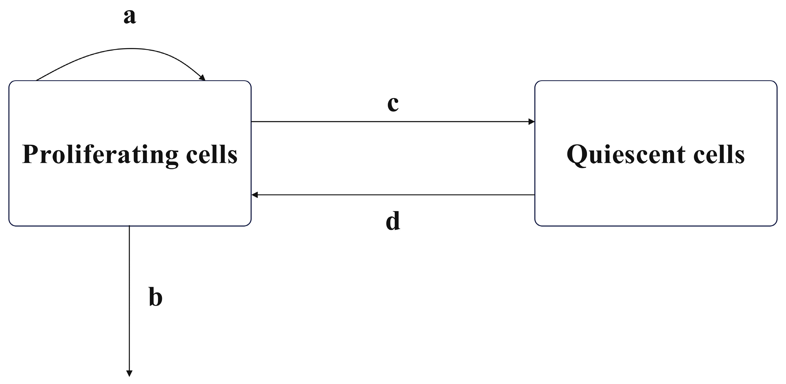
The combined cell cycle-specific and non-cycle-specific chemotherapy proposed in this paper is based on the linear tumor growth model of drug resistance and cell cycle specificity proposed by Panetta et al. [21,23] and further modified by Bharti Panjwani et al. [22]. All cells in the body undergo a series of proliferation stages involving division and replication during growth, which are divided into the interphase and the mitotic phase, with a resting phase indicating temporary cell inactivity. The interphase includes the gap phases G1, synthesis phase S, and gap phase G2, while the mitotic phase is mainly the M phase. The resting phase is denoted as G0. Cells synthesize proteins and genetic material during the interphase, divide into two daughter cells during mitosis, and do not undergo any proliferation during the resting phase. Chemotherapeutic drugs that target specific phases of the cell cycle typically exert their effects by interfering with cells in the M phase. When establishing mathematical models, cells in the interphase and mitotic phase are often collectively classified as proliferating cell populations (), while cells in the resting phase are modeled as quiescent cell populations (). In the absence of drug action, tumor cell growth can be modeled by a dual-compartment model, as shown in Figure 1.
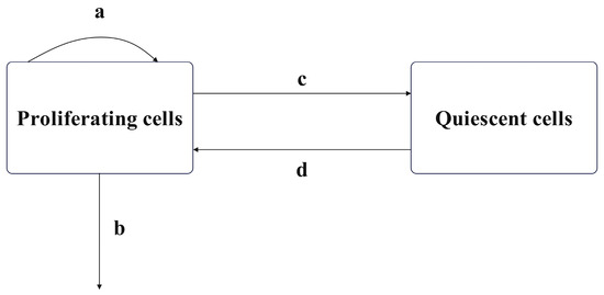
Figure 1.
Dual-compartment tumor model.
In Figure 1, a, b, c, and d, respectively, represent the natural growth rate of the proliferating cell population, the natural death rate of the proliferating cell population, the rate at which proliferating cells become quiescent, and the rate at which quiescent cells revert to proliferating cells. When using chemotherapy drugs, both the proliferating cell population and the quiescent cell population in the cell cycle-specific model may acquire resistance. The cell cycle-specific drug has no killing effect on the resistant cell population. According to this characteristic, the cell population can be further divided into drug-sensitive cell populations () and drug-resistant cell populations ().
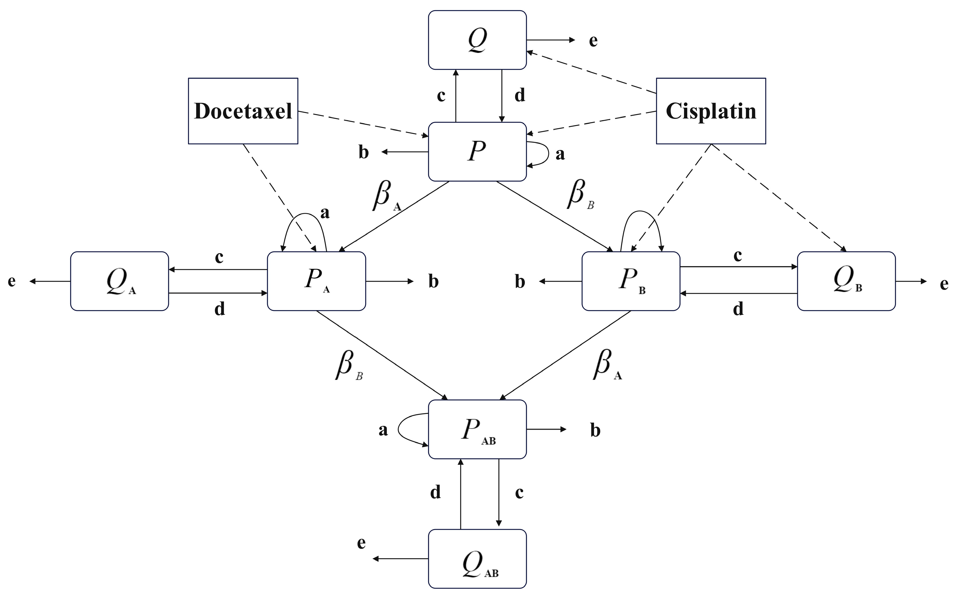
The model proposed in this paper focuses on the combination chemotherapy of cisplatin and docetaxel, with the non-cycle-specific drug cisplatin represented as Drug A in the model and the cycle-specific drug docetaxel represented as Drug B. The main variables of the model include tumor proliferating cells () and tumor quiescent cells () sensitive to both drugs; proliferating cells resistant only to cisplatin () and quiescent cells resistant only to cisplatin (), proliferating cells resistant only to docetaxel () and quiescent cells resistant only to docetaxel (), proliferating cells resistant to both drugs () and quiescent cells resistant to both drugs (), as well as bone marrow cells () significantly affected by the drugs. Quiescent cell populations and are affected by Drug A and have a certain probability of developing resistance, transferring to and . The total tumor cell population at the end of the treatment session and the cumulative damage to bone marrow cells are indicators of drug efficacy and toxicity levels in this model. As mentioned earlier, the modified linear tumor dynamics model consists of eight compartments, as shown in Figure 2, and can be represented by the following equations:
where t denotes time, denotes the unit step signal used to indicate that the drugs all have their efficacy appear after the first administration, and denote the instant of administration of the two drugs, and and denote the killing effect of the two drugs, respectively. The model describes tumor cell growth linearly due to chemotherapy’s efficacy in inhibiting growth near the carrying capacity. This linear kinetics simplifies calculations and offers transparency in interpreting underlying dynamics, particularly in the context of tumor growth dynamics. In the early stages of tumor growth, linear approximations provide a reasonable first-order approximation of the system’s behavior. Additionally, the effectiveness of chemotherapeutic routines in inhibiting tumor growth close to its carrying capacity suggests that any nonlinearity may have a negligible impact within our study’s scope. Furthermore, linear models often offer computational advantages, requiring fewer computational resources compared to nonlinear models, enabling faster simulations and facilitating exploratory analyses under various conditions. Our approach allows us to capture the fundamental dynamics of tumor growth without introducing unnecessary complexity. Unlike tumor cell growth, the bone marrow cell growth described in Equation (9) is formulated as a logistic equation, where denotes the natural growth rate of the bone marrow cell population, K denotes the carrying capacity of the bone marrow cell population, and the term denotes the amount of damage to the bone marrow cell population from exposure to the drug.
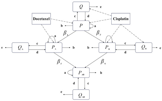
Figure 2.
Eight-compartments model.
The killing effect of drugs, denoted as and , depend on the rate of change in drug concentration at the tumor site, and the pharmacokinetic equation used in this model is shown in the following equation:
where and represent the drug doses injected into the patient’s body at time , its unit is mg/mL per day. and represent the drug concentrations at the tumor site, and represent the decay rates of the two drugs, and and are constants representing the killing effect of the drug concentration on cells per time unit.
The remaining tumor cells and the cumulative damaged bone marrow cell population are utilized as the two optimization objectives, and the solution of the TA-MOSSA represents the drug dosage regimen of the two drugs throughout the course of treatment. Objective1, representing the remained tumor cells, and Objective2, representing the cumulative damaged bone marrow cells, are calculated as shown in Equation (14) and Equation (15), respectively:
Both objectives are to be minimized in this paper, representing the efficacy and the toxicity levels of chemotherapy regimens, respectively.
Moreover, during the optimization process, constraints are imposed on the drug concentration within the patient’s body and the population of bone marrow cells [22] to avoid overdose. These constraints are reflected in the following equation:
Thus, penalty function is defined as in Equation (18), and, accordingly, Objective2 is modified as shown in Equation (19).
where denotes the penalty factor.
The parameters listed in Table 1 pertain to the model and are based on relevant literature sources [15,22,23,26,27,28,29,30,31].

Table 1.
Summary of model parameters.
3.2. Two-Archive Multi-Objective Squirrel Search Algorithm
3.2.1. Squirrel Search Algorithm (SSA)
The Squirrel Search Algorithm (SSA), introduced by Mohit Jain, Vijander Singh, and Asha Rani in 2019 [6], mimics the foraging behavior of flying squirrels. The SSA is inspired by how flying squirrels glide between trees to gather food during warm weather, while their activity reduces during cold weather until warmer seasons return. The SSA operates under the following assumptions: (1) The forest contains flying squirrels (FS), each located on a tree. (2) Each FS independently engages in dynamic foraging behavior. (3) The forest comprises one hickory nut tree, three acorn nut trees, and the remaining trees are normal.
The mathematical model for the SSA is constructed through the following steps:
- i.
- Random initialization
Each FS individual is denoted by a vector of length , which serves as an optimization solution. These vectors can be initialized from a uniform distribution, as described in Equation (20):
where denotes the dimension of flying squirrel and and represent the upper and lower bounds, respectively. The location of the flying squirrel population with the size of can be represented as the matrix shown in Equation (21):
- ii.
- Fitness evaluation and Ranking
The fitness function evaluates the fitness value of each individual’s location, ranking the flying squirrels accordingly. The individual with the best value is placed on the hickory nut tree (), while the next three individuals are assigned to acorn nut trees (), with the remaining squirrels assumed to be on normal trees.
- iii.
- Random selection of movement
Some individuals on normal trees glide towards the hickory nut tree for food storage, while others move towards the acorn nut trees. Additionally, three individuals on acorn nut trees move towards the hickory nut tree. Flying squirrels exhibit random avoidance behavior when encountering a predator, denoted by the probability .
- iv.
- Generate new locations
As described above, the dynamic foraging mechanism has three cases. It can be presented as the following equations:
Case 1.
Individuals on acorn nut trees () head for hickory nut tree (), new locations at iteration as represented in Equation (22):
where denote a random gliding distance, is a sliding constant to balance exploration and exploitation, is random within [0,1], represents the hickory nut tree position at iteration .
Case 2.
A small part of individuals on normal trees () proceed in the direction of acorn nut trees (), and their new locations at iteration can be represented as Equation (23):
where is random within [0,1].
Case 3.
The rest individuals on normal trees () head for the hickory nut tree (), and their new locations at iteration can be represented as Equation (24):
where is random within [0,1].
- v.
- Seasonal monitoring conditions
The foraging strategies employed by flying squirrels change seasonally, and they tend to move less in winter. Therefore, monitoring parameters are introduced for easing local optima stagnation. The seasonal constant and the minimum value of seasonal constant are calculated using Equation (25) and Equation (26), respectively. Subsequently, these two parameters are used to determine the season.
where t = 1, 2, 3.
where and denote current iteration numbers and maximum iteration numbers, respectively.
The seasonal monitoring condition is met when (i.e., winter has ended and summer comes). Flying squirrels on normal trees would be randomly relocated using the following Equation (27):
where Lévy Flight is applied for more efficient exploration, it can be calculated by Equations (28) and (29) below:
where and denote numbers within , is a constant number equaling to 0.5 and .
In contrast, means summer has not come yet, flying squirrels would not enforce any extra moving behavior. The pseudocode of the SSA is shown in Algorithm 1.
| Algorithm 1: Squirrel Search Algorithm |
|
3.2.2. Improved Two-Archive Algorithm (Two_Arch2)
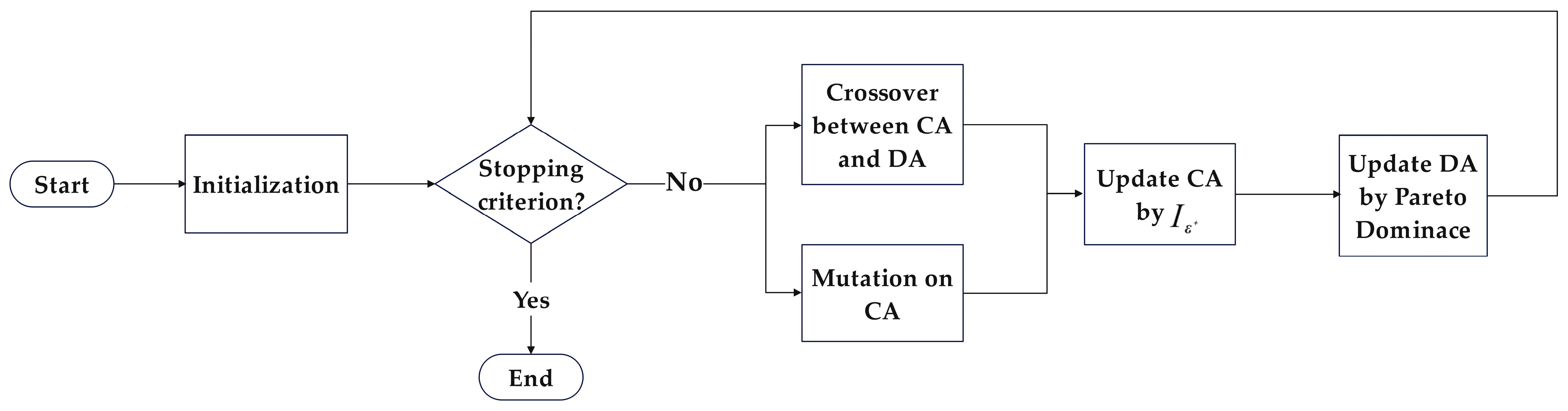
The Two-Archive Algorithm (TAA) is a multi-objective optimization algorithm proposed by Kata Praditwong and Xin Yao [32]. Unlike the common mechanism in multi-objective optimization, where a single external archive stores non-dominated solutions, TAA adopts a dual-archive preservation approach, assigning non-dominated solutions to either the Convergence Archive (CA) or the Diversity Archive (DA). This aims to simultaneously maintain the convergence and diversity of the obtained Pareto solution set, ensuring that the final solution set closely approximates the ideal Pareto front with a broad coverage range without introducing additional computational complexity to the algorithm. The TAA process is illustrated in Figure 3.
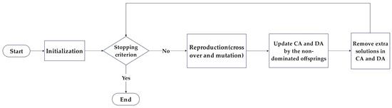
Figure 3.
Flowchart of TAA.
The Improved Two-Archive Algorithm (Two_Arch2) is a refinement proposed by Handing Wang et al. [33] to address the limitations of the TAA algorithm. Handing Wang et al. noted that, when the sum of the sizes of the two archives exceeds a predefined limit, only solutions from the Diversity Archive (DA) are pruned. If the size of the Convergence Archive (CA) reaches this limit, all solutions from the DA are removed. Additionally, the maintenance mechanism of the CA does not guarantee its diversity. As a result, the diversity of the final output Pareto solution set is greatly diminished. Two_Arch2 improves the updating mechanisms of both the CA and DA and independently limits the size of the two archives. During CA updating, all offspring solutions obtained are added to the CA, and then, based on an indicator-based fitness function proposed in [34], surplus solutions are removed. The fitness function, based on the quality indicator , constructs the minimum distance required for a solution to dominate another solution , expressed as follows:
where denotes the mth objective function and is the total number of objective functions.
Fitness function is defined as in Equation (31):
where represents the set of all solutions in set , except for , and the fitness function of solution is calculated by summing over all other solutions in the set. If the size of the CA exceeds the upper limit, the solution with the minimum fitness value is deleted during iteration, and the fitness function is recalculated based on the remaining solutions in the archive, repeating this deletion step until the size of the CA equals its upper limit.
The update of the DA is still based on dominance. Non-dominated solutions in the offspring population are directly added to the DA. If the size of the archive exceeds the upper limit, each solution in the DA is examined individually to determine whether it can be retained. Firstly, solutions with the maximum and minimum objective values on each objective function are retained, and the remaining solutions are then individually assessed for similarity during iteration. Similarity is measured by the distance between solutions in the objective space, with Two_Arch2 using the fractional distance (, p < 1). For two different solutions and , their fractional distance is expressed as follows:
where denotes the mth objective function and is the total number of objective functions, usually set . Similarity for solution is defined as in Equation (33):
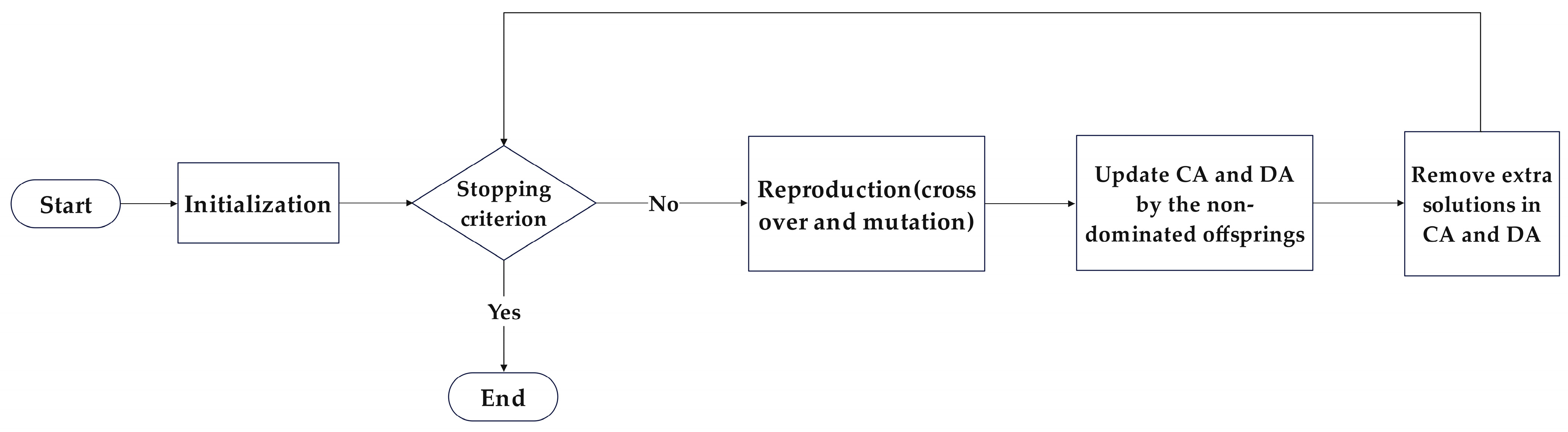
where represents the set of all solutions in set DA except for . When updating the DA, similarity among all solutions will be computed in each iteration, and the solution with the maximum similarity will be retained in the DA until the size of the DA reaches its limit. The Two_Arch2 process is illustrated in Figure 4.
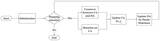
Figure 4.
Flowchart of Two_Arch2.
3.2.3. Two-Archive Multi-Objective Squirrel Search Algorithm (TA-MOSSA)
The primary issue in extending the Squirrel Search Algorithm (SSA) to the domain of multi-objective optimization lies in how to select the optimal solution. Due to the difficulty in obtaining a single optimal solution that dominates all other individuals in terms of all objective functions, it is also challenging to determine the fitness values of the hickory nut tree () and acorn nut tree () simply by comparing the objective function values. Common improvement methods in existing research on the multi-objective Squirrel Search Algorithm often involve introducing a single external archive mechanism from the Non-dominated Sorting Genetic Algorithm II (NSGA-II), determining and based on non-dominated ranks [35,36] or grid density [37]. However, considering the reason the SSA selects the optimal and suboptimal solutions as and , respectively, it is important to guide the convergence and diversity of the solution population separately during the search process. The optimal solution guides most of the population individuals to converge towards the optimal direction, while multiple suboptimal solutions ensure that the search space is thoroughly explored and the local optima are alleviated. A single external archive cannot effectively balance convergence and diversity. The functionality assigned to and in the SSA process essentially matches the functionality of the convergence archive (CA) and diversity archive (DA) in the Two_Arch2. Therefore, the proposed TA-MOSSA introduces the improved two-archive mechanism. In each iteration, new solutions are generated and used to update the two external archives, CA and DA, with the updated CA and DA serving as the candidates for and , respectively, in the next iteration.
The dynamic foraging mechanism of the SSA was also modified accordingly. Each of the individuals moving towards randomly select solutions as the target from CA, ensuring a broad balance between objectives and introducing some diversity into the convergence process while converging towards the ideal Pareto front, expanding the coverage range of the Pareto solution set. The individuals moving towards accordingly randomly select solutions from the DA.
For the new solutions generated from the dynamic foraging mechanism, each is updated based on the greedy principle and dominance relationship. Let be the new solution generated after ’s gliding; if dominates , replaces ; if they have no dominance relationship, and replaces with a certain probability, ensuring that the progresses towards the ideal Pareto frontier in each iteration of the search process while further introducing variability into the population. The above updating rule can be expressed as Equation (34):
where and , respectively, denote the previous and current iterations within the search process.
The pseudocode for the dynamic foraging mechanism in the TA-MOSSA, improved based on the two-archive mechanism, is presented in Algorithm 2.
| Algorithm 2: Improved dynamic foraging mechanism of TA-MOSSA |
Initialization: The number of max iterations , initial iteration , convergence archive CA, divergence archive DA
|
In the original Squirrel Search Algorithm (SSA), the seasonal monitoring condition serves to evaluate overall convergence and determine whether the search process should prioritize global exploration or local exploitation. During “summer”, the SSA infers that the solution population is nearing convergence. It then randomly relocates all individuals to promote global exploration and prevent premature convergence to suboptimal solutions. Conversely, in “winter”, the SSA maintains the current status and allows individuals to continue moving towards or . As shown in Equation (19), the seasonal monitoring condition emphasizes global search in the early stages and local exploitation in the later stages of algorithm iterations, achieving an adaptive balance between the two. However, since the multi-objective optimization generates a set of non-dominated solutions, the seasonal monitoring conditions described in Equation (19) are insufficient for capturing the convergence of the Pareto front during the search process. Therefore, we introduce the generation gap (G) [37] to modify the seasonal monitoring conditions in the proposed TA-MOSSA. The generation gap (G) is an indicator used in evolutionary algorithms to measure the convergence of the population. It quantifies the convergence of the population by calculating the minimum Euclidean distance between all non-dominated solutions generated in two consecutive iterations, expressed as follows:
where represents the minimum Euclidean distance between the ith non-dominated solution at the iteration and all non-dominated solutions generated at the iter iteration. denotes the non-dominated solution, and and are the number of non-dominated solutions generated in the and iter iterations, respectively. A smaller generation gap value indicates that the newly generated non-dominated solution set shows no significant change compared to the previous iteration, indicating that the search process tends towards local exploitation and gradually converges. A larger generation gap indicates a significant difference between the non-dominated solution sets obtained in two consecutive iterations, indicating that the algorithm’s search process has not yet reached a stable convergence state. In this case, the calculation of the minimum seasonal constant value remains unchanged to preserve the adaptive balance between global exploration and local exploitation, as in the original SSA. The calculation of the minimum seasonal constant remains unchanged, as in Equation (20), to preserve the adaptive balance between global exploration and local exploitation.
To help the search process converge better towards regions with superior solutions, the two-point crossover operator is introduced to the seasonal monitoring mechanism, serving as a local search for solutions in the Convergence Archive (CA). This improvement fully utilizes the neighborhoods of CA solutions to explore potential better solutions. Solutions are then selected and replaced based on dominance relations, enhancing the quality of the Pareto front and alleviating local optima to some extent.
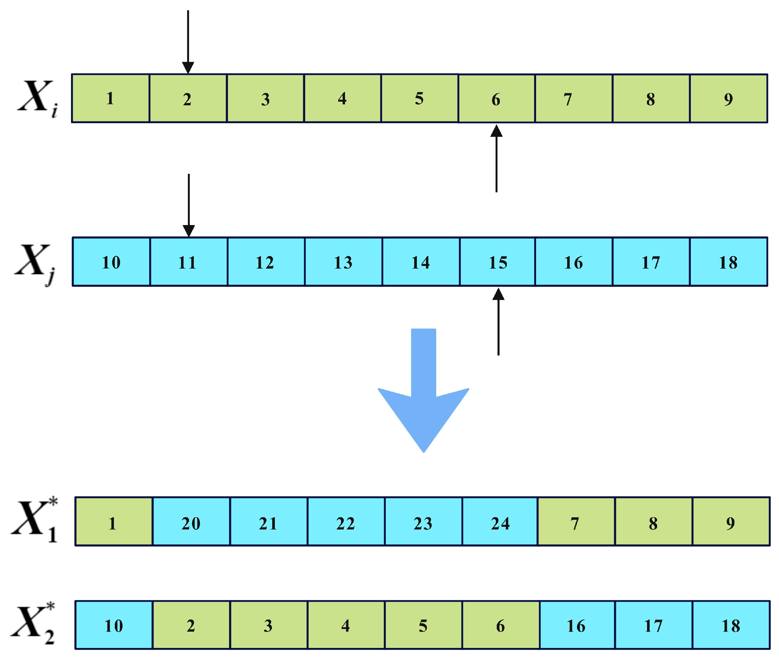
The two-point crossover operator, a widely employed method in genetic algorithms, generates offspring by recombining parental genetic information. The primary steps involved are as follows:
- Randomly selecting two crossover points within the chosen parent individuals, dividing them into three segments. These crossover points are the same for both parental individuals.
- Exchanging segments between the crossover points of parental individuals to produce two new offspring individuals.
The implementation of the two-point crossover is illustrated in Figure 5, where and represent the parent solutions, the arrow indicates the crossover point, and and represent the offspring. It can be observed that the two-point crossover operator introduces relatively small and concentrated variations in individual solutions. Employing the two-point crossover operator for local search facilitates exploration of neighborhoods surrounding optimal solutions, preserving their vital information. This contributes to a finer balance between global exploration and local exploitation.

Figure 5.
Two-point crossover operator.
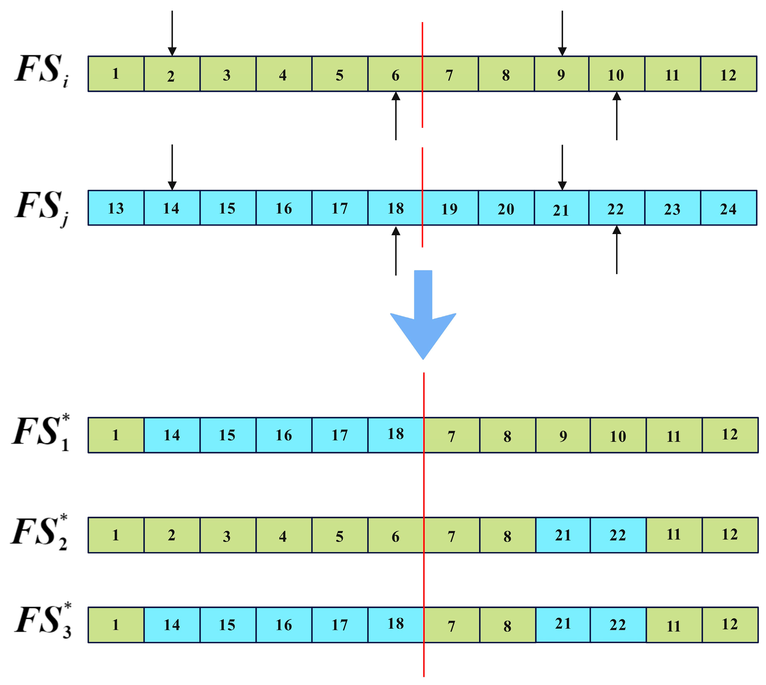
For the multi-objective combined chemotherapy dosing optimization, each solution represents a dosage plan for chemotherapy, structured as a vector of length The first elements and the last elements, respectively, represent the dosage plans for drug A and drug B throughout the entire treatment session. When applying the two-point crossover operator, the process of generating neighbor solutions is illustrated in Figure 6, where the red lines indicate the division of the dosage plans for drugs A and B within the solution. represents the ith solution selected from the CA during the iteration, while represents any solution different from in the CA. , , and represent the neighbor solutions generated by two-point crossover, and the new generated solutions are all based on . is then replaced by a random non-dominated solution from set {, , , } if there is dominance relation among them; otherwise, an is replaced by a random one of them.
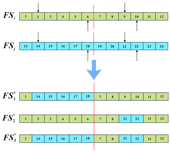
Figure 6.
Two-point crossover of dosage plan.
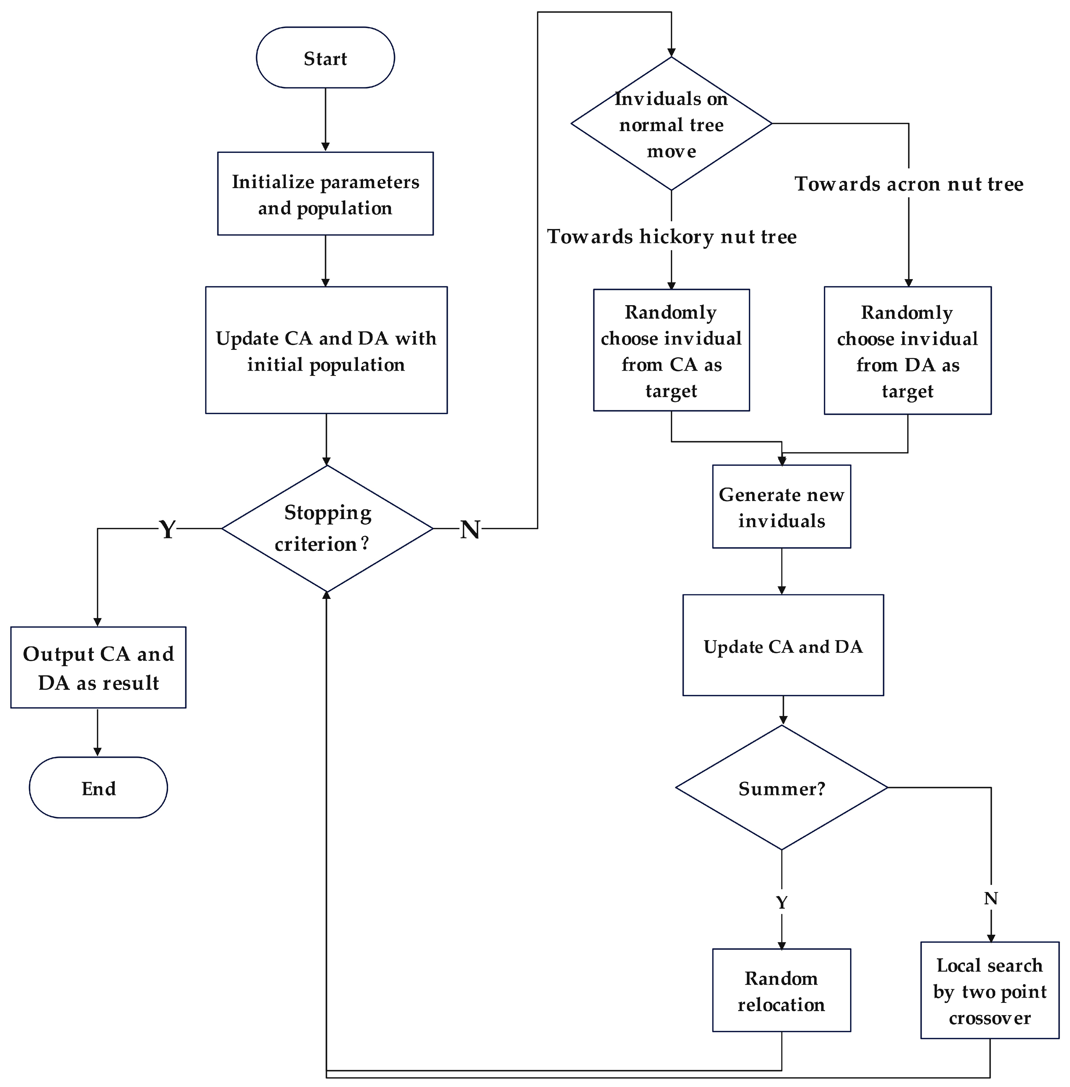
The flowchart of the proposed TA-MOSSA is given in Figure 7.
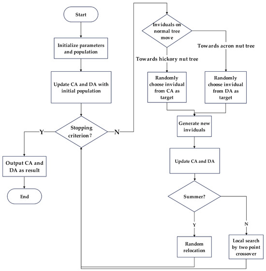
Figure 7.
Flowchart of proposed TA-MOSSA.
4. Experimental Setup and Results Analysis
4.1. Experimental Setup
To evaluate the performance of the proposed TA-MOSSA algorithm in the optimization of chemotherapy dosing, the experiment applies it to patients simulated by a tumor growth model and compares the chemotherapy plans obtained with other multi-objective algorithms. For two different treatment scenarios, chemotherapy regimens are selected from the non-dominated solution set by considering different trade-offs in optimization objectives to compare their efficacy. Scenario 1 represents a more aggressive chemotherapy regimen, prioritizing tumor reduction and disease control, typically used in curative chemotherapy aimed at eradicating the tumor. It is suitable for patients in the early stages of cancer or for those without other medical conditions and with optimistic health conditions. Scenario 2 represents a milder regimen, prioritizing patient quality of life and comfort. Compared to the first scenario, the mild regimen minimizes bone marrow damage and is suitable for palliative chemotherapy aimed at relieving symptoms for late-stage patients or those with severe complications to prolong survival.
In this context, the experimental results are expected to be in silico, as the evaluation is conducted using computational simulations rather than real-world experiments.
The multi-objective algorithms compared in this study include classic algorithms that have been widely used in optimizing chemotherapy doses in recent years, such as the Non-dominated Sorting Genetic Algorithm II (NSGA-II) [4,13,22], the Multi-Objective Particle Swarm Optimization Algorithm (MOPSO) [13,16,38], as well as the improved Two Archive algorithm (Two_Arch2) [33], the Constrained Two-Archive Evolutionary Algorithm II (C-TAEA-II) [39] for constrained multi-objective optimization, and the original Multi-Objective Squirrel Search Algorithm (MOSSA) [37]. The latter three are included to illustrate the performance improvements of the TA-MOSSA. Algorithms involved are implemented with Python 3.9, and all experiments are performed on an Intel Core 2.30 GHz CPU with 16 GB of RAM and Windows 11 version 21H2 system. The implementation of the algorithms was carried out using PyCharm 2022.1.1 (Community Edition).
Moreover, robustness experiments were conducted to showcase the applicability of the proposed TA-MOSSA algorithm across patients with diverse tumor growth conditions and to evaluate the algorithm’s robustness. Various tumor growth scenarios were simulated by systematically adjusting the parameters of the tumor growth model.
4.2. Performance Metrics
In addition to the optimization objectives expressed in Equations (14) and (15), the performance of the proposed TA-MOSSA is also evaluated using the Hypervolume (HV) [36,40] and Spacing Metric (SP) [41] and compared with other multi-objective algorithms.
Hypervolume (HV) is a widely used performance metric for evaluating multi-objective algorithms. A larger hypervolume value indicates a better coverage of the objective space by the solution set, and thus higher solution quality. HV can be calculated using the following equation:
where denotes the set of non-dominated solutions, and represents one of the non-dominated solutions, refers to a reference point in the target space, and denotes the Lebesgue Measure, which is utilized to measure the size or volume of a set in Euclidean space.
The Spacing Metric (SP) is employed to measure the standard deviation of the minimum distance between each solution in the non-dominated solution set and other solutions. This metric reflects the uniformity of the distribution of the solution set, where a smaller SP value indicates a more uniform distribution. SP can be calculated using the following equation:
where denotes the set of non-dominated solutions and denotes the number of solutions in it, while is the minimum Euclidean distance between the ith solution and other solutions and is the mean value for all .
4.3. Parameter Analysis
In this section, Taguchi Method is utilized to determine the values of three important hyperparameters: the number of iterations (Itr), population size (NP), and penalty factor (), with the Hypervolume (HV) serving as the response variable (RV). The four levels for each parameter are presented in Table 2. The orthogonal array is selected for analysis, as outlined in Table 3. The results of the Taguchi analysis are given in Table 4, which includes the Delta values and significance rankings for each parameter. Based on the results, the chosen hyperparameter values are as follows: Itr = 100, NP = 150, and .
Table 2.
Parameter level.
Table 3.
Orthogonal array .
Table 4.
Mean response variable and significant rank.
4.4. Results and Analysis
4.4.1. Comparison of Overall Performance
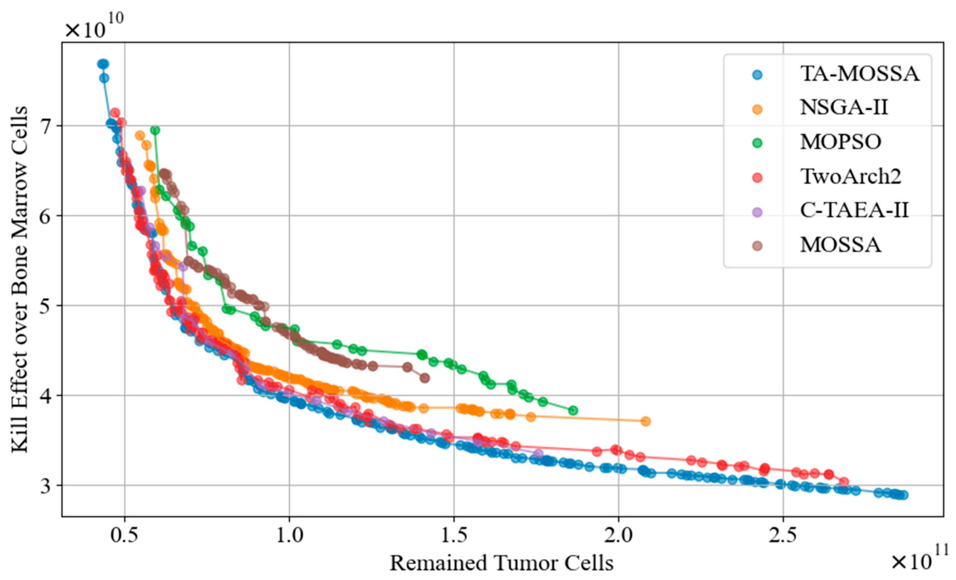
The performance metrics hypervolume (HV) and Spacing Metric (SP) are used to compare the overall performance of the TA-MOSSA and other algorithms in terms of the Pareto front obtained. Figure 8 displays the Pareto fronts of all algorithms. To mitigate the impact of the inherent randomness of meta-heuristic optimization algorithms on the experimental results, each algorithm is independently executed 30 times, and the mean HV and SP values across all runs are taken as the final experimental results. The optimal results are highlighted in bold in Table 5.
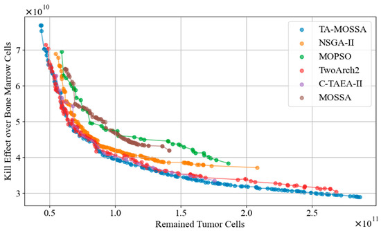
Figure 8.
The Pareto front of all algorithms.
Table 5.
Performance metrics of Pareto fronts.
Analysis of Figure 8 reveals that the Pareto front generated by the TA-MOSSA exhibits the widest coverage among all compared algorithms. It closely aligns with the Pareto fronts of Two_Arch2 and C-TAEA-II in the objective space, indicating that algorithms featuring a dual-archive mechanism excel in chemotherapy optimization. Conversely, the Pareto fronts obtained by MOPSO and the MOSSA are notably higher and exhibit narrower coverage, suggesting suboptimal optimization performance. Notably, in the objective of minimizing bone marrow cell damage, the disparity in damage between the optimal solutions of MOSSA and the TA-MOSSA exceeds cells, underscoring the substantial performance enhancement achieved by the TA-MOSSA over the MOSSA’s utilization of a single external archive mechanism.
Moreover, according to Table 5, the TA-MOSSA outperforms other algorithms across both performance metrics. While MOPSO demonstrates the highest SP value, the MOSSA exhibits the smallest HV value among all algorithms, aligning with the characteristics illustrated by the Pareto front visualized in Figure 8. A higher HV value signifies that the Pareto front obtained by the TA-MOSSA boasts superior diversity, capturing a broader spectrum of trade-offs between conflicting optimization objectives. This offers a richer array of candidate chemotherapy regimens for medical decision-making, showcasing the TA-MOSSA’s robustness in the search process. Conversely, a smaller SP value indicates a more uniform distribution of non-dominated solutions on the Pareto front, indicating the TA-MOSSA’s thorough exploration of the objective space.
4.4.2. Aggressive Chemotherapy Regimen
In this subsection, we compare aggressive chemotherapy regimens, specifically selecting those with the smallest remaining tumor cell counts for comparison. Table 6 presents the indicators obtained during the treatment process for each algorithm’s regimen, while Figure 9 depicts the trends in tumor cell and bone marrow cell counts over the treatment period.
Table 6.
Performance metrics of aggressive chemotherapy treatment.

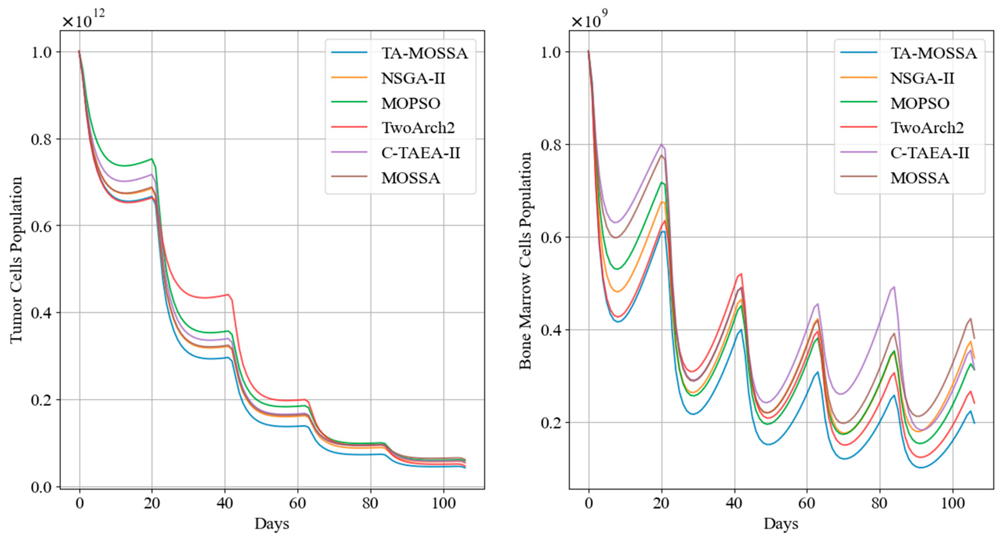
Figure 9.
Tumor cell and bone marrow cell population dynamics during aggressive chemotherapy treatment.
The results in Table 6 indicate that the chemotherapy regimen obtained by the TA-MOSSA employs a high drug dosage, resulting in the maximum reduction in tumor cells, with only 4.30% of tumor cells remaining. This underscores a prioritization of minimizing the remaining tumor cell count as the optimization objective, despite leading to the highest level of bone marrow cell damage ). Moreover, this aggressive regimen does not violate the constraints expressed in Equation (6), with the minimum bone marrow cell count during chemotherapy being . This indicates effective tumor reduction while keeping damage to normal cell tissues within acceptable limits.
Among the other chemotherapy regimens, the regimen produced by the TwoArch2 algorithm exhibits a performance similar to that of the TA-MOSSA regimen across various performance indicators, with a residual tumor cell proportion of 4.69%. However, the remaining tumor cells after treatment in the remaining chemotherapy regimens are relatively higher compared to the aforementioned regimens. Although these regimens result in lower cumulative bone marrow cell damage, they demonstrate less superiority as aggressive regimens compared to the regimen generated by the TA-MOSSA.
Additionally, Figure 9 highlights that, following the initial medication administration, the tumor cell count in patients treated with the chemotherapy regimen corresponding to TA-MOSSA remains consistently lower compared to other regimens.
4.4.3. Mild Chemotherapy Regimen
In this subsection, we compare the chemotherapy regimen with the smallest cumulative bone marrow cell damage. Table 7 outlines the indicators obtained during the treatment process for each algorithm’s chemotherapy regimen, while Figure 10 illustrates the trends in tumor cell and bone marrow cells over treatment sessions.
Table 7.
Performance metrics of mild chemotherapy treatment.
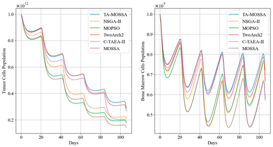
Figure 10.
Tumor cell and bone marrow cell population dynamics during mild chemotherapy treatment.
As indicated in Table 7, the mild chemotherapy regimen obtained by the TA-MOSSA maintains relatively low concentrations of cisplatin and docetaxel within the patient’s body, lower than those of other chemotherapy regimens. Moreover, it incurs the least cumulative damage to bone marrow cells, totaling only cells. This ensures that, even at the lowest point during the entire treatment course, there are still cells present in the bone marrow cell population, with an average level of cells. In contrast, the lowest points in bone marrow cell counts for the remaining chemotherapy regimens are all below 50% of the initial values. The chemotherapy regimen obtained by the MOSSA, with the lowest efficacy, corresponds to a bone marrow cell count at its lowest point, close to 40%, similarly failing to demonstrate a good balance in conflicting optimization objectives and adequate consideration for protecting the bone marrow cell population.
Additionally, Figure 10 indicates that the chemotherapy regimen obtained by the TA-MOSSA ensures that the bone marrow cell count remains higher than that of other chemotherapy regimens after each administration while still achieving significant tumor reduction, with only 28.64% of residual tumor cells. Conversely, the chemotherapy regimens obtained by MOPSO and the MOSSA result in substantial damage to bone marrow cells after two administrations between the 40th and 80th days, with a drop in bone marrow cell population approaching This significantly impacts patient health and contradicts the original intention of mild chemotherapy regimens to ensure a high quality of life for patients.
4.4.4. Comparison Study with Mathematical Models
In this subsection, we compared our proposed tumor dynamic model with the existing literature, including a dynamic model of cell cycle-specific drug combination chemotherapy [22] and a two-compartment cell cycle-specific model with a single drug [20,42], to demonstrate and validate the efficacy of our proposed model. These comparisons were made based on proliferating and quiescent tumor cell reduction proportions and remaining bone marrow cells under aggressive chemotherapy scenarios. The results of these comparisons are listed in Table 8.
Table 8.
Comparison of proposed model with models from the literature.
In Table 8, the proposed model of non-cycle-specific and cycle-specific combination chemotherapy demonstrates superior treatment efficacy compared to single-drug and cycle-specific combination chemotherapy under the aggressive chemotherapy scenario. T5he aggressive regimen from the proposed model achieves reductions in proliferating and quiescent cells of 95.87% and 95.65%, respectively, while resulting in a higher number of remaining bone marrow cells post-chemotherapy. Conversely, results from the literature [20], which utilized only one chemotherapy drug, exhibit the least promising treatment effect among all works. Furthermore, compared to the model of two cycle-specific drugs in combination chemotherapy, the regimen from the proposed model demonstrates significantly greater reductions in tumor cells. Specifically, the reduction proportion of proliferating cells from the proposed model exceeds that of the two cycle-specific drugs regimen by 2.92%, with a corresponding difference of 6.21% for quiescent cells. These findings suggest that both combination chemotherapy and the inclusion of a non-cycle-specific drug can significantly improve treatment efficacy and reduce side effects when compared to single-drug regimens. The validation of our model’s performance through this comparison study underscores its potential utility in optimizing chemotherapy regimens for enhanced therapeutic outcomes. In addition to the comparisons conducted in this study, future validation efforts will involve integrating clinical data to further refine and validate our model’s predictions against real-world observations.
4.4.5. Robustness Analysis
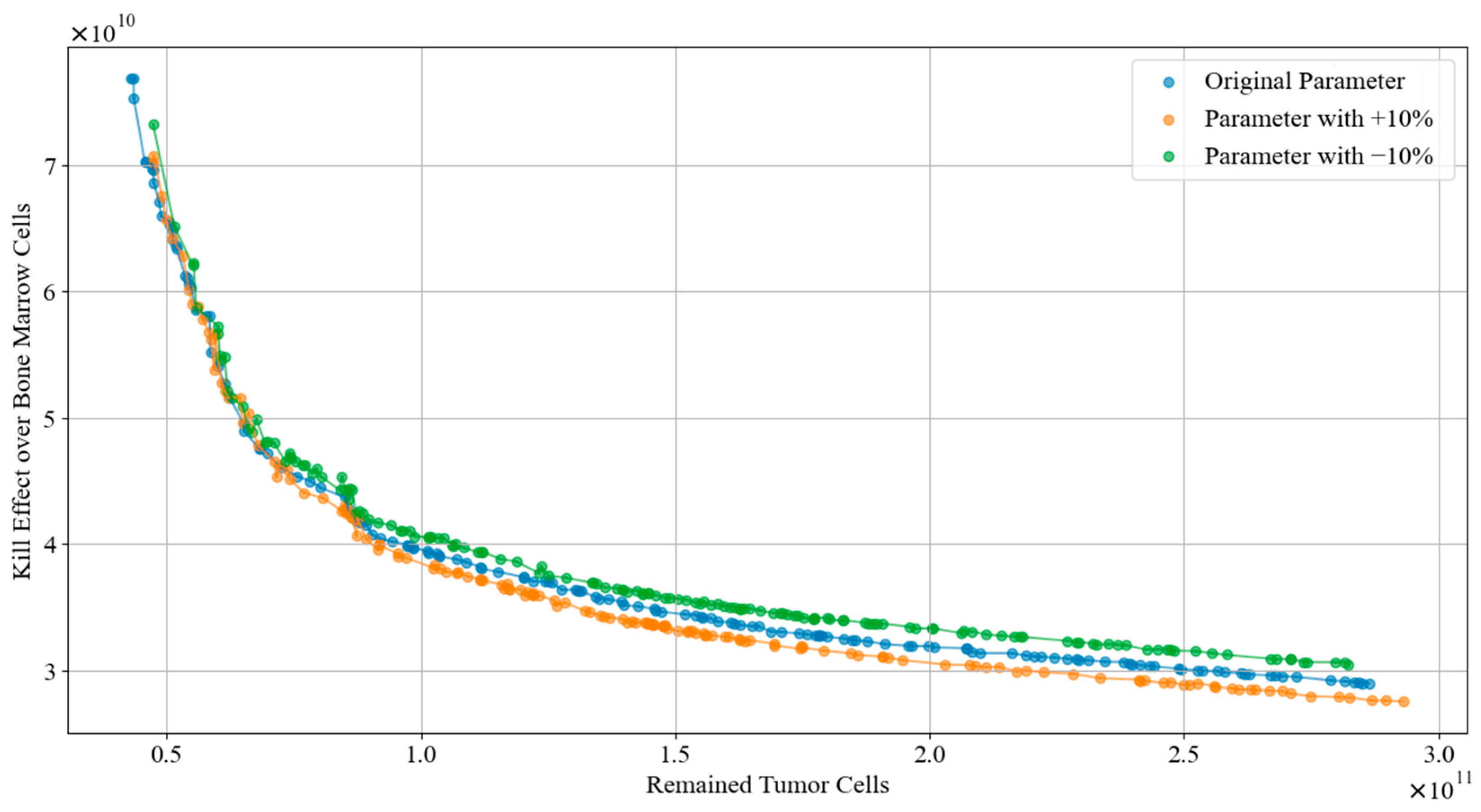
In this subsection, a robustness analysis is reported. We simulated various patients by adjusting the parameters of tumor dynamics model listed in Table 9. Subsequently, we applied the TA-MOSSA to generate the chemotherapy regimens of each condition. Figure 11 visualized the Pareto front curves obtained for the original parameters, as well as those increased by 10% and decreased by 10%. Furthermore, Table 9 offers comprehensive performance metrics, including the Hypervolume (HV) and Spacing Metric (SP), for each of the three parameter conditions.
Table 9.
Performance metrics of the Pareto fronts.
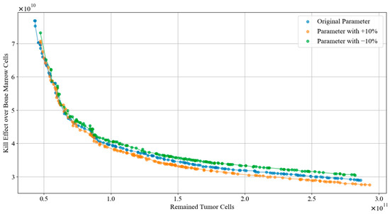
Figure 11.
Pareto front curves of different parameters condition.
Drawing from Figure 11 and Table 9, the Pareto front curves derived from altered parameters exhibit consistent trends and distribution of solutions. Notably, the curve corresponding to a −10% parameter adjustment maintains a similar overall value range to the original parameter curve in the objective space, while the curve with a +10% parameter adjustment shows a slightly reduced range. In the area where the number of remained tumor cells is minimal, all three Pareto front curves closely align, suggesting the proposed algorithm consistently excels in devising chemotherapy regimens that notably reduce tumor cells regardless of parameter variations. Furthermore, the fluctuations in HV and SP values of the Pareto fronts before and after parameter adjustments remain within 1%. This stability underscores the algorithm’s ability to sustain optimal coverage and even distribution of the Pareto frontiers despite parameter fluctuations.
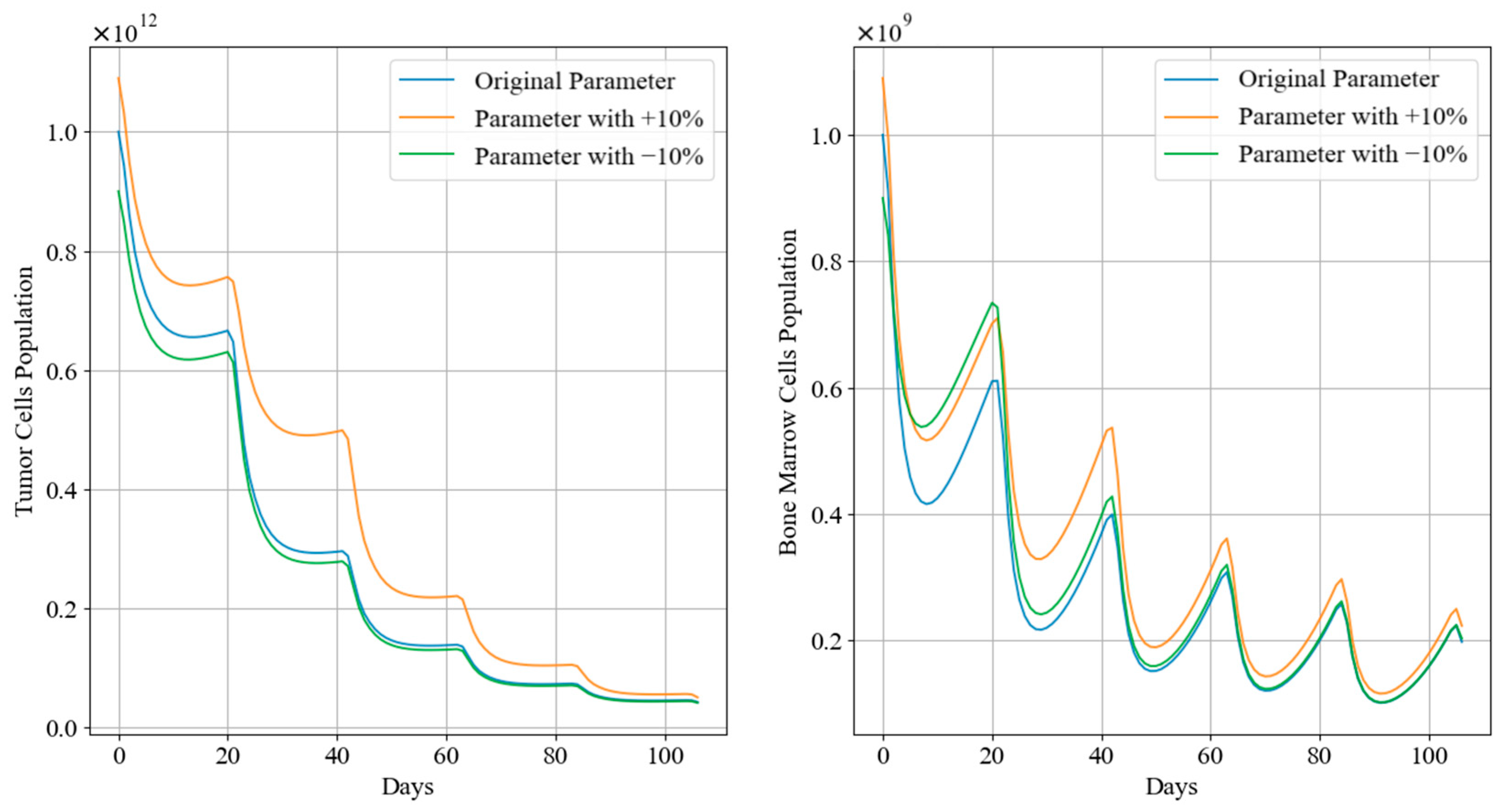
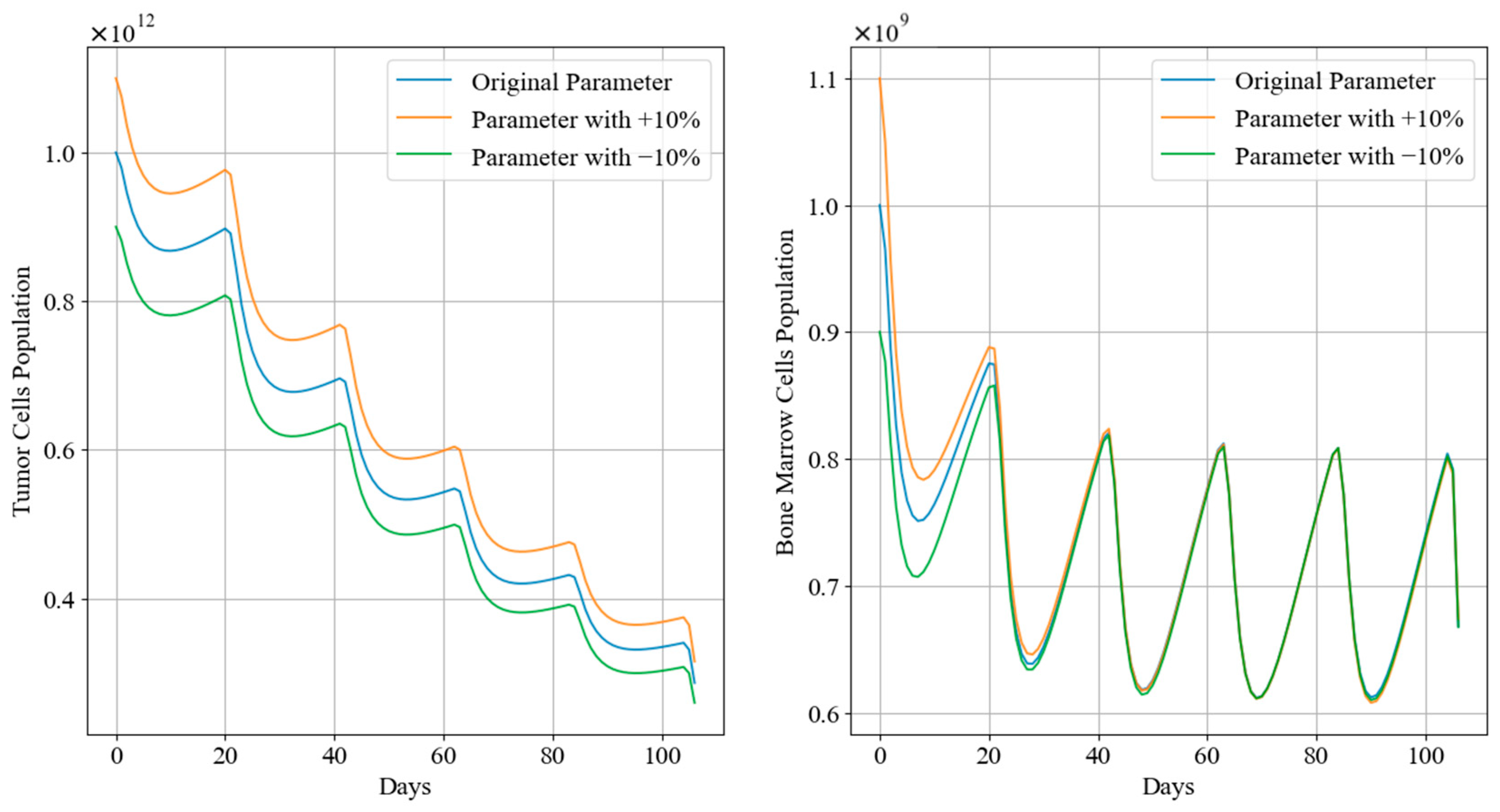
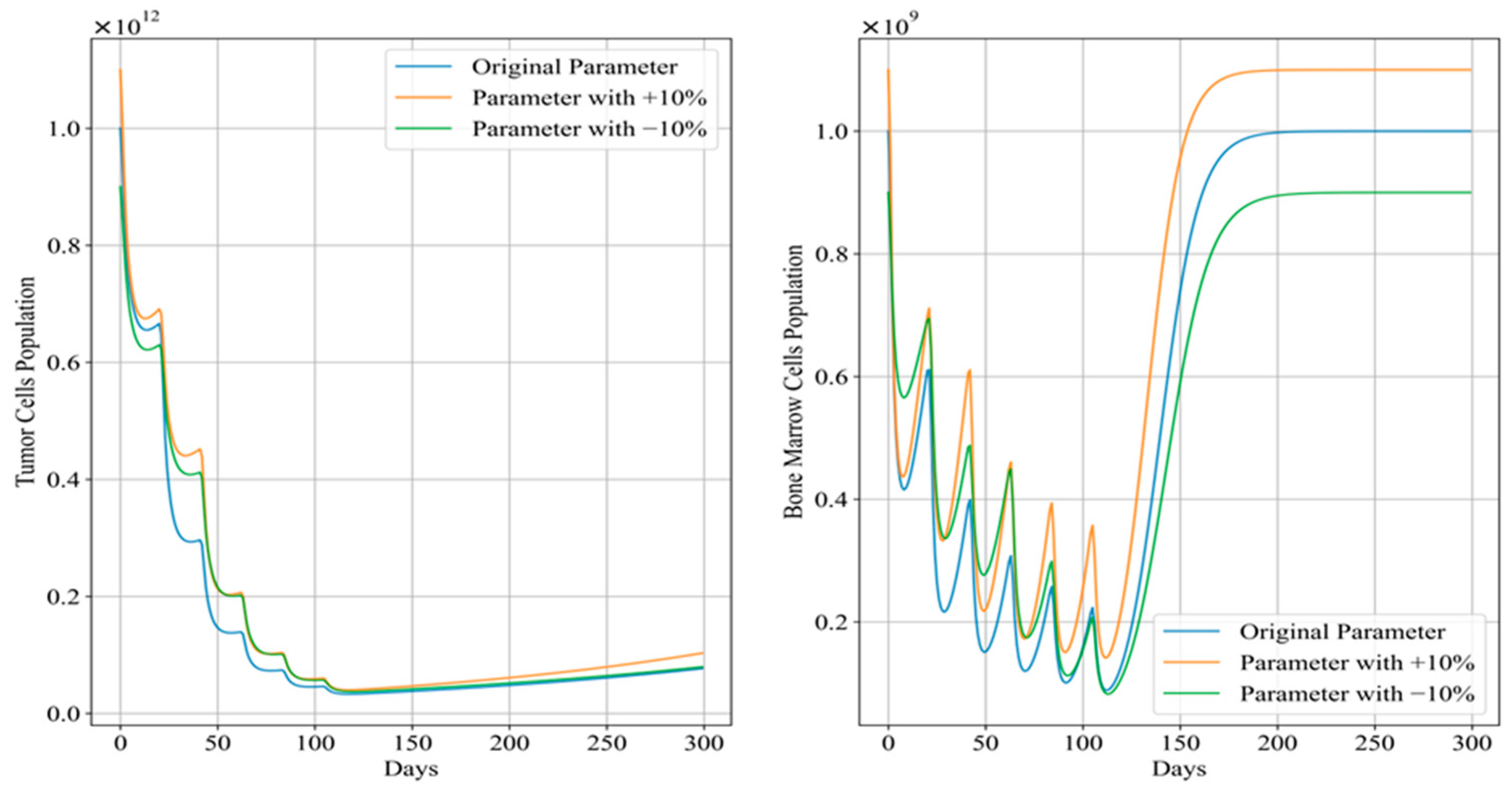
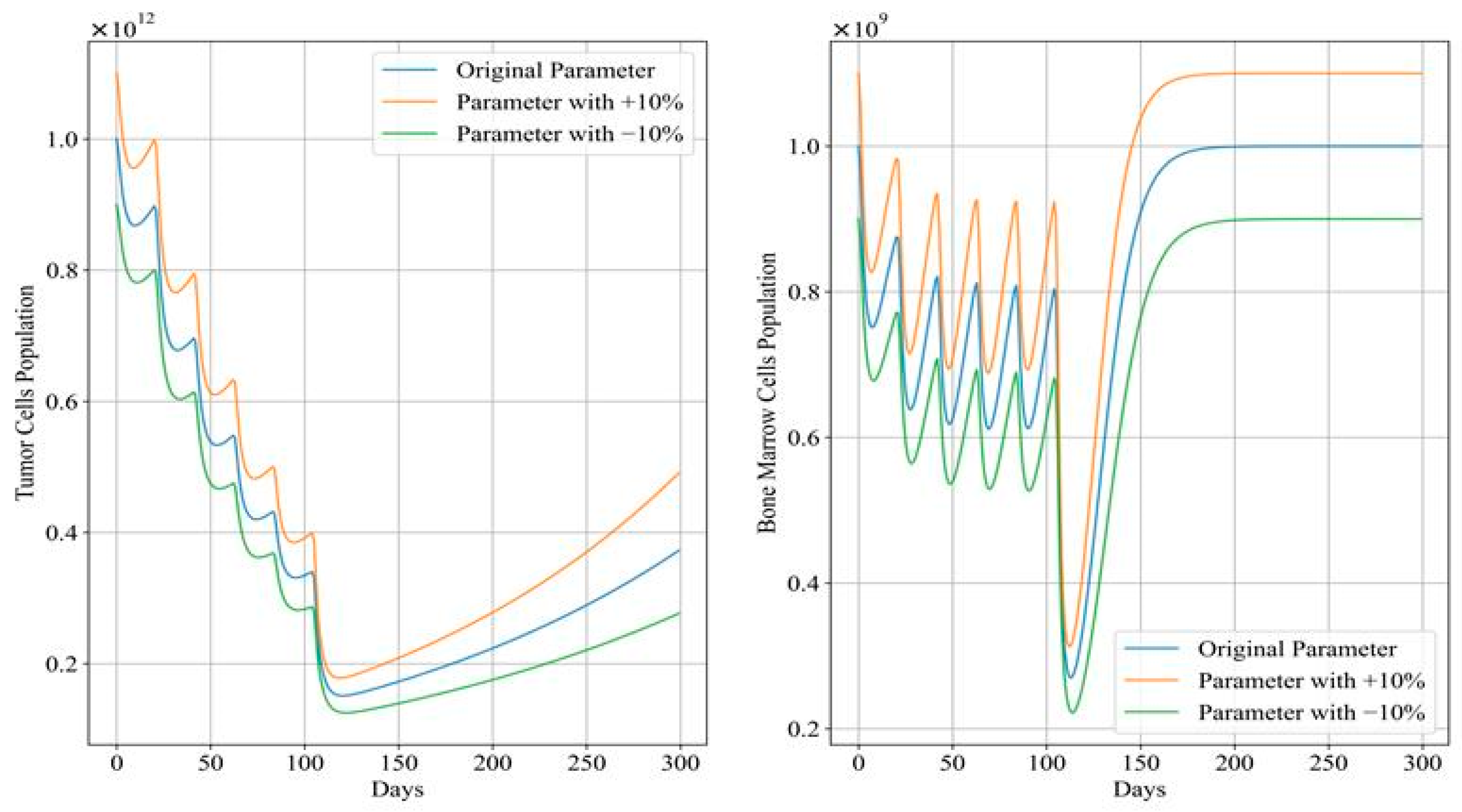
Figure 12 and Figure 13 depict the trends in tumor cell and bone marrow cell populations during aggressive and mild chemotherapy under different parameter conditions, respectively. The efficacy indicators of each chemotherapy regimen are reported in Table 10 and Table 11. Figure 14 and Figure 15 depict the long-term dynamics of both scenarios for up to 300 days, while the last doses are given at day 105 and day 106.
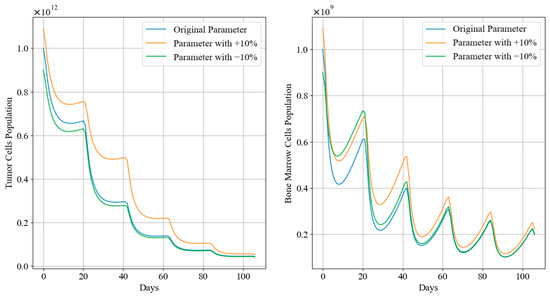
Figure 12.
Tumor cell and bone marrow cell population dynamics during aggressive chemotherapy treatment.
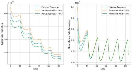
Figure 13.
Tumor cell and bone marrow cell population dynamics during mild chemotherapy treatment.
Table 10.
Performance metrics of aggressive chemotherapy treatment. under different parameter conditions.
Table 11.
Performance metrics of mild chemotherapy treatment under different parameter conditions.
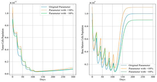
Figure 14.
Long-term dynamics of tumor cell and bone marrow cell population after aggressive chemotherapy treatment.
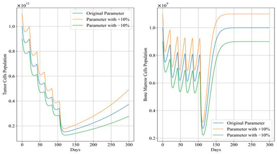
Figure 15.
Long-term dynamics of tumor cell and bone marrow cell population after mild chemotherapy treatment.
It can be observed that, during aggressive chemotherapy, although the +10% parameter regimen shows a smaller decrease in tumor cell count in the early stages of treatment, ultimately the chemotherapy regimens under all three parameter conditions achieve similar reductions in tumor cells, with remaining tumor cell proportions of 4.30%, 4.96%, and 4.19%, respectively, mirroring the characteristics of the Pareto front curves shown in Figure 11. The corresponding drug concentrations for all three chemotherapy regimens remain relatively high, with minimal differences in cumulative bone marrow cell damage and minimum bone marrow cell values. It is worth noting that the number of remained cells of the +10% parameters scenario is significantly higher than in the other two scenarios. In terms of clinical significance, +10% and −10% scenarios denote larger and smaller initial tumor sizes before any treatment is applied, and the algorithm TA-MOSSA optimized chemotherapy treatment accordingly. Furthermore, the +10% scenario tumor also grows faster than others, indicating a less favorable prognosis for patients under these conditions. Therefore, the larger number of remaining tumor cells observed in the +10% parameter scenario indicates that, even when feasible treatment is applied, larger tumor and higher growth rates still result in more remaining cells. However, it is obvious that the difference over the number of remained tumor cells among these parameter scenarios is quite slight, indicating the algorithm’s ability and robustness over varying parameters to optimize treatment plans based on varying patient parameters under the situation of non-cycle-specific and cycle-specific combination chemotherapy, efficiently addressing different tumor sizes and conditions; it may also be more efficient for larger tumor situation.
Drawing from Figure 14, after aggressive treatment, the tumor cell levels are quite low and remain low for a long time without further doses. On the other hand, bone marrow cells quickly rebound to levels near the carrying capacity.
During mild chemotherapy, the trends in tumor cell and bone marrow cell populations generated by the chemotherapy regimens under different parameter conditions exhibit similar patterns; however, there are slight differences in the endpoints of the tumor cell count change curves, with the maximum difference of approximately , indicating a close level of similarity. Regarding the bone marrow cell population, following the initial dose of the −10% parameter regimen, there is a sharp drop observed in its bone marrow cell population, distinguishing it from the other regimens. However, from day 20 of treatment until the end of the treatment period, all three trends stabilize at similar levels. Additionally, cumulative bone marrow cell damage and average values remain consistent, while drug concentrations show minor fluctuations within a small range, with the maximum difference not exceeding 0.03. Referring to Figure 15, in the case of mild treatment, the tumor cell levels rise faster than in the aggressive treatment scenario within a period after chemotherapy is completed. Meanwhile, bone marrow cells gradually return to levels near the carrying capacity, comparatively.
Based on the results of the robustness experiment described above, it can be concluded that the proposed TA-MOSSA can provide effective chemotherapy regimens for patients with different conditions, demonstrating robustness and reliability in both aggressive and mild chemotherapy scenarios.
5. Conclusions
The focus of this study is on the precise dose optimization of chemotherapy involving the non-cycle-specific drug cisplatin and the cycle-specific drug docetaxel. We modified the tumor growth model for cycle-specific drug combination chemotherapy to better suit this topic, taking into account acquired drug resistance and toxic side effects on bone marrow cell populations. We proposed a multi-objective Squirrel Search Algorithm named the TA-MOSSA, improved with a dual external archive mechanism and a local search mechanism, for analyzing chemotherapy regimen formulation in two different chemotherapy scenarios. The two-archive mechanism maintains the diversity and convergence of the population in the dynamic foraging mechanism of the Squirrel Search Algorithm, while the use of a local search in season monitoring mechanism effectively helps the search process approach the ideal Pareto front and achieve a superior Pareto solution set. Experimental results demonstrate that, compared to other multi-objective optimization algorithms, the TA-MOSSA generates a more diverse, evenly distributed, and broader coverage Pareto solution set, covering a wide range of trade-offs between conflicting objectives. Comparative experiments on the chemotherapy regimen selection based on different treatment strategies (aggressive and mild chemotherapy) show that the TA-MOSSA provides more comprehensive and effective candidate chemotherapy regimens for medical decision-making.
It is important to note that our study primarily serves as decision-making support for clinicians rather than a direct clinical study. As a mathematical model, our results offer insights into the potential efficacy of different treatment regimens and can inform clinical decision-making processes. Whether the optimized treatment plan can be applied to clinical requires the ultimate validation and implementation of these findings in clinical practice, requiring in vivo and further empirical validation and consideration of additional factors beyond the scope of our model. Another limitation of our study lies in the simplification of the biological system using a linear model. While linear models offer transparency and ease of interpretation, they inherently simplify the complex dynamics of biological systems. As a result, the applicability of our findings to clinical studies may be limited by the assumptions and constraints imposed by the linear model.
Moving forward, we recognize the need for further research efforts to validate our model against clinical data and to consider additional objectives, such as treatment duration and drug cost. These efforts will enhance the applicability and effectiveness of our chemotherapy optimization framework in real-world clinical settings. Furthermore, our commitment to collecting clinical data and conducting further testing underscores our dedication to refining and validating our model for practical application in clinical settings.
Author Contributions
Conceptualization, L.H., X.L. and D.H.; methodology, L.H., X.L. and D.H.; software, L.H., X.L. and D.H; validation, L.H. and X.L.; investigation, L.H. and X.L.; resources, L.H. and X.L.; data curation, L.H. and X.L.; writing—original draft preparation, X.L. and D.H.; writing—review and editing, L.H; visualization, L.H., X.L. and D.H.; supervision, L.H. All authors have read and agreed to the published version of the manuscript.
Funding
This research received no external funding.
Institutional Review Board Statement
Not applicable.
Informed Consent Statement
Not applicable.
Data Availability Statement
The data presented in this study are available on request from the corresponding author (accurately indicate status).
Acknowledgments
The authors gratefully acknowledge the support provided by the School of Computer and Electronic Information, Guangxi University, Nanning, China.
Conflicts of Interest
The authors declare no conflicts of interest.
References
- Springfeld, C.; Ferrone, C.R.; Katz, M.H.G.; Philip, P.A.; Hong, T.S.; Hackert, T.; Büchler, M.W.; Neoptolemos, J. Neoadjuvant therapy for pancreatic cancer. Nat. Rev. Clin. Oncol. 2023, 20, 318–337. [Google Scholar] [CrossRef] [PubMed]
- Yan, X.; Duan, H.; Ni, Y.; Zhou, Y.; Wang, X.; Qi, H.; Gong, L.; Liu, H.; Tian, F.; Lu, Q.; et al. Tislelizumab combined with chemotherapy as neoadjuvant therapy for surgically resectable esophageal cancer: A prospective, single-arm, phase II study (TD-NICE). Int. J. Surg. 2022, 103, 106680. [Google Scholar] [CrossRef] [PubMed]
- Maier, C.; Hartung, N.; Kloft, C.; Huisinga, W.; Wiljes, J. de Reinforcement Learning and Bayesian Data Assimilation for Model-Informed Precision Dosing in Oncology. CPT Pharmacomet. Syst. Pharmacol. 2021, 10, 241–254. [Google Scholar] [CrossRef] [PubMed]
- Batmani, Y.; Khaloozadeh, H. Optimal drug regimens in cancer chemotherapy: A multi-objective approach. Comput. Biol. Med. 2013, 43, 2089–2095. [Google Scholar] [CrossRef] [PubMed]
- Wang, X.; Zhang, H.; Chen, X. Drug resistance and combating drug resistance in cancer. Cancer Drug Resist. 2019, 2, 141–160. [Google Scholar] [CrossRef]
- Jain, M.; Singh, V.; Rani, A. A novel nature-inspired algorithm for optimization: Squirrel search algorithm. Swarm Evol. Comput. 2019, 44, 148–175. [Google Scholar] [CrossRef]
- Michor, F.; Beal, K. Improving Cancer Treatment via Mathematical Modeling: Surmounting the Challenges Is Worth the Effort. Cell 2015, 163, 1059–1063. [Google Scholar] [CrossRef]
- Karar, M.E.; El-Garawany, A.H.; El-Brawany, M. Optimal adaptive intuitionistic fuzzy logic control of anticancer drug delivery systems. Biomed. Signal Process. Control 2020, 58, 101861. [Google Scholar] [CrossRef]
- Liu, P.; Xiao, Q.; Zhai, S.; Qu, H.; Guo, F.; Deng, J. Optimization of drug scheduling for cancer chemotherapy with considering reducing cumulative drug toxicity. Heliyon 2023, 9, e17297. [Google Scholar] [CrossRef]
- Westman, J.J.; Fabijonas, B.R.; Kern, D.L.; Hanson, F.B. Probabilistic Rate Compartment Cancer Model: Alternate versus Traditional Chemotherapy Scheduling. In Stochastic Theory and Control; Pasik-Duncan, B., Ed.; Springer: Berlin, Heidelberg, 2002; Volume 280, p. 33. [Google Scholar]
- Qods, P.; Arkat, J.; Batmani. Optimal administration strategy in chemotherapy regimens using multi-drug cell-cycle specific tumor growth models. Biomed. Signal Process. Control 2023, 86, 105221. [Google Scholar] [CrossRef]
- Panjwani, B.; Mohan, V.; Rani, A.; Singh, V. Optimal drug scheduling for cancer chemotherapy using two degree of freedom fractional order PID scheme. J. Intell. Fuzzy Syst. 2019, 36, 2273–2284. [Google Scholar] [CrossRef]
- Mondal, D.; Rani, A.; Singh, V. Drug Scheduling in Chemotherapeutic Treatment using Multi-objective Optimization based 2DOF PID Cascade Control Scheme. In Proceedings of the 2022 2nd International Conference on Intelligent Technologies (CONIT), Hubli, India, 24–26 June 2022; pp. 1–5. [Google Scholar]
- Pachauri, N.; Suresh, V.; Kantipudi, M.P.; Alkanhel, R.; Abdallah, H.A. Multi-Drug Scheduling for Chemotherapy Using Fractional Order Internal Model Controller. Mathematics 2023, 11, 1779. [Google Scholar] [CrossRef]
- Tse, S.; Liang, Y.; Leung, K.; Lee, K.; Mok, T.S. A Memetic Algorithm for Multiple-Drug Cancer Chemotherapy Schedule Optimization. IEEE Trans. Syst. Man Cybern. Part B 2007, 37, 84–91. [Google Scholar] [CrossRef] [PubMed]
- Dhieb, N.; Abdulrashid, I.; Ghazzai, H.; Massoud, Y. Optimized drug regimen and chemotherapy scheduling for cancer treatment using swarm intelligence. Ann. Oper. Res. 2021, 320, 757–770. [Google Scholar] [CrossRef]
- Wang, P.; Liu, R.; Jiang, Z.; Yao, Y.; Shen, Z. The Optimization of Combination Chemotherapy Schedules in the Presence of Drug Resistance. IEEE Trans. Autom. Sci. Eng. 2018, 16, 165–179. [Google Scholar] [CrossRef]
- Agur, Z.; Hassin, R.; Levy, S. Optimizing chemotherapy scheduling using local search heuristics. Oper. Res. 2006, 54, 829–846. [Google Scholar] [CrossRef]
- Alam, M.S.; Algoul, S.; Hossain, M.A.; Majumder, M.A. Multi-Objective Particle Swarm Optimization for Phase Specific Cancer Drug Scheduling. In Proceedings of the Computational Systems-Biology and Bioinformatics: First International Conference, CSBio 2010, Bangkok, Thailand, 3–5 November 2010; pp. 180–192. [Google Scholar]
- Alam, M.S.; Hossain, M.A.; Algoul, S.; Majumader, M.A.A.; Al-Mamun, M.A.; Sexton, G.; Phillips, R. Multi-objective multi-drug scheduling schemes for cell cycle specific cancer treatment. Comput. Chem. Eng. 2013, 58, 14–32. [Google Scholar] [CrossRef]
- Panetta, J.C.; Adam, J. A mathematical model of cycle-specific chemotherapy. Math. Comput. Model. 1995, 22, 67–82. [Google Scholar] [CrossRef]
- Panjwani, B.; Singh, V.; Rani, A.; Mohan, V. Optimum Multi-Drug Regime for Compartment Model of Tumour: Cell-Cycle-Specific Dynamics in the Presence of Resistance. J. Pharmacokinet. Pharmacodyn. 2021, 48, 543–562. [Google Scholar] [CrossRef]
- Panetta, J.C. A mathematical model of drug resistance: Heterogeneous tumors. Math. Biosci. 1998, 147, 42–61. [Google Scholar] [CrossRef]
- Panjwani, B.; Singh, V.; Rani, A.; Mohan, V. Optimizing drug schedule for cell-cycle specific cancer chemotherapy. In Soft Computing: Theories and Applications: Proceedings of SoCTA 2020, Volume 2; Springer: Singapore, 2021; pp. 71–81. [Google Scholar]
- Arya, V.; Pachauri, N. PID Based Chemotherapeutic Drug Scheduling for Cancer Treatment. In Proceedings of the 2019 6th International Conference on Signal Processing and Integrated Networks (SPIN), Noida, India, 7–8 March 2019; IEEE: Piscataway, NJ, USA, 2019; pp. 628–631. [Google Scholar]
- Dua, P.; Dua, V.; Pistikopoulos, E.N. Optimal delivery of chemotherapeutic agents in cancer. Comput. Chem. Eng. 2008, 32, 99–107. [Google Scholar] [CrossRef]
- Birkhead, B.G.; Rankin, E.M.; Gallivan, S.; Dones, L.; Rubens, R.D. A Mathematical Model of the Development of Drug Resistant to Cancer Chemotherapy. Eur. J. Cancer Clin. Oncol. 1987, 23, 1421–1427. [Google Scholar] [CrossRef] [PubMed]
- Skipper, H.E. Kinetic behavior versus response to chemotherapy. Natl. Cancer Inst. Monograph. 1971, 34, 2–14. [Google Scholar]
- Gershon-Cohen, J.; Berger, S.M.; Klickstein, H.S. Roentgenography of breast cancer moderating concept of “Biologic predeterminism”. Cancer 1963, 16, 961–964. [Google Scholar] [CrossRef]
- Mendelsohn, M.L. The kinetics of tumour cell proliferation. In Cellular Radiation Biology; Austin University of Texas Press: Austin, TX, USA, 1965; p. 498. [Google Scholar]
- Rubinow, S.I.; Lebowitz, J.L. A mathematical model of the chemotherapeutic treatment of acute myeloblastic leukemia. Biophys. J. 1976, 16, 1257–1271. [Google Scholar] [CrossRef] [PubMed]
- Praditwong, K.; Yao, X. A New Multi-objective Evolutionary Optimisation Algorithm: The Two-Archive Algorithm. In Proceedings of the Computational Intelligence and Security, Harbin, China, 15–19 December 2007; pp. 95–104. [Google Scholar]
- Wang, H.; Jiao, L.; Yao, X. Two_Arch2: An Improved Two-Archive Algorithm for Many-Objective Optimization. IEEE Trans. Evol. Comput. 2015, 19, 524–541. [Google Scholar] [CrossRef]
- Zitzler, E.; Künzli, S. Indicator-Based Selection in Multiobjective Search. In Proceedings of the Parallel Problem Solving from Nature—PPSN VIII, Birmingham, UK, 18–22 September 2004; pp. 832–842. [Google Scholar]
- Sakthivel, V.P.; Suman, M.; Sathya, P.D. Combined economic and emission power dispatch problems through multi-objective squirrel search algorithm. Appl. Soft Comput. 2021, 100, 106950. [Google Scholar] [CrossRef]
- Zhu, L.; Zhou, Y.; Jiang, R.; Su, Q. Surgical cases assignment problem using a multi-objective squirrel search algorithm. Expert Syst. Appl. 2024, 235, 121217. [Google Scholar] [CrossRef]
- Wang, X.; Zhang, F.; Liu, Z.; Zhang, C.; Zhao, Q.; Zhang, B. A Novel Multi-objective Squirrel Search Algorithm: MOSSA. In Proceedings of the Simulation Tools and Techniques: 12th EAI International Conference, SIMUtools, Guiyang, China, 28–29 August 2020; Volume 12, pp. 180–195. [Google Scholar]
- Jafari, M.; Ghavami, B.; Naeini, V.S. A Decision Making Approach for Chemotherapy Planning based on Evolutionary Processing. arXiv 2023, arXiv:2303.10535. [Google Scholar]
- Shan, X.; Li, K. An improved two-archive evolutionary algorithm for constrained multi-objective optimization. In International Conference on Evolutionary Multi-Criterion Optimization; Springer International Publishing: Berlin/Heidelberg, Germany, 2021; pp. 235–247. [Google Scholar]
- Shang, K.; Ishibuchi, H.; He, L.; Pang, L.M. A survey on the hypervolume indicator in evolutionary multi-objective optimization. IEEE Trans. Evol. Comput. 2021, 25, 1–20. [Google Scholar] [CrossRef]
- Tian, Y.; Cheng, R.; Zhang, X.; Li, M.; Jin, Y. Diversity Assessment of Multi-Objective Evolutionary Algorithms: Performance Metric and Benchmark Problems [Research Frontier]. IEEE Comput. Intell. Mag. 2019, 14, 61–74. [Google Scholar] [CrossRef]
- Pachauri, N.; Yadav, J.; Rani, A.; Singh, V. Modified fractional order IMC design based drug scheduling for cancer treatment. Comput. Biol. Med. 2019, 109, 121–137. [Google Scholar] [CrossRef]

Disclaimer/Publisher’s Note: The statements, opinions and data contained in all publications are solely those of the individual author(s) and contributor(s) and not of MDPI and/or the editor(s). MDPI and/or the editor(s) disclaim responsibility for any injury to people or property resulting from any ideas, methods, instructions or products referred to in the content. |
© 2024 by the authors. Licensee MDPI, Basel, Switzerland. This article is an open access article distributed under the terms and conditions of the Creative Commons Attribution (CC BY) license (https://creativecommons.org/licenses/by/4.0/).