Abstract
The prerequisite for intelligent vehicles to achieve autonomous driving and active safety functions is acquiring accurate vehicle state parameters. Traditional Kalman filters often underperform in non-Gaussian noise environments due to their reliance on Gaussian assumptions. This paper presents the IMM-MCCKF filter, which integrates the interacting multiple model theory (IMM) and the maximum correntropy cubature Kalman filter method (MCCKF), for estimating the state parameters of intelligent vehicles. The IMM-MCCKF successfully suppresses non-Gaussian noise by optimizing a nonlinear cost function using the maximum correntropy criteria, allowing it to capture and analyze signal data outliers accurately. The filter designs various state and measurement noise submodels to adapt to the environment dynamically, thus reducing the impact of unknown noise statistical properties. Accurately measuring the velocity of a vehicle and the angle at which its center of mass drifts sideways is of utmost importance for its ability to maneuver, maintain stability, and ensure safety. These parameters are critical for implementing advanced control systems in intelligent vehicles. The study begins by constructing a nonlinear Dugoff tire model and a three-degrees-of-freedom (3DOF) vehicle model. Subsequently, utilizing low-cost vehicle sensor signals, joint simulations are conducted on the CarSim-Simulink platform to estimate vehicle state parameters. The results demonstrate that in terms of estimation accuracy and robustness in non-Gaussian noise scenarios, the proposed IMM-MCCKF filter consistently outperforms the MCCKF and CKF algorithms.
1. Introduction
Accurately mastering intelligent vehicles’ relevant driving state parameters is necessary for innovative vehicles to incorporate autonomous driving and active safety features. Smart cars, which combine cutting-edge tech like AI, sensors, and the IoT/Internet of Things have autonomous perception, planning, and decision-making capabilities [1,2]. This integration of technologies significantly improves vehicle safety, stability, comfort, and convenience [3,4]. Appropriate driving judgments can be made using parameters such as vehicle speed and centroid lateral angle, which provide crucial information about the vehicle’s current motion condition [5]. These parameters underpin functions such as stability control, motion planning, and road condition estimation in intelligent vehicles and are now a focal point of current research [6]. Real-time acquisition of these parameters requires costly high-precision sensors, which are highly susceptible to noise interference, leading to measurement errors and uncertainties. Unreliable data can lead to discrete errors in vehicle controllers, resulting in severe consequences [7]. These critical parameter estimates are often based on signals from low-cost sensors [8]. Although low-cost sensors reduce the overall system cost, their signal accuracy and stability are relatively poor. Given the vehicle’s actual working environment’s complexity and noise uncertainty, estimation accuracy and issues such as divergence are reduced.
Estimating vehicle status parameters using the Kalman filter [9] and its improved algorithm is standard practice. To estimate the parameters of an electric tram’s servo control system, Wang X et al. [10] suggested an enhanced SAKF. The capacity to detect uncertain disturbances is improved by incorporating adaptive fuzzy clustering technology. Simulations have shown that it offers higher estimation accuracy and robustness than traditional EKF. Wang Y et al. [11] developed a fault-tolerant EKF that can adapt to the loss of sensor input and still estimate the vehicle’s status. Simulations have demonstrated superior adaptability to sensor data loss and parameter disturbances under complex driving conditions compared to the traditional EKF filter.
To overcome the limitations of EKF in handling nonlinear systems, scholars have proposed the UKF arithmetic [12]. UKF avoids the Taylor expansion and linearization of nonlinear functions by selecting Sigma points, eliminating the need to compute Jacobian matrices and avoiding truncation errors. Selecting Sigma points helps capture the system’s nonlinear relationships better, improving state estimation accuracy. Zhang Y et al. [13] proposed an enhanced AUKF. It enhances the noise estimator by modifying the forgetting factor, leading to a more precise estimation of vehicle state parameters. Katriniok A et al. [14] proposed an EKF-based adaptive vehicle state estimator that uses a dynamic vehicle model to calculate the yaw rate, longitudinal and lateral speeds, and other relevant parameters. According to the experimental results, the proposed technique is effective under typical and perturbed vehicle characteristics.
To overcome the limitations of UKF in processing high-dimensional nonlinear systems, Arasaratnam I et al. [15] utilized the spherical-radial volume rule to implement a CKF. It avoids issues that may arise with UKF in high-dimensional settings and demonstrates superior performance in complex system state estimation. Wang Y et al. [16] proposed an RCKF that improves vehicle estimation performance by enhancing the robustness of the Kalman filter. Hamza Benzerrouk et al. [17] proposed a novel high-order CKF method and applied it to state estimation in quadrotor UAVs. Simulation results show that the HDCKF provides higher estimation accuracy while maintaining low computational complexity, making it well suited for real-time state estimation in high-dimensional nonlinear systems.
In addition to traditional filtering algorithms, other researchers have explored integrating deep learning techniques to estimate vehicle state parameters efficiently. Kim J et al. [18] suggested an adaptive filter that utilizes dual deep neural networks for vehicle state estimation. This method utilizes deep learning capabilities to enhance the adaptive filtering process, offering a more accurate and robust alternative in dynamic and complex environments, thus demonstrating the potential application of deep learning in vehicle state estimation. To enable intelligent vehicles to monitor and manage vehicle states more comprehensively, analyzing battery state parameters has become particularly important, in addition to estimating dynamic parameters. Khalid et al. [19] introduced a technique using exogenous functions to determine the parameters of vehicle batteries in V2G systems. This approach integrates real-time estimation with actual measurement data, thus improving the system’s robustness and accuracy.
Most current algorithms for vehicle state parameter estimation research assume that noise follows a Gaussian distribution. However, in practical applications, sensors are susceptible to external environmental interference, leading to anomalous data in measurements. Noise near these anomalies exhibits heavy-tailed distribution characteristics, reflecting non-Gaussian noise properties [20,21,22]. As a result, researchers have suggested enhancing Kalman filtering’s estimation effectiveness in extreme conditions by combining it with the MCC [23,24,25,26,27]. In non-Gaussian situations, the MCCKF is more appropriate for state estimation of high-dimensional nonlinear systems because it combines the cubature Kalman algorithm with the maximum correntropy criterion.
In practical applications, due to the variable road conditions faced by vehicles, relying on a single model for state estimation often fails to accurately capture the operational state of the car under different working conditions [28]. To address this issue, scholars have proposed the interacting multiple model (IMM) theory, which allows multiple models with different characteristics to operate in parallel [29]. Location and status estimation systems for vehicles have extensively used this technique [30], enabling state estimation filters to adapt more flexibly to changes in the noise environment, thereby increasing the accuracy and robustness of state estimation. Choi JW et al. [31] proposed an IMM-RUKF algorithm for all-terrain off-road ground target tracking. This algorithm performs better in tracking highly maneuverable targets across various scenarios than a single model.
Notably, the MCC is integrated within the KF framework. The CKF reduces computational complexity and enhances estimation stability in high-dimensional nonlinear systems compared to the UKF. Hence, this study selects CKF as the framework for deriving the MCCKF filtering algorithm. Considering the unknown statistical noise characteristics in practical applications, this study introduces the IMM theory, combining MCCKF with IMM to propose the IMM-MCCKF algorithm for high-accuracy estimation of vehicle state parameters.
This paper makes the following contributions: (1) The MCCKF algorithm is derived from MCC and CKF. Then, the IMM theory is introduced, leading to the derivation of the IMM-MCCKF algorithm. A method for estimating vehicle state parameters using IMM-MCCKF is developed for environments with non-Gaussian noise. (2) Under conditions of double lane-change and sinusoidal steering, simulation studies were performed to confirm the efficacy of the suggested strategy. The outcomes prove that the suggested IMM-MCCKF approach can produce precise estimates of vehicle state parameters from inexpensive sensor signals while effectively mitigating the effects of unknown statistical properties of noise. When tested in environments with non-Gaussian noise, it outperforms MCCKF and CKF in estimating accuracy and robustness.
This study is organized according to the following structure:
Section 2 completes the derivation and modeling of the vehicle and tire models. Section 3 provides a detailed derivation of the IMM-MCCKF algorithm. Section 4 designs the simulation experiments under two working scenarios and completes the co-simulation based on CarSim-Simulink. Section 5 presents a quantitative analysis and discussion of the simulation results. Section 6 summarizes the experimental results and the entire paper.
2. Vehicle Dynamics Modeling
2.1. Vehicle Model
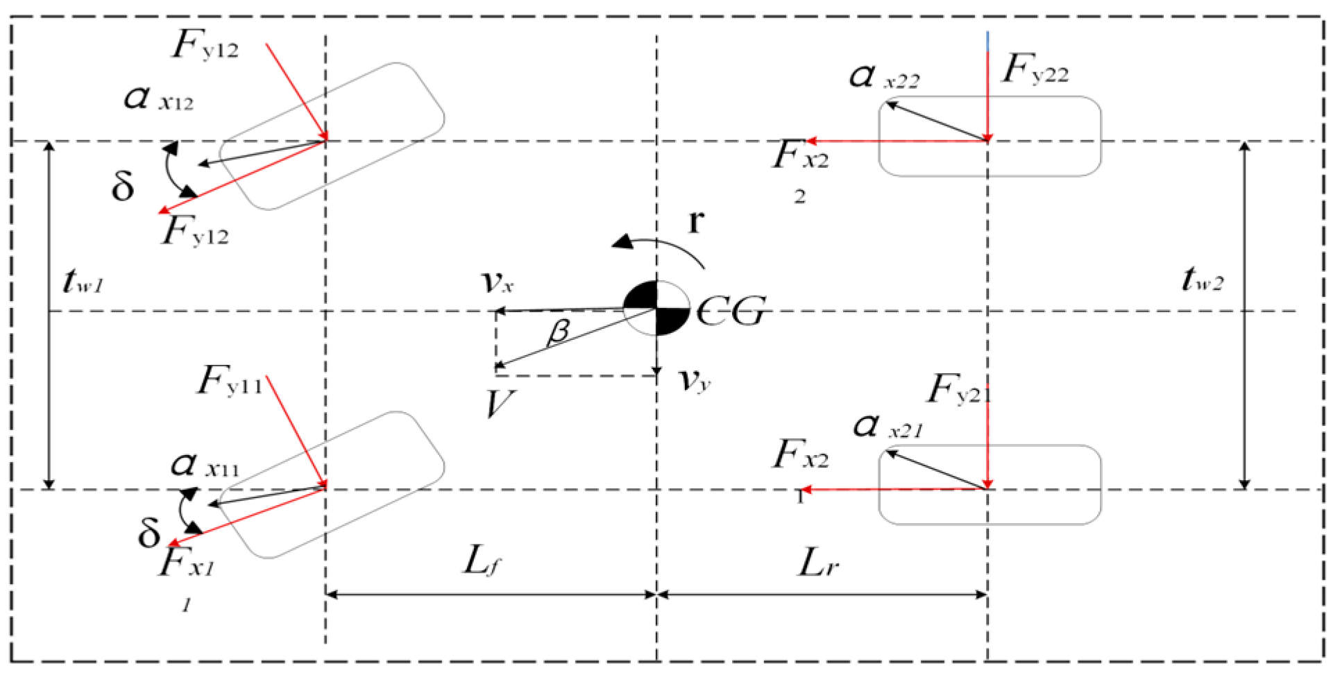
Accurately acquiring dynamic state parameters during vehicle operation is fundamental for controlling vehicle dynamics. Nevertheless, while a vehicle is in motion, it behaves as a highly complex system that is not linear. The conventional two-degrees-of-freedom model (2-DOF), which assumes linearity, cannot adequately represent the vehicle’s nonlinear state. This study proposes a nonlinear 3-DOF vehicle model. Figure 1 is the 3-DOF model and makes the following assumptions:
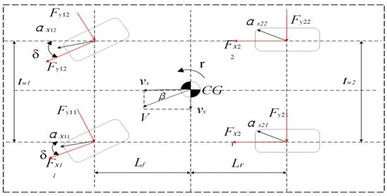
Figure 1.
The 3-DOF model represents the dynamics of a vehicle.
- (1)
- The vehicle’s center of gravity is located at the origin of the coordinate system and possesses structural symmetry;
- (2)
- The degrees of freedom in pitch, roll, and vertical directions are disregarded, along with the influences of air resistance and slope resistance;
- (3)
- The steering system’s impact is disregarded, with the front wheel angle selected as the system’s input;
- (4)
- The body is rigidly connected to the chassis, with the role of the vehicle suspension neglected;
- (5)
- The vehicle’s mass distribution is assumed to be uniform and constant without considering mass transfer during acceleration or deceleration.
Below are the equations for the 3-DOF vehicle dynamics:
where and indicate the longitudinal and lateral forces the tires exert, respectively (). , and represent the track width of the front and rear wheels, respectively., represent the longitudinal and lateral speeds at the center of mass of the vehicle, respectively. denotes the vehicle’s curb weight. and denote the front and rear axle distances to the center of mass, respectively. denotes the steering angle of the front wheels.
2.2. Tire Model
Instead of relying on theoretical frameworks, tire semi-empirical models incorporate realistic data and provide advantages such as streamlined calculations, enhanced real-time performance, and increased accuracy [32]. The Magic Formula and Dugoff tire models are among the most commonly used. Given the need for real-time computation and computational efficiency, this study utilizes the Dugoff tire model. The following calculation formula is obtained by disregarding the camber angle and concentrating just on the tire’s longitudinal and lateral forces:
where stands for the road adhesion coefficient. The boundary condition U is used to determine the current state of each tire and represents the wheel center velocity. indicates the lateral stiffness of the tire. indicates the longitudinal stiffness of the tire. represents the longitudinal slip coefficient of the vehicle. determines the tire slip angle.
The formula for calculating the wheel center velocity for each wheel is as follows:
where , respectively, represent the wheelbases of the front and rear wheels of the vehicle.
By replacing the calculated wheel center velocity for each wheel, it is possible to determine the longitudinal slip ratio for each wheel.
The slip angle of the tires can be determined using the following formulas.
3. Design of Vehicle State Estimator Based on IMM-MCCKF
The CKF assumes that noise follows a Gaussian distribution and demonstrates robust estimation performance in environments with Gaussian noise. However, in practical vehicular environments, noise frequently exhibits non-Gaussian characteristics, leading to diminished performance of the CKF. The MCC is a statistical analysis and signal processing strategy that is highly effective in dealing with noise that has non-Gaussian distributions. Based on the concept of correntropy, it estimates signals by optimizing a nonlinear cost function, thereby enhancing the capability to capture and process signals with heavy tails or outliers. Consequently, integrating the MCC with the CKF enhances the latter’s ability to suppress non-Gaussian noise. In a single MCCKF filter, the noise matrix remains constant, hindering timely and accurate responses to changes in the system model, which can result in estimation errors. The IMM theory facilitates the parallel operation of multiple submodels, each with distinct noise characteristics, thereby mitigating the impact of statistical noise uncertainty. Therefore, this study proposes the IMM-MCCKF algorithm.
3.1. Vehicle State-Space Model
Based on Equations (1)–(3), the vehicle’s longitudinal, lateral, and yaw dynamics are formulated as recursive discrete state equations, as illustrated below:
where represents the state vector and represents the measurement vector. The system noise is characterized by its covariance array . The measurement noise is defined by its covariance array .
The vehicle’s state and measurement models, derived from discretizing Equations (1)–(3) with the first-order Euler method, are expressed as follows:
3.2. Derivation of the Maximum Correntropy Criterion
Based on a specified joint distribution function , the correntropy criteria quantify the degree of resemblance involving two independent variables and . The following is a mathematical definition of the idea of correntropy:
where refers to a translation-invariant kernel that satisfies Mercer’s theorem and represents the expectation operator. The Gaussian kernel is a commonly selected kernel function in correntropy applications.
where represents the correntropy’s kernel bandwidth.
Due to the restricted size of samples used in real-world applications, the joint distribution function is typically unknown. Consequently, the associated entropy is customarily approximated as follows:
where , let be the N samples drawn from .
The Taylor series is used to enlarge the Gaussian kernel, as shown below:
The related entropy is a calculated value determined by adding together all of the even-order error variables, with the weighting of each variable being influenced by the kernel bandwidth parameter.
With MCC, the goal function can be expressed in the following way when dealing with inaccurate data :
3.3. Derivation of the Cubature Kalman Filter Algorithm
The CKF is particularly well suited for state estimation in high-dimensional systems. The complete algorithm for the CKF is as follows [32]:
3.3.1. Predict
Determine the cubature points following the propagation of the nonlinear state equation.
The forecast state is calculated using Equation (25).
Determine the predicted error covariance matrix using Equation (26).
3.3.2. Update
The cubature points are calculated using Equation (27).
The propagated cubature points of the nonlinear state equation are calculated using Equation (28).
The measured state is estimated using Equation (29).
The innovation error covariance matrix is estimated using Equation (30).
The cross-covariance matrix is estimated using Equation (31).
The Kalman gain, updated state, and the error covariance matrix are estimated using Equations (32)–(34).
3.4. Derivation of the MCCKF
Against non-Gaussian noise, correlation entropy performs very well as a suppressor. Due to the noise-sensitive characteristics of the CKF filtering algorithm, combining MCC and CKF facilitates the derivation of the MCCKF algorithm.
Regarding the nonlinear system represented by Equation (13), the nonlinear recursive model is constructed in conjunction with Equation (25), as outlined below:
where
The following is a representation of the covariance.
Multiplying Equation (36) from the left yields the solution to Equation (36).
where , .
Subsequently, using MCC as a basis, define the cost function:
where the jth row of is represented by , and is the most effective solution obtained by substituting the relevant variables into the equation.
Then, this results in the following equation:
where the anticipated state error and the measurement error are quadratically weighted using the covariance matrix , and are defined as follows:
where the components of vector a are used to construct the diagonal matrix . Since is nonlinear, it can be further expanded at the current estimate as follows:
where and are variables corresponding to the fixed-point algorithm at t − 1. Defining , the following results can be derived.
By applying the matrix inversion theorem, Equation (44) can be rewritten as follows:
where .
From which it can be derived that
The covariance is represented by Equation (52).
3.5. Derivation of the IMM-MCCKF Algorithm
The IMM algorithm features adaptive adjustments that enable real-time probability modifications for each submodel. Using the probability transition matrix, the output invariably favors the submodel with the minimum error [33]. Although the MCCKF can effectively suppress non-Gaussian heavy-tailed noise, a fixed-noise matrix reduces estimation accuracy when the system model undergoes sudden noise changes. Consequently, this paper integrates the IMM with MCCKF to develop the IMM-MCCKF algorithm, addressing the decreased accuracy in MCCKF during sudden model noise fluctuations. Each submodel employs identical state and measurement vectors, with the MCCKF employed to construct the filters, thereby minimizing the impact of uncertainty from prior noise statistical data. The specific derivation process is outlined below:
where represents the Markov probability transition matrix.
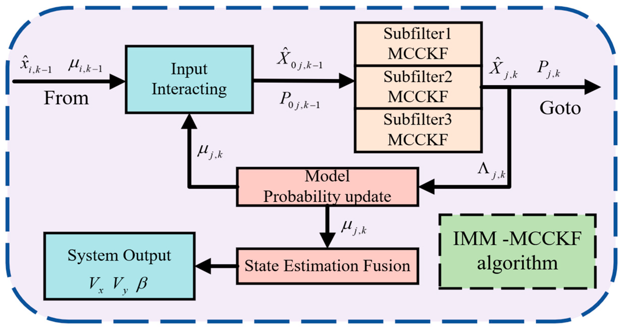
Figure 2 shows the iterative process of the IMM-MCCKF.

Figure 2.
IMM-MCCKF algorithm’s iterative process.
3.5.1. Interaction Input
represents the state estimation results of each filter from the previous time step. Similarly, describes the model probabilities of each filter of the prior time step. The state estimation value and covariance are calculated based on and .
The obtained estimation values are set as the initial values for the IMM algorithm. The computation method proceeds as detailed below [7]:
where .
3.5.2. Model Filtering
Based on the MCCKF iteration process, and covariance from the interaction is substituted into the jth model, resulting in the estimation value , covariance matrix , measurement output , and corresponding covariance matrix after model filtering.
- Update of the probability model.
The probability distribution function of the jth model:
Model j’s probability:
- 2.
- Output interaction:
The derivation of the IMM-MCCKF is completed as outlined above, with the pseudocode for the IMM-MCCKF presented in Algorithm 1.
| Algorithm 1: IMM-MCCKF Pseudocode. |
| For i = 1: N |
| 1 Input: , |
| 2 Interaction |
| Using Equation (54) to calculate |
| Using Equations (55) and (56) to initialize |
| 3 Model Filtering |
| Using Equations (25) and (26) to calculate |
| Using Equations (29) and (31) to calculate |
| Using Cholesky decomposition to calculate |
| Let and repeat |
| Using Equations (49) and (50) to calculate |
| Using Equations (45)–(48) to calculate |
| if , |
| Using Equation (52) to calculate |
| 4 Model Probability Update |
| Using Equations (57)–(59) to calculate |
| Using Equations (60) and (61) to calculate |
| Using Equations (62) and (63) to calculate |
| 5 Output: |
| end |
4. Simulation Verification
4.1. Configuration of Simulation Experiment Environment
A collaborative simulation was conducted using MATLAB/Simulink and the vehicle simulation program CarSim to assess the efficacy and accuracy of the IMM-MCCKF technique in estimating vehicle state parameters. Starting with a C-class car model from CarSim, building an electric vehicle model with distributed drive. Additionally, a drive motor model was constructed using MATLAB/Simulink. The simulation sampling time was configured to 0.001 s, which allowed for the input of sensor signals necessary for estimating the vehicle’s state in Simulink. Furthermore, non-Gaussian noise was introduced into the sensor input signals to assess the algorithm’s estimation performance under non-Gaussian noise conditions. Table 1 contains the whole set of parameters for the C-class vehicle model, and Figure 3 shows the procedure of the estimate algorithm.

Table 1.
The simulation parameter table for a C-class vehicle in CarSim.

Figure 3.
IMM-MCCKF workflow diagram.
An IMM-MCCKF vehicle state parameter estimator was developed in MATLAB/Simulink and designed to test two vehicle operating scenarios: double lane-change and sinusoidal steering. While maintaining consistent input parameters, the MCCKF and CKF algorithms were compared in simulation experiments.
The Markov transition matrix in this paper is configured according to Equation (64):
During the actual operation of the vehicle, sensor measurements can be affected by outliers, rendering sensor noise typically non-Gaussian. This paper models the sensor signals that occur during the operation of a vehicle. The system’s process and measurement noise assumes a non-Gaussian distribution with heavy tails. The model adheres to the specified covariance matrix criteria.
Considering the uncertainty in process and measurement noise during actual vehicle operation, different noise levels are empirically assigned to the submodels of the IMM-MCCKF algorithm as follows:
where 1, 2, and 3 represent submodel 1, submodel 2, and submodel 3, respectively.
Both submodels have process and measurement noise that is ten and a hundred times higher than the original model. This paper compares the MCCKF and CKF algorithms using noise parameters that align with submodel 1 of the IMM-MCCKF. The system state and measurement equations are also consistent with the IMM-MCCKF.
4.2. Experimental Results and Analysis
This study presents the results of simulation investigations using sinusoidal steering and double-lane-changing scenarios. Under these scenarios, the system’s driving state undergoes significant changes, thus effectively demonstrating the effectiveness of the method proposed in this paper.
4.2.1. Double-Lane-Change Scenario
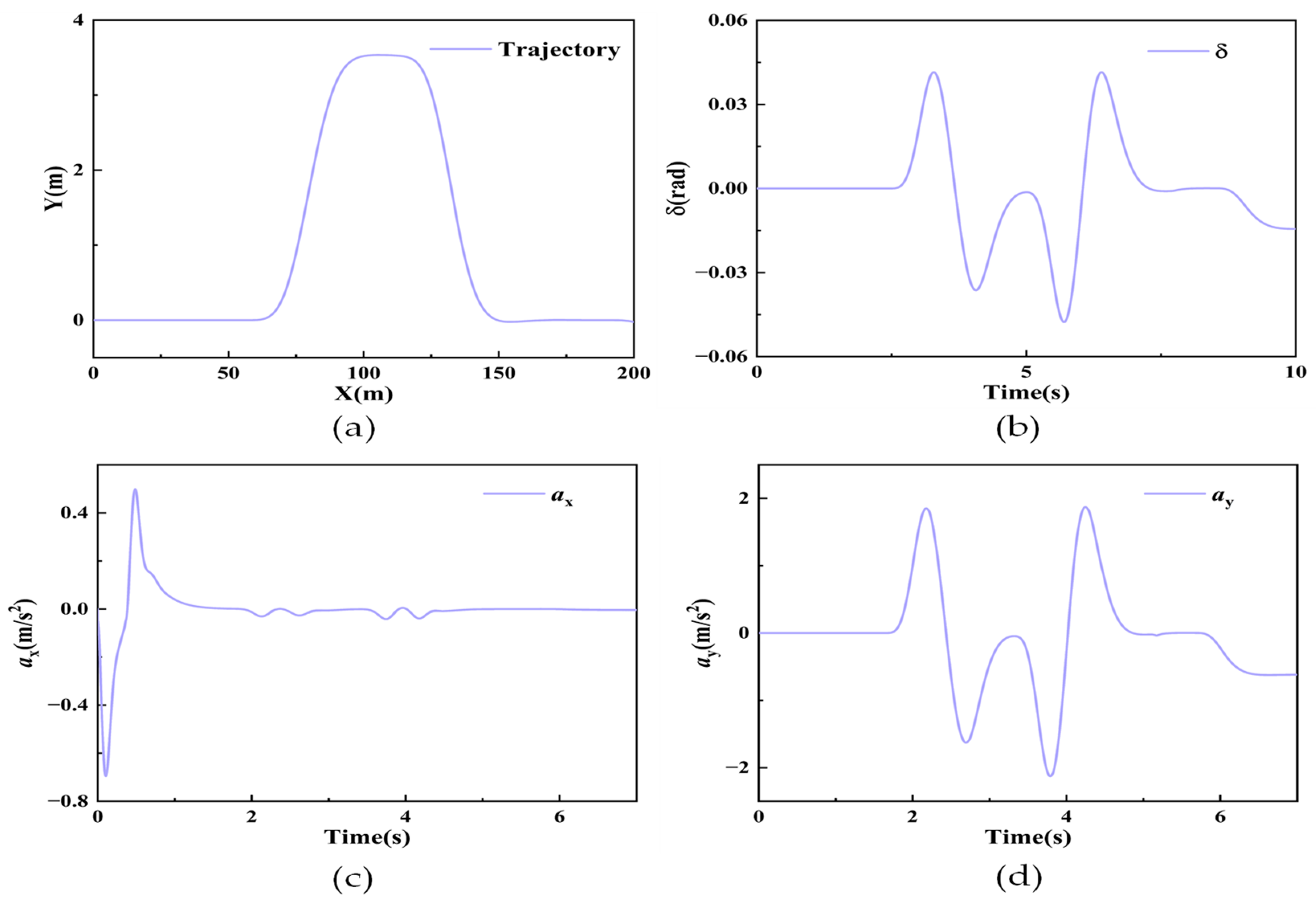
Using the corresponding covariance matrix from Equation (66) and the road adhesion coefficient of 0.85, assuming that the measurement noise and process are non-normally distributed. , are the system’s initial state parameters. Figure 4 shows the input signals. Figure 5 shows the simulation results.
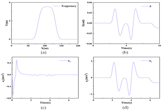
Figure 4.
Input signals for the double-lane-change scenario: (a) the vehicle trajectory, (b) the angle of the front wheels, (c) the longitudinal acceleration, and (d) the vertical acceleration.
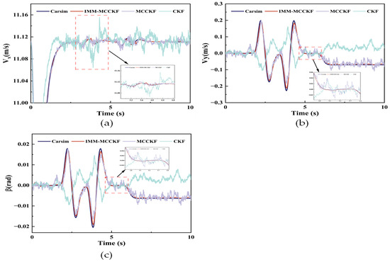
Figure 5.
Simulation results for the double-lane-change scenario: (a) longitudinal velocity, (b) lateral velocity, and (c) centroid sideslip angle.
Figure 5 displays the outcomes of the vehicle’s simulated double-lane-change scenario. It can be observed from Figure 5a that both IMM-MCCKF and MCCKF maintain high accuracy in longitudinal speed estimation, and their performance is superior to that of CKF. However, compared to MCCKF, the estimates from IMM-MCCKF are more accurate, reducing the impact of individual outlier errors.
According to Figure 5b,c, the IMM-MCCKF algorithm also ensures high accuracy under extreme conditions, with smoother estimation curves demonstrating better robustness. Due to the limited ability of MCCKF and CKF to resist noise variations, their estimation curves show some fluctuations, with CKF’s results exhibiting significant oscillations and divergence trends. According to the Dugoff tire model, the tires enter a nonlinear operating zone when the vehicle’s steering angle approaches extreme conditions, increasing tire forces. Additionally, the increase in outlier data from onboard sensors enhances the non-Gaussian nature of the noise, resulting in more significant estimation errors in CKF.
4.2.2. Sinusoidal Steering Scenario
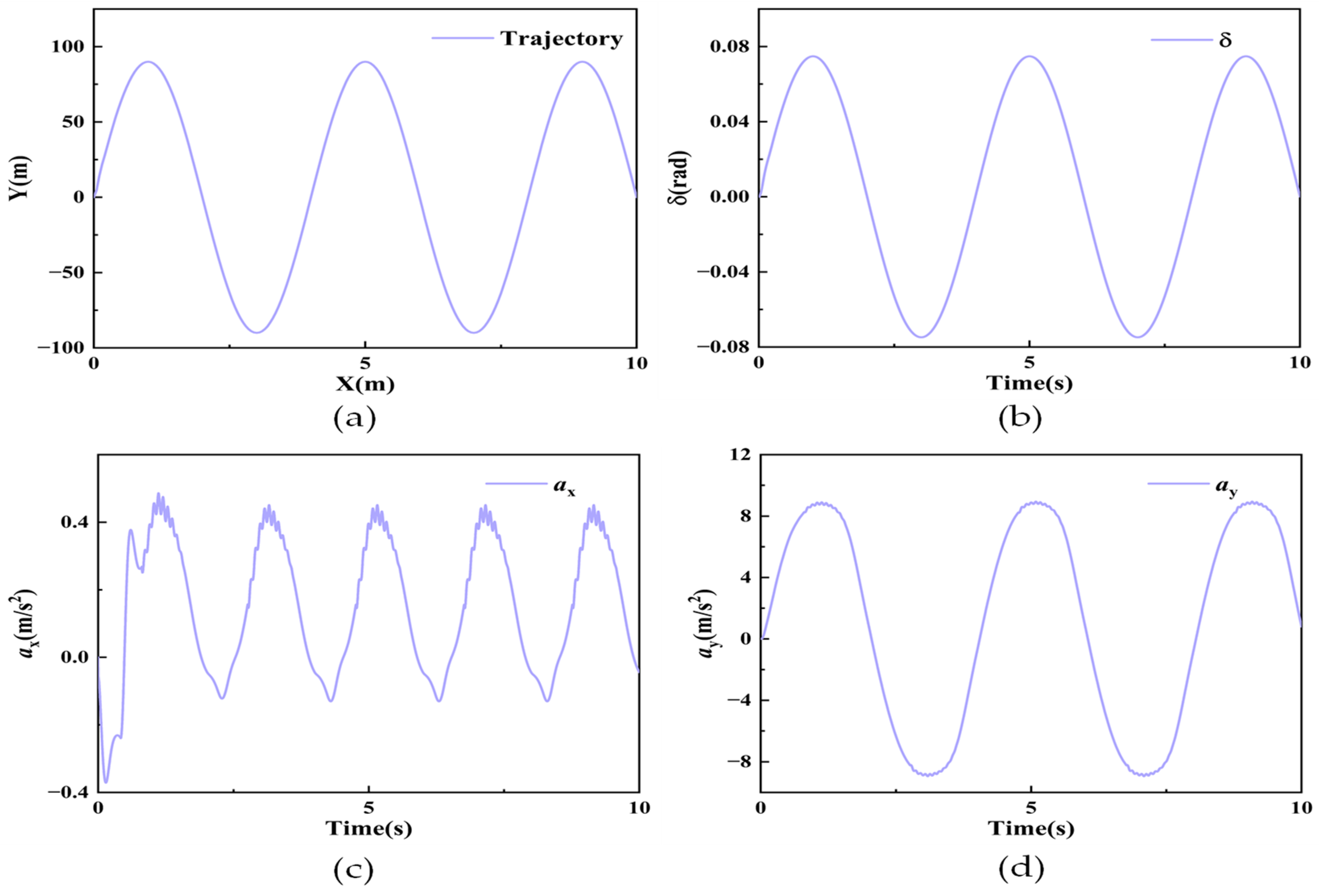
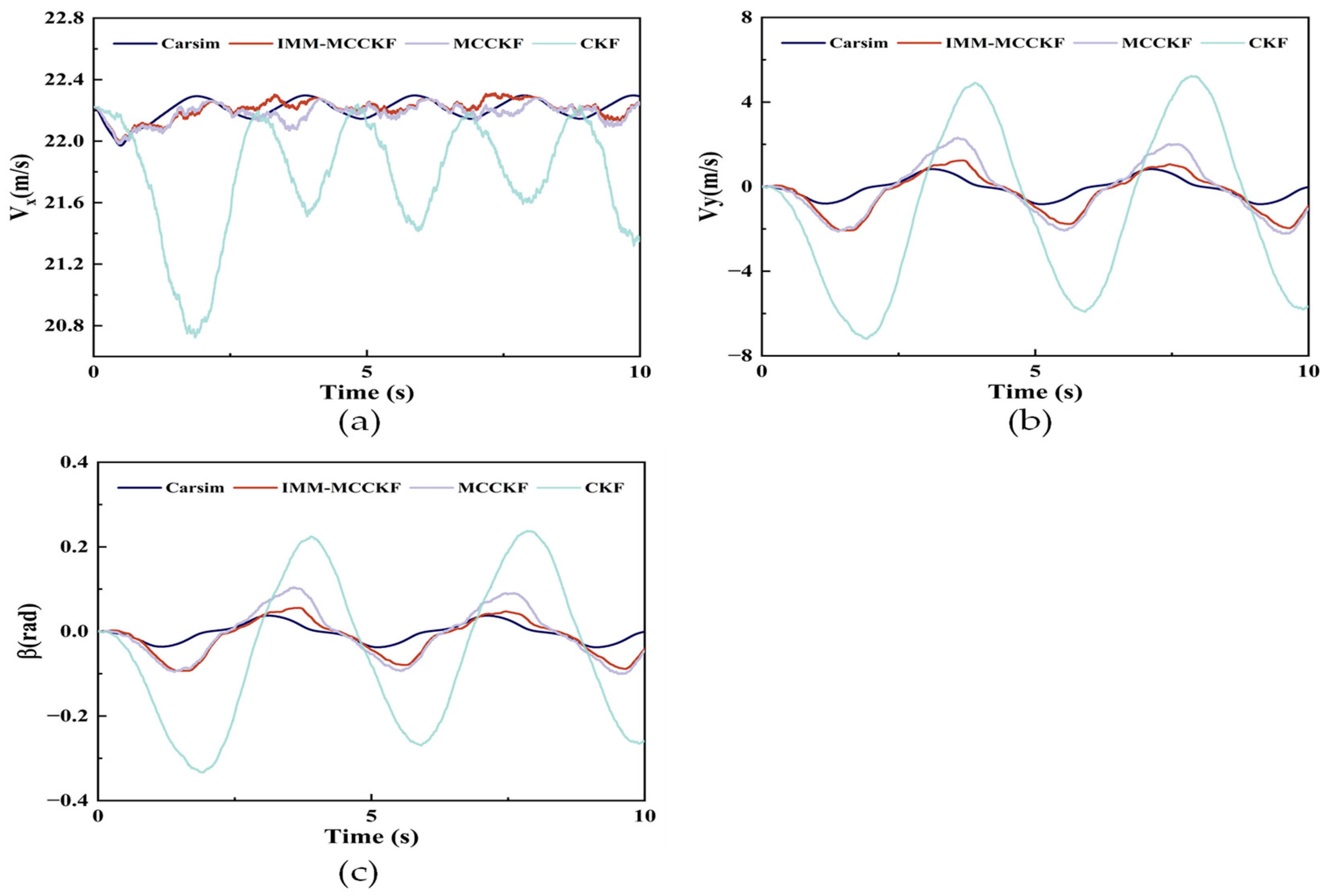
The sinusoidal steering scenario was set for further validation to verify the algorithm’s effectiveness under extreme high-speed conditions. The system’s initial state parameters are specified as , . Currently, the road adhesion coefficient is kept at 0.85, and the vehicle is set to maintain a constant speed of 80 km/h. Figure 6 presents the driving trajectory of the estimator, along with the input and observation signals. Figure 7 compares simulation results between the IMM-MCCKF and the MCCKF and CKF algorithms.
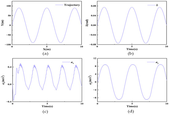
Figure 6.
Input signals for the sinusoidal steering scenario: (a) the vehicle trajectory, (b) the angle of the front wheels, (c) the longitudinal acceleration, and (d) the vertical acceleration.
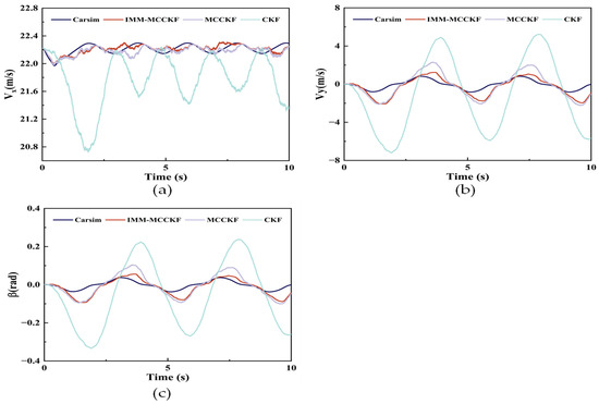
Figure 7.
Simulation results for the sinusoidal steering scenario: (a) longitudinal velocity, (b) lateral velocity, and (c) centroid sideslip angle.
Figure 7 presents the simulation outcomes for the vehicle’s sinusoidal steering scenario, with Figure 7a–c displaying longitudinal speed, lateral speed, and the centroid sideslip angle, respectively. As illustrated in Figure 7a, both IMM-MCCKF and MCCKF accurately track the actual value in longitudinal speed estimation, while CKF exhibits significant fluctuations and deviations in its estimates. All three algorithms exhibit estimation errors when the vehicle enters a nonlinear zone while cornering at high speeds, as illustrated in Figure 7b,c. This difference is due to the lateral force being calculated slightly differently from the actual value.
Due to the vehicle’s pronounced nonlinear characteristics during high-speed continuous cornering and the susceptibility of sensor data to outliers, the non-Gaussian nature of the noise is enhanced, resulting in more significant estimation errors at peak points. Consequently, CKF produces inaccurate estimates when non-Gaussian noise is present, and its performance drops dramatically. Although MCCKF has good noise suppression capabilities, its ability to resist noise variations is weak, resulting in decreased estimation performance. Conversely, IMM-MCCKF can quickly adjust model probabilities and maintain model outputs with more minor errors, thereby ensuring high estimation accuracy and superior tracking performance. In summary, the IMM-MCCKF algorithm continuously monitors the model with a minor mistake through a Markov probability transition matrix by adjusting model probabilities in real time based on each submodel process and observation.
5. Comparative Analysis and Discussion
Equation (67) defines RMSE, used in a quantitative analysis to compare the three algorithms’ estimation performance under two conditions. The results are as shown in Table 2.
Table 2.
Analyzing RMSE values in two different simulation scenarios.
Table 2 shows that compared to the MCCKF and CKF algorithms the IMM-MCCKF algorithm has significantly lower RMSE values in the double-lane-change and sinusoidal steering scenarios. The IMM-MCCKF algorithm integrates IMM and MCCKF, allowing it to adapt to different noise environments dynamically and more effectively suppress non-Gaussian noise.
In the double-lane-change scenario, the IMM-MCCKF algorithm reduces the RMSE in longitudinal speed by approximately 15.3% compared to MCCKF and 68.6% compared to CKF. The reduction in RMSE for lateral speed is even more significant, with decreases of 67.0% and 94.8%, respectively. The IMM-MCCKF algorithm makes real-time adjustments to the model’s probabilities, aligning the output with the model with the fewest errors. In contrast, the CKF algorithm exhibits significant fluctuations and divergence.
The IMM-MCCKF algorithm also demonstrates excellent estimation performance in the sinusoidal steering scenario. It reduces the RMSE in longitudinal speed by 16.5% compared to MCCKF and by 89.6% compared to CKF. The RMSE is reduced by 32.1% and 82.5% for lateral speed, respectively.
In summary, CKF performs well in Gaussian noise environments but poorly under non-Gaussian noise conditions, resulting in significant estimation errors. MCCKF, which combines the MCC with CKF, better handles non-Gaussian noise; however, a single MCCKF filter has limitations in dynamically adapting to noise variations, leading to decreased estimation accuracy when noise changes suddenly. By incorporating IMM theory into MCCKF, the IMM-MCCKF algorithm overcomes the limitations of CKF and MCCKF. IMM-MCCKF can dynamically adapt to noise variations by integrating multiple submodels with different characteristics, maintaining estimation accuracy and stability under non-Gaussian noise conditions.
6. Conclusions
This study proposes an IMM-MCCKF filter for vehicle state parameter estimation and compares the performance of the IMM-MCCKF, MCCKF, and CKF filters. Simulation experiments were conducted under low-speed double lane-change and high-speed sinusoidal steering scenarios. In the double-lane-change condition, CKF showed significantly decreased estimation performance, whereas IMM-MCCKF and MCCKF maintained high accuracy. According to Table 2, the IMM-MCCKF algorithm reduced errors in longitudinal and lateral speed estimation by 15.3% and 67.0%, respectively, compared to MCCKF. Under the sinusoidal steering scenario, the CKF algorithm exhibited significant estimation fluctuations and a diverging trend. Both IMM-MCCKF and MCCKF maintained high accuracy and stability in their estimates.
The IMM-MCCKF uses the MCC to optimize a nonlinear cost function, effectively suppressing non-Gaussian noise and capturing and processing outlier data in signals. Furthermore, it incorporates various state and measurement noise submodels that dynamically adapt to environmental changes, thereby mitigating the impact of unknown noise statistical properties. The study conducted simulation tests under two different driving scenarios: double lane-change and sinusoidal steering. The obtained results were contrasted and analyzed quantitatively using RMSE. The results demonstrate that the IMM-MCCKF filter, as proposed in this study, delivers superior estimation performance under heavy-tailed non-Gaussian noise conditions compared to the MCCKF and CKF algorithms. Additionally, under extreme conditions, IMM-MCCKF effectively counters the interference of noise variations, maintaining minimal fluctuations in the estimation results, thereby providing accurate vehicle state parameters essential for implementing autonomous driving systems and active safety in intelligent vehicles.
In future work, more sophisticated vehicle models will be applied to parameter estimation modeling, and the algorithms detailed in this study will be validated using public datasets.
Author Contributions
Conceptualization, Q.C., F.Z. and L.S.; methodology, Q.C. and F.Z.; software, L.S. and B.L.; validation, F.Z., S.C. and Y.Z.; formal analysis, Q.C.; investigation, L.S., B.L. and S.C.; resources, Q.C., F.Z. and Y.Z.; data curation, Q.C. and F.Z.; writing—original draft preparation, Q.C.; writing—review and editing, Q.C., F.Z. and L.S.; visualization, Q.C. and B.L.; supervision, F.Z. and S.C.; project administration, F.Z. and L.S.; funding acquisition, F.Z. and B.L. All authors have read and agreed to the published version of the manuscript.
Funding
This research was supported by the National Key Research and Development Program of China (2021YFB2500704).
Institutional Review Board Statement
Not applicable.
Informed Consent Statement
Not applicable.
Data Availability Statement
The original contributions presented in the study are included in the article, further inquiries can be directed to the corresponding author.
Acknowledgments
The authors thank the editors and the anonymous reviewers for their valuable remarks and recommendations.
Conflicts of Interest
Authors Liang Su and Baoxing Lin were employed by the company King Long United Automotive Industry. The remaining authors declare that the research was conducted in the absence of any commercial or financial relationships that could be construed as a potential conflict of interest.
Abbreviations
| CKF | Cubature Kalman filter |
| EKF | Extended Kalman filter |
| MCC | Maximum correntropy criterion |
| MCCKF | Maximum correntropy criterion Kalman filter |
| UKF | Unscented Kalman filter |
| Tire longitudinal force | |
| Tire lateral force | |
| Track width | |
| Curb weight | |
| Longitudinal speeds | |
| Lateral speeds | |
| Longitudinal slip ratio | |
| Front wheel angle | |
| Road adhesion coefficient | |
| Wheel center velocity | |
| Tire stiffness | |
| Tire slip angle | |
| Wheelbase | |
| The state vector | |
| The measurement vector | |
| Correntropy | |
| Kernel function | |
| Weight factor | |
| Process noise covariance matrix | |
| Measurement noise covariance matrix | |
| Error term | |
| Weight matrix | |
| Observation matrix | |
| Kernel function | |
| Normalization factor | |
| Transition probability | |
| Threshold | |
| kernel bandwidth |
References
- Zhang, H.; Guo, J.; Luo, G.; Li, L.; Na, X.; Wang, X.; Teng, S.; Ma, S.; Li, Y. Emerging Trends in Intelligent Vehicles: The IEEE TIV Perspective. IEEE Trans. Intell. Veh. 2023, 8, 3983–3995. [Google Scholar] [CrossRef]
- Zhang, Z.; Zheng, L.; Li, L.; Wu, X.; Yu, Y. Research on Intelligent Vehicle Target State Tracking Based on Robust Adaptive SCKF. J. Mech. Eng. 2021, 57, 181. [Google Scholar] [CrossRef]
- Yao, Q.; Tian, Y.; Wang, Q.; Wang, S. Control Strategies on Path Tracking for Autonomous Vehicle: State of the Art and Future Challenges. IEEE Access 2020, 8, 161211–161222. [Google Scholar] [CrossRef]
- Marcano, M.; Diaz, S.; Perez, J.; Irigoyen, E. A Review of Shared Control for Automated Vehicles: Theory and Applications. IEEE Trans. Hum.-Mach. Syst. 2020, 50, 475–491. [Google Scholar] [CrossRef]
- Chen, L.; Li, Y.; Huang, C.; Li, B.; Xing, Y.; Tian, D.; Li, L.; Hu, Z.; Na, X.; Li, Z.; et al. Milestones in Autonomous Driving and Intelligent Vehicles: Survey of Surveys. IEEE Trans. Intell. Veh. 2023, 8, 1046–1056. [Google Scholar] [CrossRef]
- Xia, X.; Hashemi, E.; Xiong, L.; Khajepour, A. Autonomous Vehicle Kinematics and Dynamics Synthesis for Sideslip Angle Estimation Based on Consensus Kalman Filter. IEEE Trans. Control Syst. Technol. 2023, 31, 179–192. [Google Scholar] [CrossRef]
- Wan, W.; Feng, J.; Song, B.; Li, X. Vehicle State Estimation Using Interacting Multiple Model Based on Square Root Cubature Kalman Filter. Appl. Sci. 2021, 11, 10772. [Google Scholar] [CrossRef]
- Song, R.; Fang, Y. Vehicle State Estimation for INS/GPS Aided by Sensors Fusion and SCKF-Based Algorithm. Mech. Syst. Signal Process. 2021, 150, 107315. [Google Scholar] [CrossRef]
- Welch, G.; Bishop, G. An Introduction to the Kalman Filter; Department of Computer Science, University of North Carolina at Chapel Hill: Chapel Hill, NC, USA, 1995. [Google Scholar]
- Wang, X.; Wang, A.; Wang, D.; Xiong, Y.; Liang, B.; Qi, Y. A Modified Sage-Husa Adaptive Kalman Filter for State Estimation of Electric Vehicle Servo Control System. Energy Rep. 2022, 8, 20–27. [Google Scholar] [CrossRef]
- Wang, Y.; Xu, L.; Zhang, F.; Dong, H.; Liu, Y.; Yin, G. An Adaptive Fault-Tolerant EKF for Vehicle State Estimation with Partial Missing Measurements. IEEE/ASME Trans. Mechatron. 2021, 26, 1318–1327. [Google Scholar] [CrossRef]
- Julier, S.J.; Uhlmann, J.K. New Extension of the Kalman Filter to Nonlinear Systems. Signal Process. Sens. Fusion Target Recognit. VI 1997, 3068, 182–193. [Google Scholar]
- Zhang, Y.; Li, M.; Zhang, Y.; Hu, Z.; Sun, Q.; Lu, B. An Enhanced Adaptive Unscented Kalman Filter for Vehicle State Estimation. IEEE Trans. Instrum. Meas. 2022, 71, 6502412. [Google Scholar] [CrossRef]
- Katriniok, A.; Abel, D. Adaptive EKF-Based Vehicle State Estimation with Online Assessment of Local Observability. IEEE Trans. Control Syst. Technol. 2016, 24, 1368–1381. [Google Scholar] [CrossRef]
- Arasaratnam, I.; Haykin, S. Cubature Kalman Filters. IEEE Trans. Autom. Control 2009, 54, 1254–1269. [Google Scholar] [CrossRef]
- Wang, Y.; Zhang, F.; Geng, K.; Zhuang, W.; Dong, H.; Yin, G. Estimation of Vehicle State Using Robust Cubature Kalman Filter. In Proceedings of the 2020 IEEE/ASME International Conference on Advanced Intelligent Mechatronics (AIM), Boston, MA, USA, 6–9 July 2020; pp. 1024–1029. [Google Scholar]
- Benzerrouk, H.; Nebylov, A.; Salhi, H. Quadrotor UAV State Estimation Based on High-Degree Cubature Kalman Filter. IFAC-PapersOnLine 2016, 49, 349–354. [Google Scholar] [CrossRef]
- Kim, J.H.; Yoon, S.W. Dual Deep Neural Network Based Adaptive Filter for Estimating Absolute Longitudinal Speed of Vehicles. IEEE Access 2020, 8, 214616–214624. [Google Scholar] [CrossRef]
- Khalid, H.M.; Flitti, F.; Muyeen, S.M.; Elmoursi, M.; Sweidan, T.; Yu, X. Parameter Estimation of Vehicle Batteries in V2G Systems: An Exogenous Function-Based Approach. IEEE Trans. Ind. Electron. 2022, 69, 9535–9546. [Google Scholar] [CrossRef]
- Chen, J.; Cheng, L.; Gan, M.-G. Extension of SGMF Using Gaussian Sum Approximation for Nonlinear/Non-Gaussian Model and Its Application in Multipath Estimation. Acta Autom. Sin. 2013, 39, 1–10. [Google Scholar] [CrossRef]
- Pryseley, A.; Tchonlafi, C.; Verbeke, G.; Molenberghs, G. Estimating Negative Variance Components from Gaussian and Non-Gaussian Data: A Mixed Models Approach. Comput. Stat. Data Anal. 2011, 55, 1071–1085. [Google Scholar] [CrossRef]
- Mohseni, H.R.; Kringelbach, M.L.; Woolrich, M.W.; Baker, A.; Aziz, T.Z.; Probert-Smith, P. Non-Gaussian Probabilistic MEG Source Localisation Based on Kernel Density Estimation. NeuroImage 2014, 87, 444–464. [Google Scholar] [CrossRef]
- Wang, G.; Xue, R.; Wang, J. A Distributed Maximum Correntropy Kalman Filter. Signal Process. 2019, 160, 247–251. [Google Scholar] [CrossRef]
- Liu, X.; Chen, B.; Xu, B.; Wu, Z.; Honeine, P. Maximum Correntropy Unscented Filter. Int. J. Syst. Sci. 2017, 48, 1607–1615. [Google Scholar] [CrossRef]
- Shao, J.; Chen, W.; Zhang, Y.; Yu, F.; Chang, J. Adaptive Multikernel Size-Based Maximum Correntropy Cubature Kalman Filter for the Robust State Estimation. IEEE Sens. J. 2022, 22, 19835–19844. [Google Scholar] [CrossRef]
- Ge, P.; Zhang, C.; Zhang, T.; Guo, L.; Xiang, Q. Maximum Correntropy Square-Root Cubature Kalman Filter with State Estimation for Distributed Drive Electric Vehicles. Appl. Sci. 2023, 13, 8762. [Google Scholar] [CrossRef]
- Fakoorian, S.; Santamaria-Navarro, A.; Lopez, B.T.; Simon, D.; Agha-mohammadi, A. Towards Robust State Estimation by Boosting the Maximum Correntropy Criterion Kalman Filter with Adaptive Behaviors. IEEE Robot. Autom. Lett. 2021, 6, 5469–5476. [Google Scholar] [CrossRef]
- Xu, Y.; Zhang, W.; Tang, W.; Liu, C.; Yang, R.; He, L.; Wang, Y. Estimation of Vehicle State Based on IMM-AUKF. Symmetry 2022, 14, 222. [Google Scholar] [CrossRef]
- Ndjeng Ndjeng, A.; Gruyer, D.; Glaser, S.; Lambert, A. Low Cost IMU–Odometer–GPS Ego Localization for Unusual Maneuvers. Inf. Fusion 2011, 12, 264–274. [Google Scholar] [CrossRef]
- Jo, K.; Chu, K.; Sunwoo, M. Interacting Multiple Model Filter-Based Sensor Fusion of GPS With In-Vehicle Sensors for Real-Time Vehicle Positioning. IEEE Trans. Intell. Transp. Syst. 2012, 13, 329–343. [Google Scholar] [CrossRef]
- Choi, J.W.; Samuel, K. Robust UKF-IMM Filter for Tracking an Off-Road Ground Target. Int. J. Control Autom. Syst. 2019, 17, 1149–1157. [Google Scholar] [CrossRef]
- Xin, X.; Chen, J.; Zou, J. Vehicle State Estimation Using Cubature Kalman Filter. In Proceedings of the 2014 IEEE 17th International Conference on Computational Science and Engineering, Chengdu, China, 19–21 December 2014; pp. 44–48. [Google Scholar]
- Li, R.; Jilkov, V.P. Survey of Maneuvering Target Tracking. Part v: Multiple-Model Methods. IEEE Trans. Aerosp. Electron. Syst. 2005, 41, 1255–1321. [Google Scholar] [CrossRef]


Disclaimer/Publisher’s Note: The statements, opinions and data contained in all publications are solely those of the individual author(s) and contributor(s) and not of MDPI and/or the editor(s). MDPI and/or the editor(s) disclaim responsibility for any injury to people or property resulting from any ideas, methods, instructions or products referred to in the content. |
© 2024 by the authors. Licensee MDPI, Basel, Switzerland. This article is an open access article distributed under the terms and conditions of the Creative Commons Attribution (CC BY) license (https://creativecommons.org/licenses/by/4.0/).