Abstract
Depth map estimation is crucial for a wide range of applications. Unfortunately, it often presents missing or unreliable data. The objective of depth completion is to fill in the “holes” in a depth map by propagating the depth information using guidance from other sources of information, such as color. Nowadays, classical image processing methods have been outperformed by deep learning techniques. Nevertheless, these approaches require a significantly large number of images and enormous computing power for training. This fact limits their usability and makes them not the best solution in some resource-constrained environments. Therefore, this paper investigates three simple hybrid models for depth completion. We explore a hybrid pipeline that combines a very efficient and powerful interpolator (infinity Laplacian or AMLE) and a series of convolutional stages. The contributions of this article are (i) the use a Texture+Structuredecomposition as a pre-filter stage; (ii) an objective evaluation with three different approaches using KITTI and NYU_V2 data sets; (iii) the use of an anisotropic metric as a mechanism to improve interpolation; and iv) the inclusion of an ablation test. The main conclusions of this work are that using an anisotropic metric improves model performance, and the ablation test demonstrates that the model’s final stage is a critical component in the pipeline; its suppression leads to an approximate 4% increase in . We also show that our model outperforms state-of-the-art alternatives with similar levels of complexity.
1. Introduction
Depth data have become a key source of information for a wide variety of applications, such as robotics and augmented reality. Notably, a depth map is an image whose pixels represent the distance from the object’s surface to a fixed point in the scene (typically a sensor capturing the data). There are many sensors to acquire depth data, including structured light and RealSense sensors, ToF (Time-of-Flight) cameras, LiDAR (Light Detection and Ranging), and stereo vision. Regardless of the sensor type, depth data are characterized by low quality in terms of missing data, noise, and errors. Missing data are particularly dramatic, since in some cases the depth maps present large areas with no information or “holes”. Completing depth information in those cases becomes an extremely challenging interpolation problem.
Hence, we can define the depth completion problem as the problem of interpolating or filling in the missing gaps in a depth image. It was originally tackled using classical interpolation techniques in image processing and later using more sophisticated inpainting methods. These last methods performed well in simple scenarios at high computational costs. Unfortunately, they presented limitations in more complex real-world situations. For that reason, researchers explored other approaches, such as bilateral filtering and non-local means filtering, which leverage local image features and image statistics to propagate depth information across empty regions. These models achieved significant improvement but still performed poorly in some real-world situations, for instance, in the presence of large holes corresponding to portions of the reference (color) image without significant texture. It was not until the arrival of deep learning that depth completion experienced a breakthrough, leading to high-quality maps. Nevertheless, despite the success of deep learning algorithms, classical approaches remain relevant in some applications, mainly due to their explainability, computational efficiency, and ability to operate on resource-constrained platforms.
In this work, we explore a non-deep-learning approach that provides good-quality depth maps in constrained environments. We propose a simple and flexible model that requires few images for training and can, consequently, run on a laptop with only one GPU; thus, it represents a low-cost implementation alternative. This paper extends the work presented at the 14th International Workshop on Parallel and Distributed Algorithms and Applications, PDAA [1]. The contributions of this manuscript are as follows:
- 1.
- We employ a balanced metric, which considers a balance term between spatial and photo-chromatic distance.
- 2.
- We evaluate the impact of an additional Texture+Structure decomposition stage.
- 3.
- We propose two variations of the previous interpolation model.
- 4.
- We apply an ablation test to our model in the NYU_V2 data set.
1.1. Examples of Incomplete Depth Maps
Here, we illustrate some examples of incomplete depth maps (Figure 1) caused either by sensor misinterpretations, estimation errors, or other factors. Some of these errors may be due to occlusions, transparency, or reflections, among other reasons.
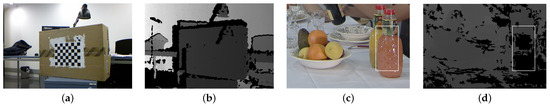
Figure 1.
Examples of depth maps containing large areas of missing data. (a) Reference color image. (b) Depth map, holes (in black) due to occlusions. (c) Color reference image; a white square indicates reflections. (d) Depth map with holes in areas of high reflection due to uncertainty in the stereo-matching process.
1.2. Organization of This Manuscript
In the next section, we present a brief state of the art and discuss relevant approaches in the field. Next, Section 3 presents our approach, including the underlying mathematical model and the data set employed for training and evaluation. Section 4 details the process for estimating the model parameters. Section 5 presents the performance evaluation. Finally, the conclusion is stated in Section 6.
2. State of the Art
Many image interpolation-related problems have used a scene’s color information to guide the propagation of some other type of information, such as depth inpainting and image enhancement [2]. Depth completion is not an exception. Similarly, the geometry of color images has been used to drive a diffusion process completing sparse depth maps [3]. A bilateral filter is one of the most classic examples of a guided method. This image-domain filter considers regional color characteristics, such as edges and smooth areas, to slow or accelerate depth propagation, respectively.
More recently, deep learning techniques have taken the lead. For instance, Lu et al. [4] proposed completing a sparse depth image jointly by reconstructing a gray-level scene image, using convolutional neural networks. They evaluated this method using the KITTI [5] data set, which is a publicly available data set and one of the most popular databases for performance evaluation in the field. Another deep learning approach by Yang et al. [6,7] utilizes a CNN-based model to interpolate depth data from a Kinect sensor database.
Another example is the work of Imran et al. [8]. Their proposal focused on preventing the generation of mixed-depth pixels, that is, pixels that are neither background nor foreground, which are typical in object discontinuities. They proposed a new and interesting representation of pixels called Depth Coefficients (DCs). Hence, the loss function used to train the network is based on the DC representation, leading to a depth interpolation that tries to make more accurate decisions on the image edges. Zhang et al. [9] additionally proposed a model to complete depth maps based on an RGB image and a sparse depth map. Using the RGB image and a deep neural network, the authors estimated the normals of the surfaces in the scene. Using this information and the raw depth data acquired by a sensor, the authors minimized a depth estimation error for the whole image. They evaluated their proposal using their own data set. The results show that it outperforms classical models such as TGV [10] and bilateral filters.
In the work of [11], the authors proposed a model to complete depth data. Their proposal used a unified CNN framework incorporating two features: (a) a model considering the relation between normals and surfaces in the depth value, and (b) a model predicting the confidence of the depth data. In this way, this model predicts surface normals, depth, and depth confidence values simultaneously. These estimations are inputs for a refinement module in order to obtain the final depth estimation. Evaluations of the model in the KITTI and NYU_V2 data sets show that the model presents state-of-the-art performance.
The work in [12] presents a non-local depth completion model, which is different from other non-local models because the proposal dynamically selects more informative neighbors. The depth completion is iteratively refined using confidence values assigned to the depth data. The model also incorporates learned affinity to improve the accuracy of depth estimation, avoiding the “mixed depth” in the edges of the objects in the scene. Experiments show that the proposal outperforms DeepLidar and FuseNet [13] in the KITTI data set.
In [14], a CNN model that fuses sparse depth data and color information to complete a depth map is presented. The model uses two approaches: one processes the color image, and the second refines the depth completion. The outputs from both approaches are combined in order to improve the depth completion. Furthermore, the 3D information of the scene is used to improve the depth estimation. The model achieves state-of-the-art performance in the KITTI data set, outperforming contemporary models.
Lin et al. [15] proposed a model using Dynamic Spatial Propagation Networks. This type of network dynamically estimates the parameters of an affinity. The authors proposed a diffusion suppression procedure to stop diffusion close to the edges of the color image. The most relevant feature of this model is its rapid convergence compared to models with similar architectures.
The paper in [16] presents a deep learning model for depth completion that creates content-dependent and spatially variant kernels. The authors proposed a new convolutional factorization to store the large amount of data associated with these kernels’ parameters. This new factorization reduces the computational cost of the model. The proposed model outperforms others in the NYU_V2 and KITTI data sets.
Nevertheless, one of the most well-known limitations of deep learning depth completion models is their huge number of parameters (requiring millions of parameters). Researchers are aware of this drawback, and some improvements have been explored in this direction, for instance, in the work of Bai et al. [17]. Their proposal can reduce the number of parameters by up to 96% compared to similar approaches. Thanks to that, the authors can deploy their model on an FPGA, achieving real-time performance (interpolating 11.1 images per second).
Although these are relevant advances, there is still a need to develop more computationally efficient (non-deep-learning) solutions capable of providing relatively high-quality depth maps with much less computational effort. In this paper, we follow this direction, presenting a simple interpolator based on the infinite Laplacian. This model has already been successfully applied in other image interpolation problems, such as the interpolation of optical flow on video in Lazcano et al. [3].
The origins of this interpolator trace back to the foundational work of Caselles et al. [18]. The authors applied an axiomatic approach to data interpolation, stating a set of properties that a well-behaved interpolator should hold. One of the interpolators holding the full set of axioms was the infinity Laplacian.
More recently, Lazcano et al. [19] also proposed a practical implementation of the infinity Laplacian and the biased infinity Laplacian models. One of the most relevant contributions was the proposal of a Euclidean metric that included a spatial and a color term. The infinity Laplacian provided the best results for upsampling images in the context of the Middlebury data set.
In addition to the infinity Laplacian, there is a panoply of computationally efficient techniques in the literature. For instance, in [20], the authors segmented the reference color image using superpixels and the SLIC algorithm. A 2D linear interpolation approach was used to generate a depth-value plane using the depth information in each superpixel. The model incorporated heuristics and simple rules to tackle depth estimation when segmentation errors occurred. The results outperformed the bilateral filtering approach.
A more recent and interesting approach is the work by Saidi et al. [21]. The authors proposed a real-time algorithm capable of estimating up to 111 depth maps per second. Unfortunately, the estimated depth maps presented missing or low-confidence data.
Table 1 summarizes the number of parameters, GPUs, and images in the training set reported in the literature of cited methods.

Table 1.
Model training comparison table.
Table 1 shows that most models use thousands of images for training and more than one GPU, and two report thousands of parameters to be estimated.
Last but not least, it is important to mention that some consensus has been reached by the depth completion community regarding performance evaluation. Researchers used well-established data sets, which include clear evaluation protocols, to benchmark their solutions. This article will use two popular data sets: KITTI [5] and NYU_V2 [25].
3. Materials and Methods
In this section, we present the use of the infinity Laplacian, or AMLE (Absolutely Minimizing Lipschitz Extension), for the interpolation of sparse depth maps. We selected the infinity Laplacian because it is (i) simple to solve, (ii) fast to compute, and (iii) easy to implement. As we will explain in Section 3.7, the infinity Laplacian has several parameters, requiring a small training set to estimate them.
We embedded the infinity Laplacian in a pipeline, considering convolutional stages to enforce features or filter noise. In the following subsections, we explain the interpolation model and the pipeline.
3.1. Depth Interpolation Models
We used the infinity Laplacian to interpolate or complete the available depth data. The infinity Laplacian model was initially proposed by Aronsson in the 1960s, and it is the simplest interpolator that satisfies a set of axioms [18]. We will explain the infinity Laplacian in Section 3.7.
3.2. Pipeline
Figure 2 shows the proposed pipeline to complete depth maps. The input to the pipeline is a CIE-Lab reference image. The pipeline includes a feature-extraction convolutional stage, an interpolation stage, and a noise-removal convolutional stage.
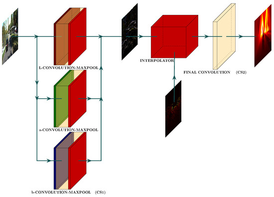
Figure 2.
Proposed pipeline structure. It consists of three steps. CS1 extracts color features from the reference image using Gabor filters. Then, the algorithm propagates the acquired available depth data, with the guidance of the color image, to all regions of the sparse depth map by solving the infinity Laplacian equation (interpolator). Finally, we use a convolution stage (CS2) to eliminate outliers and noise from the completed depth map.
3.2.1. Convolutional Stage (CS1)
We processed each color component (L, a, b) of the reference image with a certain number of Gabor filters, (), to extract the color features. The Gabor filters and their parameters are as follows:
where
, is the rotation angle, and is the spatial frequency.
Then, we max-pooled the output of the filters in each color component and normalized the output to the range 0–255. Finally, we concatenated the normalized color components to create a color feature image. Figure 3 shows some examples of processed images.
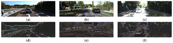
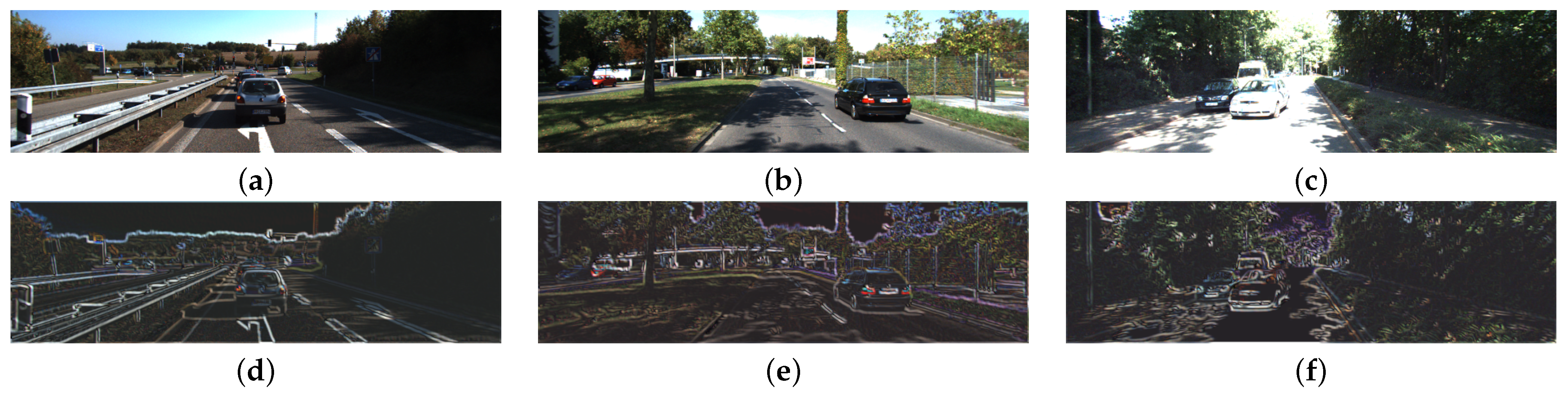
Figure 3.
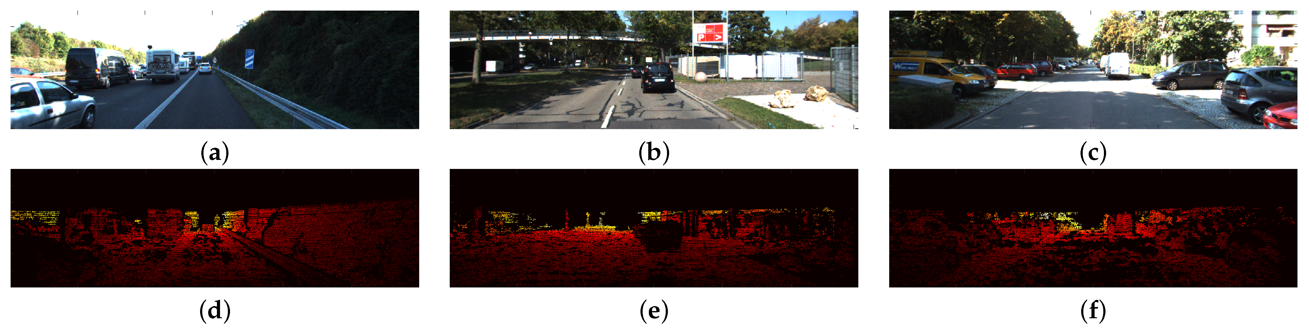
Examples of color reference images processed by the first convolutional stage. Figures (a–c) show the color reference image extracted from the KITTI data set. In (d–f), we present their respective output after being processed by the first convolutional stage (color feature images). We observe in (d–f) that the processing mainly emphasizes horizontal edges in order to improve the diffusion process.
For the examples shown, the first stage enforces horizontal edges due to the characteristics of the images. These images were acquired by a horizontal laser scan using a LiDAR sensor, which is why the horizontal edges were particularly relevant to drive diffusion.
The parameters used for each one of the Gabor filters were estimated through a training process. We will detail this process in Section 4.
3.2.2. Interpolator (Infinity Laplacian)
As shown in Figure 2, the central element of the proposal is the infinity Laplacian interpolator. The infinity Laplacian takes two inputs: a color reference image and a sparse depth map. The model interpolates the available depth data, guided by the color reference image. This interpolation is achieved by solving the degenerated second-order partial differential equation, the infinity Laplacian, using the available depth data. The solution of the infinity Laplacian propagates the available data to the empty regions. This propagation is performed through a diffusion process based on an anisotropic metric, which is explained in Section 3.7.
3.3. Final Convolutional Stage (CS2)
In this stage, we process the output of the infinity Laplacian by a bank of average filters, eliminating noise and outliers. The eight parameters of the filters are estimated in the training stage (see Section 4).
3.4. Pipeline with a Variable Structure
The proposed pipeline can dynamically change the order in which the stages process the images (processing sequence). As mentioned earlier, the order depicted in Figure 2 is CS1–Interpolator–CS2, but depending on a boolean parameter, the processing sequence can be CS2–Interpolator–CS1. The dimensions and number of filters in each stage are adjusted to allow the processing sequence to be inverted. The idea behind this operation is that the structure of the model switches during training. Once the parameters of the model are determined, they are set into the pipeline, and after that, the model is used to process the validation set.
3.5. Variable Number of Filters
The Gabor and average filters in our proposal are variable, ranging from 1 to 8 and 1 to 9, respectively. Only two parameters define the number of used filters ( and ). These parameters are estimated during the training and set after that.
3.6. Texture+Structure Decomposition
An image can be decomposed into its structural () and textural () components using the Rudin–Osher–Fatemi (ROF) total variation denoising model. The structural component is obtained by solving for the intensity values of the image :
where is the original image, its domain, and . We remark that .
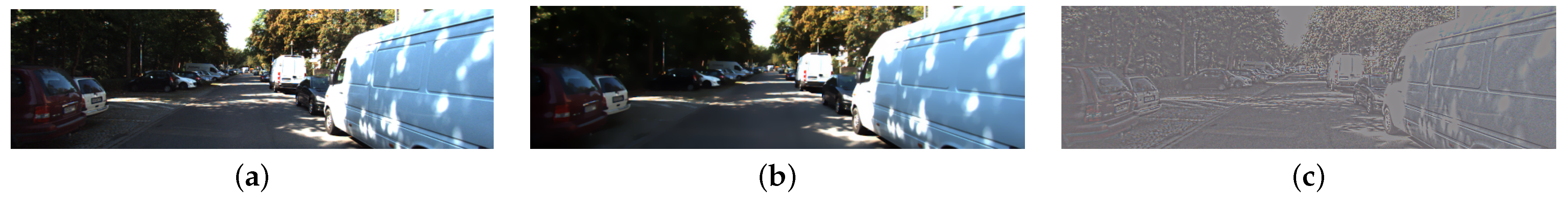
We used the Texture+Structure decomposition to pre-process the color reference image. This way, the texture components (high spatial variations) and the structure of the image (low spatial variations) were extracted from the reference image. Figure 4 shows an example of the Texture+Structure decomposition.

Figure 4.
Example of Texture+Structure decomposition. (a) Original color reference image. (b) Low spatial variation part of the image. (c) High spatial variation part of the image (texture component).
3.7. Infinity Laplacian
The interpolator used to complete the sparse depth maps is the infinity Laplacian, or AMLEhows. The infinity Laplacian is the simplest model that holds a set of axioms for interpolators [18]. Suppose is the image domain. For each incomplete depth map u, we solve the following problem:
where is the infinity Laplacian, g is the metric, and u is the interpolated depth data. Let us consider the image domain as a rectangle, let be a domain in a smooth compact two-dimensional manifold embedded in . The interpolated surface u, or manifold, is obtained by solving the infinity Laplacian, Equation (4), in the domain. Considering solving the infinity Laplacian in this 2D surface , the infinity Laplacian is stated as
which is a degenerated elliptic PDE. Let us consider the depth map u as , and the available data are located in , i.e., . Considering the boundary condition for the infinity Laplacian, we set the available depth data to a constant value on the domain’s boundary. This fact ensures that the completed depth map agrees with the available data at the boundary.
As a proof of concept, we will show an example of data interpolation using the infinity Laplacian. Figure 5 shows a simple example of depth completion using the infinity Laplacian.
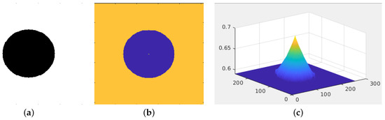
Figure 5.
Example of depth completion by the infinite Laplacian. We show the reference image in (a). The image consists of a white rectangle, and in its center, there is a black circle. We show the depth data in (b). The orange region represents a constant depth of 0.5; in the center, the circle in blue represents the lack of data. In the center of the blue circle, there is only a single value equal to 0.68. We show the interpolated depth map in (c). The infinity Laplacian generates a cone, connecting the circular contour with the point in the circle’s center.
Figure 5 shows a depth map in (a) with a circular hole to be completed. Furthermore, the circle has a unique depth data point in its center. Let be the coordinates of the depth data point in the center of the circle, and let be the circular contour of radius 60 centered at . Then, we state that and . We solve the infinity Laplacian in Equation (4), obtaining the cone shown in Figure 5c.
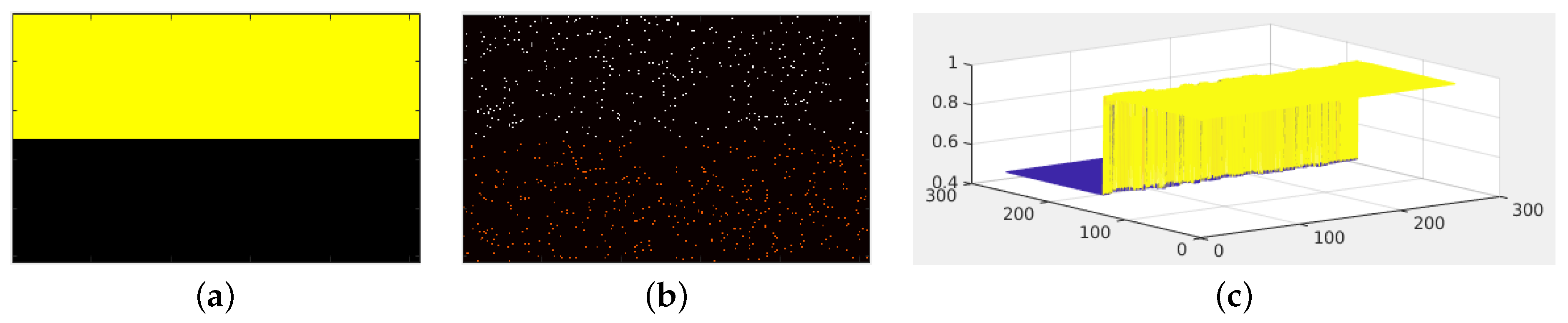
In Figure 6, we show a second simple example where we complete a two-level depth image given random depth samples.
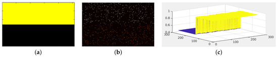
Figure 6.
Example of depth map completion. (a) shows a two-color reference image. (b) shows random samples of a two-level depth map. White values represent the value 1, and orange values represent the depth value 0.5. Figure (c) shows a 3D representation of the completed depth map. We observe the two-level surface.
Figure 6a shows the reference color image of this second toy example. Figure 6b shows the sampled depth map. We sampled 2% of the depth data image, which is around 1300 samples. The completed two-level depth data are plotted in 3D in Figure 6c.
Equation (4) was discovered by Aronsson in the nineteen-sixties as an Euler–Lagrange equation for the problem of the Absolutely Minimizing Lipschitz Extension (or AMLE):
where u is the extension of the available data. Computing the Euler–Lagrange equation of Equation (6), we have
that is to say,
and when , we have
where is the Laplacian of u computed in the gradient direction.
The infinity Laplacian model enables the creation of cones and soft surfaces, which could be more suitable for completing urban scenes.
3.8. Variations in the Infinity Laplacian
The biased infinity Laplacian is a variation of the original in Equation (9) used in [19]. This operator additionally considers the modulus of the gradient of u:
where the c parameter is a positive real value. For the value , we recover the infinity Laplacian. We state variations in the biased infinity Laplacian, namely the balanced biased infinity Laplacian adding a balance term :
The balance term can be explicitly computed as
where and are real positive parameters that will be estimated in the training stage. is a balanced map ; depending on the necessity of the completion process, the model balances between infinity Laplacian and the eikonal operator. A second variation of this proposal is called the double balanced infinity Laplacian, which considers the infinity Laplacian using the eikonal operators in Equation (11):
where is a similar mechanism to , defined as
with and . We remark that if , we recover the biased infinity Laplacian.
3.9. Metric
Let us consider the reference color image as a function from the domain to the color space, i.e., , and the metric , conforming to the manifold . Considering , we solve Equation (4). We explored different metrics to estimate the shape of the manifold in order to better approximate the geodesic distance. In a preliminary work [19], we tested the following metric:
where the constants and are estimated in the training stage. This metric comprises two terms: a spatial distance term and a photo-chromatic distance term . The first term is the spatial distance of pixels and in the image domain . The second term is the photo-chromatic distance in the CIE-Lab color space between and . To give more flexibility to this metric, we relaxed the exponents as follows:
where p, q, . We also estimated the exponent values in the training stage.
We stated (in our work presented in [1]) the following metric:
where A and C are positive definite matrices, and is called the positive definite metric.
In this work, we propose an anisotropic metric, which considers a balance term between spatial distance and photo-chromatic distance,
where is defined by
where is the spatial distance, is the photo-chromatic distance, and . On the one hand, if , the difference between should be large, and positive. It means that should be also large, and finally should be small, i.e., . The metric is more confident in the photo-chromatic term.
On the other hand, if , the difference between should be negative. It means that should be small, , that is to say, that , meaning that the metric is more confident in the spatial term. As a proof of concept of , we show estimation examples of the balance term considering a color reference image in Figure 7.
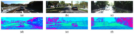
Figure 7.
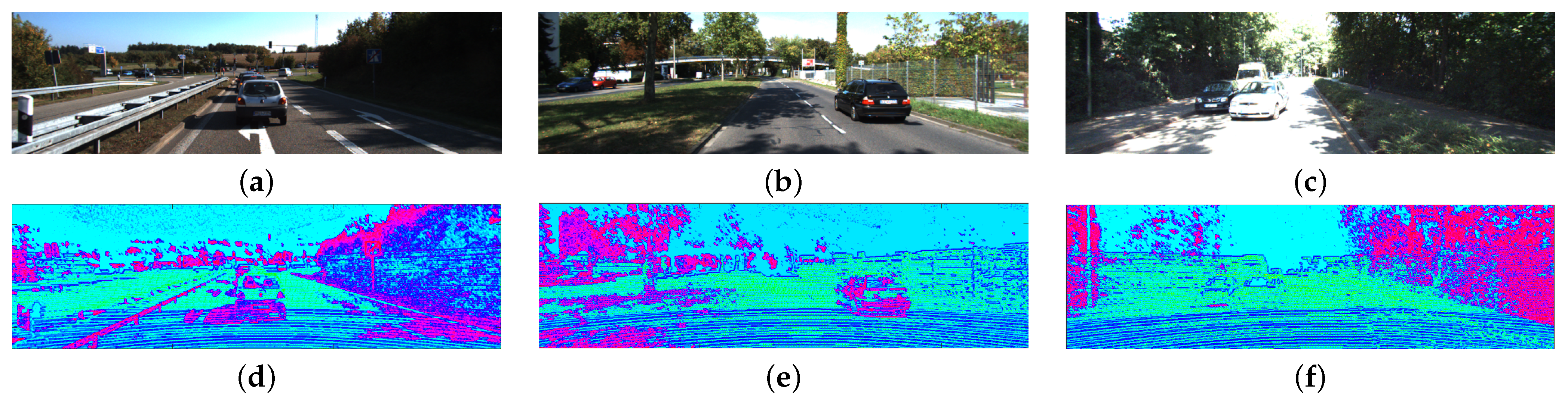
Example of map in three example images. Figures (a–c) show considered reference color images. Figures (d–f) show color-coded values of balance map. In magenta, we show largest values of (). In blue and cyan, we show intermediate values of . In green, we show lowest values of ().
Figure 7 shows color-coded values of the map. Figure 7a–c are reference color images already shown in Figure 3. In Figure 7d–f, we color-coded the values of the map . The metric is more confident in the spatial term in magenta regions. Magenta regions represent objects with shadows and highly textured regions. In blue, we represent , which means that the metric is confident in the spatial term. We can see that the values are less than 0.5 in cyan areas, which is the sky in the reference color image, which means that the metric is confident of both the photo-chromatic and spatial term. In light-green regions, has the smallest values, which means that the metric is more confident in the photo-chromatic term.
3.10. Geodesic Metric Approximation
Let us consider the discrete image domain as a grid, and let and be two points in the grid. We defined a metric in Equation (16) between consecutive points. The geodesic distance between two points in the grid represents the shortest path joining and , i.e.,
that is to say, considering a curve joining and in the grid, the length of is given by
The geodesic distance should be computed using Dijkstra’s algorithm. To increase the efficiency of computing the geodesic distance, we approximated the geodesic distance directly with the following metric:
This approach offers efficient computation while keeping an acceptable level of approximation.
3.11. Solving the AMLE Model
For the sake of completeness, we briefly explain the numerical solution of the infinity Laplacian model as already presented in [26,27]. We remind the reader that the infinity Laplacian is equivalent to
where and are the positive eikonal operator and negative eikonal operator, respectively.
3.12. Practical Model Implementation
Given a point in a neighborhood of , the positive eikonal operator is defined as
and the negative eikonal operator is defined as
Let and be the locations that maximize Equations (20) and (21), respectively. With this definition, it is possible to state the infinity Laplacian,
Solving for ,
The iterated version is
with .
3.13. Numerical Model for the Biased Infinity Laplacian
Taking into account the above definitions (of the biased infinity Laplacian) and substituting in Equation (10), we have
which is a linear equation for ; consequently, we can solve for :
As shown in Equation (26), the solution of the biased infinity Laplacian is only the weighted sum of the and values multiplied by the distance of the center of to the points and , respectively. We remark that
where () is the sign function.
3.14. Numerical Model for the Balanced Biased Infinity Laplacian
Recalling the balanced infinity Laplacian, we substitute it into Equation (11) to obtain
We can solve for :
3.15. Numerical Model for the Double Balanced Biased Infinity Laplacian
Taking into account the above definition and substituting it into Equation (11), we have
Solving for ,
3.16. Iterative Solution of the Infinity Laplacian Variations
3.17. Data Sets
In this work, we use two publicly available data sets, (1) KITTI and (2) NYU_V2, to train and validate the proposed models.
- 1.
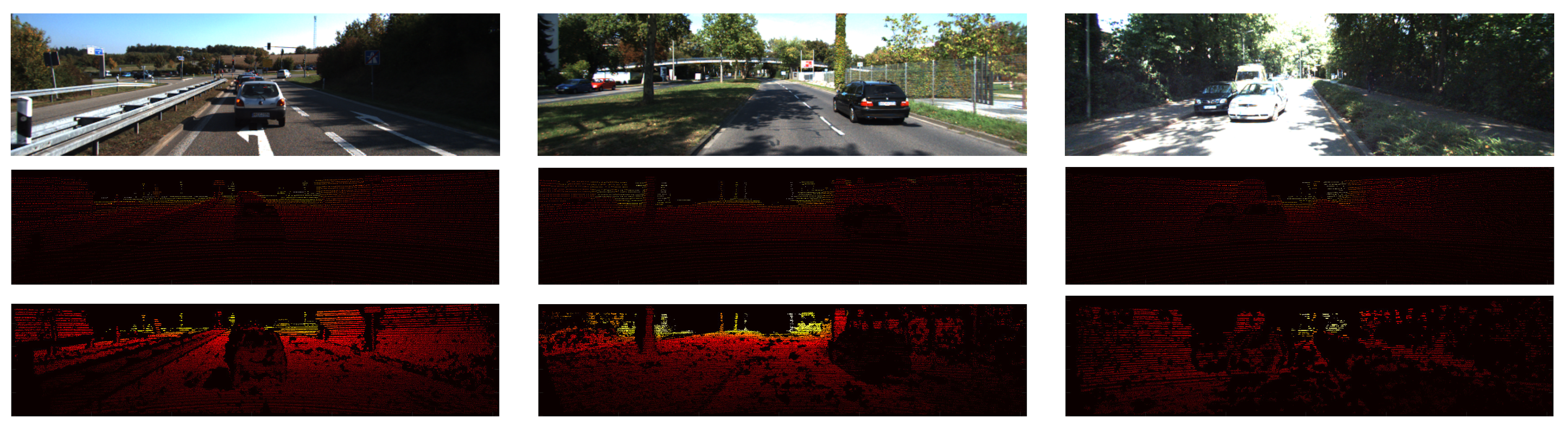
- KITTI depth Completion Suite [5] consists of 1000 color images and depth data of urban scenes acquired by a color camera and a LiDAR (Light Detection and Ranging), respectively, mounted on a vehicle traveling across a city. The vehicle had a color camera on its top, and as the vehicle traveled across the city, its sensors acquired synchronized data. Each color image is accompanied by a corresponding sparse depth map and ground truth, as illustrated in Figure 8.
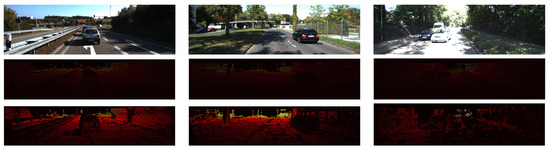 Figure 8. Examples of reference color images of the KITTI data set, sparse depth maps, and ground truth. First row: color reference images. Second row: available sparse depth maps. In the third row, we show the corresponding ground truth. We color-coded the available depth value using a MATLAB jet color map. In the second and third rows, black means a lack of data, and red and yellow mean small and large depth values, respectively.The model was trained using three images extracted from the KITTI data set, with their corresponding depth maps and their corresponding ground truth. We used the 997 remaining images to evaluate the model’s performance.
 - 2.
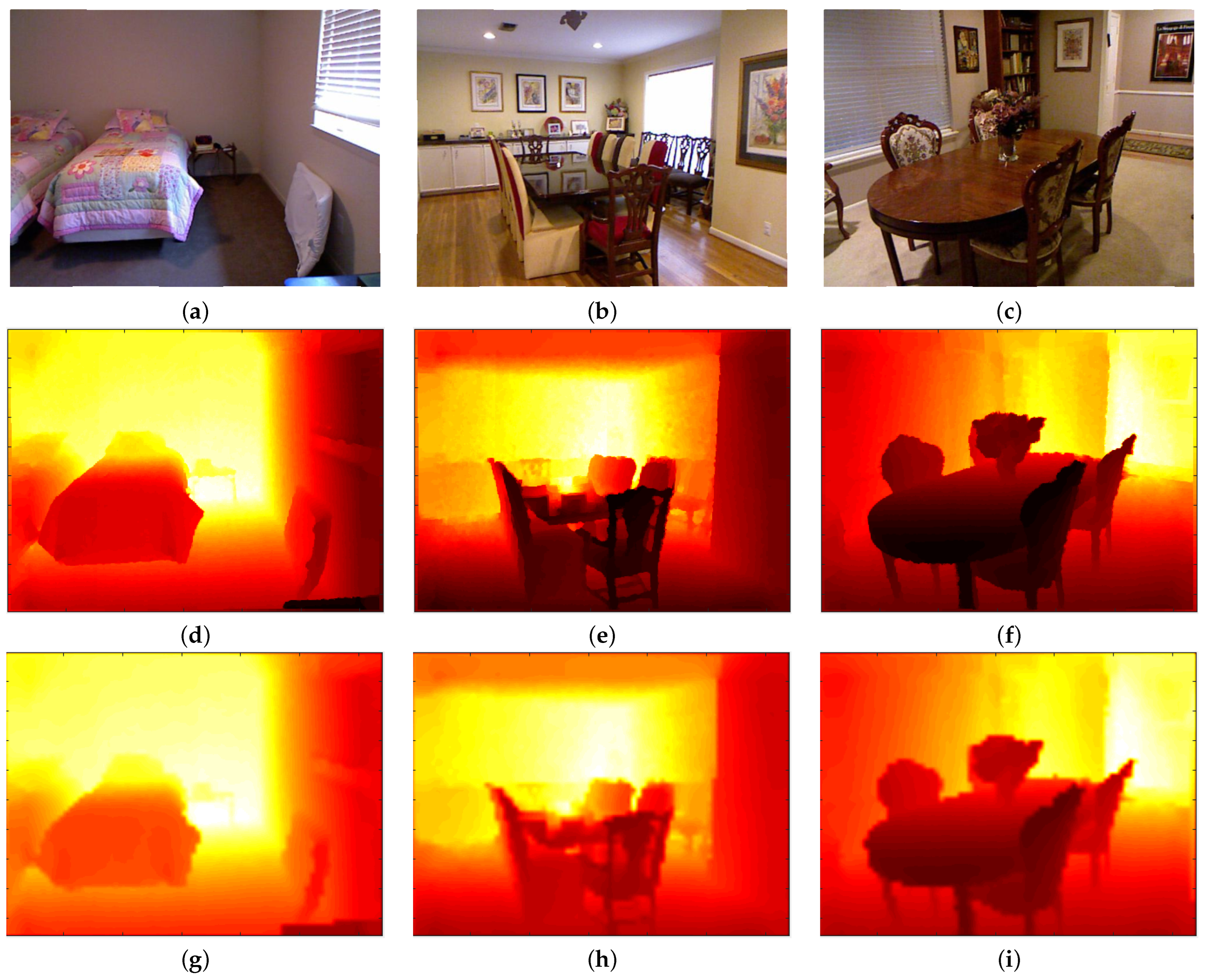
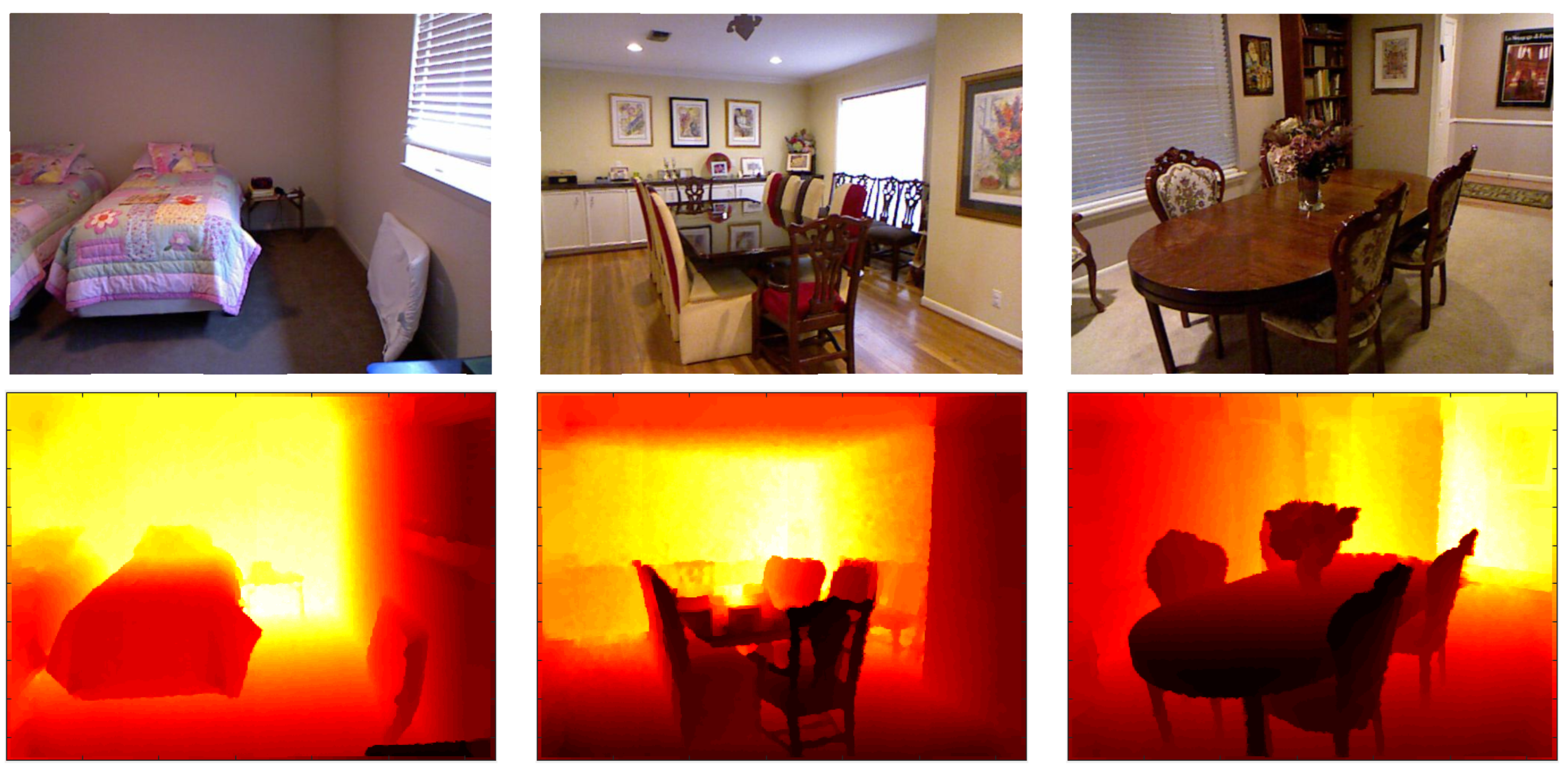
- NYU_V2 data setThe NYU_V2 data set comprises 1449 indoor images and their corresponding depth data acquired by a structure light sensor. In Figure 9, we show some images of NYU_V2.
 Figure 9. Examples of NYU_V2 data set. The first row shows three indoor color images of the NYU_V2 data set. We show images Img_1199, Img_1372, and Img_1424, respectively. We color-coded the corresponding depth map in the second row using MATLAB jet colormap: dark red means small depth values, and bright yellow means large depth values.
 - 3.
- Similarly to the previous data set, three images from NYU_V2 were used to train the model. Images from 1001 to 1449 were used to estimate the model’s performance (as stated in the corresponding protocol).
3.18. Implementation and Complexity
We implemented the proposed model in C++/Cuda and used MATLAB to implement the PSO algorithm and to plot the results. The program runs in Linux 22.04 on a laptop with HP OMEN 16, 16 GB of RAM, a Processor i7-11800H, and an NVIDIA GTX 3070. We measured the processing time. Our computer processed each image with iterations, obtaining a running time of 0.08 ms per iteration. This processing time means that the total processing time is 0.64 ms. Please note that the time to acquire and store the image was not included. Given the above factors, the processing time can be ms.
In terms of complexity, every time we interpolated an image, it was processed pixel-by-pixel. Let N be the number of image pixels, and consider a neighborhood of P pixels around each pixel x. The central pixel is compared with every pixel of the neighborhood, leading to
The size of the neighborhood around x is presented in Table 2:
Table 2.
Number of points per neighborhood size.
For an image of and a logarithm of , if we keep , we have operations.
In Table 3, we report the processing time of our model and other models considered in this paper.
Table 3.
Running time of different models.
Table 3 shows that our model is approximately an order of magnitude faster than the other models.
4. Training the Model
To estimate the model parameters, the PSO (Particle Swarm Optimization) algorithm was applied. In Table 4, we summarize the total number and values of the model parameters:
Table 4.
Parameters of the proposed model.
Each individual in the PSO method is a candidate solution to minimize the Depth Completion Error, given by 50 random instances of (). The error formula is given by
where N is the number of images in the training set, is the Mean square error, and is the Mean absolute error. Given the ground truth, we computed the and errors between the completed depth map and the ground truth of the training set and evaluated the expression (31).
For completeness, we briefly summarize the PSO algorithm, already explained in [1,26]. In each iteration of the algorithm, the candidate solutions evolve based on the dynamical equation for their position and velocity:
and
where , , , and , , and , represent the best current individual and the best individual of all iterations, respectively. Additionally, we used a saturation for .
The training set we used to estimate model’s parameters consisted of three color reference images with their corresponding incomplete depth maps and ground truth. The three reference color images selected from the KITTI depth Completion Suite [5] (see Section 4.2) to train the model are shown in Figure 3.
Figure 10a shows the evolution of the PSO algorithm. We show the fitness of 50 individuals as the iteration goes on. Figure 10b shows the fitness of the best individual in each iteration. In Figure 10b, we only observe 30 iterations, which is the stop criteria for the algorithm.
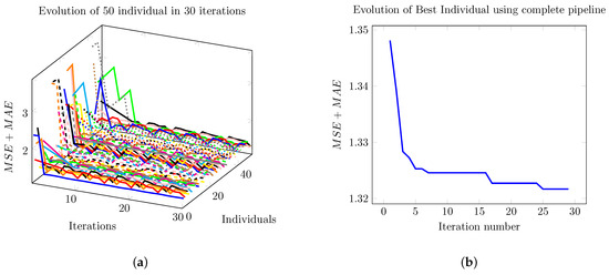
Figure 10.
Evolution of the PSO algorithm. Using this optimization algorithm, we selected the best set of parameters for the model. We set the number of individuals, that is, independent realizations, to 50. (a) Evolution of the depth error (MSE + MAE) of each of the 50 model parameters candidates and the error evolution over successive iterations. (b) For clarity, the evolution of the best individual from the previous 50 shown in (a) is shown here.
In Figure 10a, we show the evolution of each candidate in the PSO algorithm. We use 50 individuals, i.e., we have 50 curves in 30 iterations. Each individual is a possible parameter set that minimizes the error function, Equation (31). The evolution of each individual follows the dynamics given by Equations (32) and (33). In each iteration, we compute the performance of each individual or fitness as plotted in Figure 10a. In Figure 10b, we show the fitness of the best individual for all iterations.
The PSO algorithm was selected because most of the parameters are real numbers. We discarded other optimization methods that use discrete domains, such as the genetic algorithm. In a previous work [3], we implemented and tested the Elephant Herd Optimization (EHO) algorithm as an alternative to the PSO algorithm. The results showed that the EHO was less effective than the PSO algorithm at optimizing our objective function.
4.1. Model Training Difficulties
Several difficulties were encountered during the training process, mainly due to the initialization of the model’s parameters. Some of them are detailed as follows:
- 1.
- In the training stage, we initialized the PSO with 50 instances, with each instance being a set of random values for the parameters. Some combinations of these parameters generated invalid models or, in other words, NaN (Not a number) values. CUDA and MATLAB can handle NaN values, but when MSE and MAE were computed, invalid models received a performance value of MAX_PERFORMANCE.
- 2.
- When we initialized PSO instances, for each component of the instance (or parameter), we considered a random value from the MIN_VALUE - MAX_VALUE range. This fact restricted the initial values to be positive and within reasonable ranges.
- 3.
- We limited the velocity of the PSO instances using Equation (32), using a value between −2 and 2.
- 4.
- Depth data in the data set are provided in binary format, representing an image containing a long integer. Each image was converted from long integer format to floating-point values and saved as a text file. Our code read this text file and completed the depth data. The output of the model was a floating-point image.
4.2. Experiments
We trained the model using the KITTI and the NYU_V2 data sets under the following different scenarios:
- 1.
- Using the KITTI data set considering the positive definite metric.
- 2.
- Using the KITTI data set considering the anisotropic metric.
- 3.
- Using the KITTI data set, considering the biased infinity Laplacian and the anisotropic metric.
- 4.
- Using the KITTI data set, considering the double biased infinity Laplacian and the anisotropic metric.
- 5.
- Using NYU_V2 downsampled 4× considering the positive definite metric.
- 6.
- Using NYU_V2 downsampled 4× considering the anisotropic metric.
- 7.
- Using NYU_V2 downsampled 8× considering the positive definite metric.
- 8.
- Using NYU_V2 downsampled 8× considering the anisotropic metric.
- 9.
- Using NYU_V2 downsampled 16× considering the positive definite metric.
- 10.
- Using NYU_V2 downsampled 16× considering the anisotropic metric.
- 11.
- Using the KITTI data set, we varied the number of images in the training set considering the anisotropic metric.
Considering each trained model from (1) to (12), we performed the experiments on the KITTI and NYU_V2 data sets, as summarized in Table 5.
Table 5.
Experiments performed with our model in order to obtain MSE + MAE.
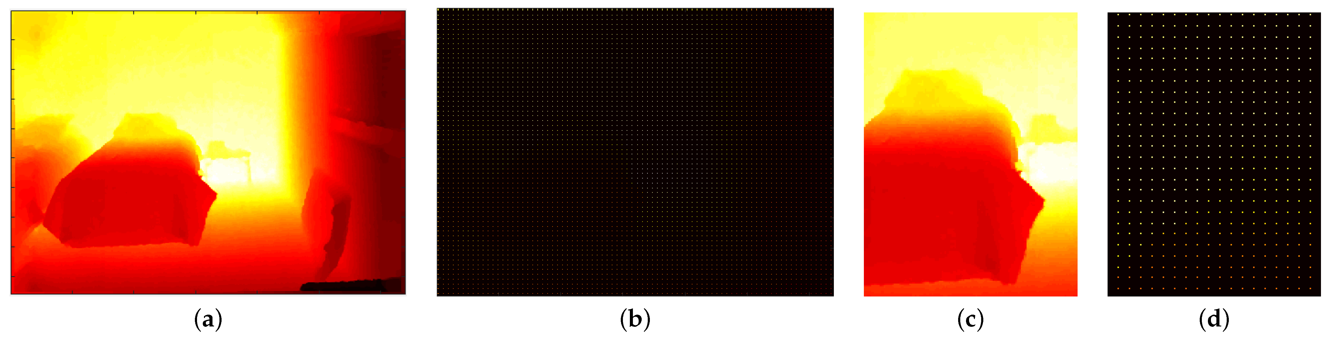
Figure 11 shows an example of the subsampled depth map. In Figure 11a, we show the ground truth acquired with a Kinect sensor. In Figure 11b, we show the subsampled depth map; we took one sample every other square pixel. Figure 11c shows a cropped area of Figure 11a and a subsampled version of Figure 11c.

Figure 11.
Example of the subsampled image. We sampled the original depth map in (a) every other (or ) square pixel in (b). In (c), we zoom in on a region (on the bed) of the depth map in (a). In (d), we show a zoom of the downsampled depth map in (c).
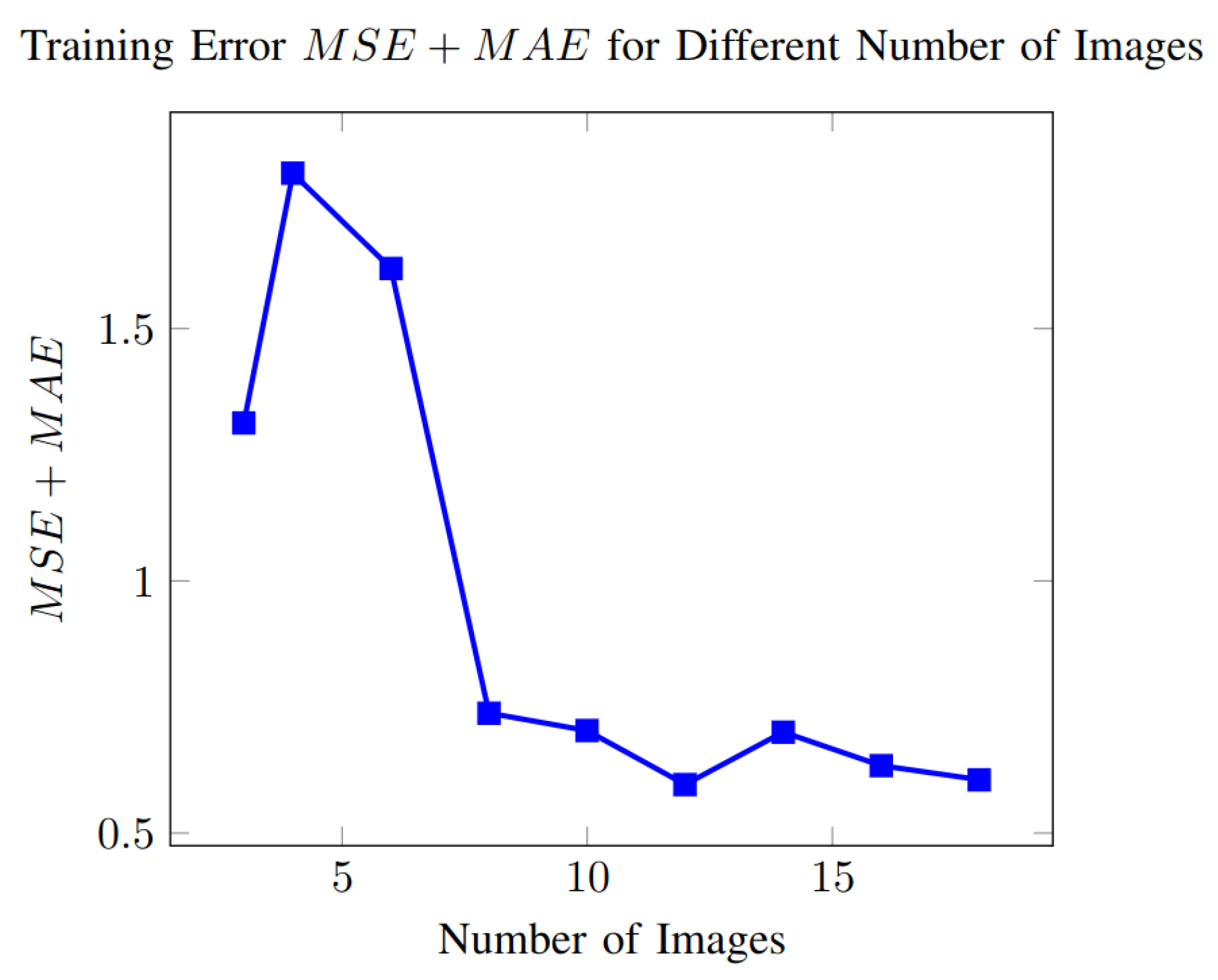
Experiment number 11 considers a varying number of images in the training set. We trained the model using sets containing 3 to 18 images. In Figure 12, we show the error for different numbers of images.
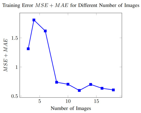
Figure 12.
Error in the training set as a function of the number of images in the training set.
Figure 12 shows the training error as a function of the number of images. The figure shows the variability in the error. The fluctuation in the curve is due to the PSO algorithm’s random nature and the images’ natural variation. We mention that as we increased the number of images in the training set, the best-selected individual tended to require a large number of iterations for the model to converge, from 92 iterations with three images to 170 iterations with eight images, slowing down the interpolation of the depth map. Furthermore, the other candidate solutions also required a large number of iterations, contributing to the slower convergence of the PSO algorithm.
5. Results
This section summarizes the quantitative and qualitative results obtained for the KITTI and the NYU_V2 data sets.
The KITTI data set contains depth data acquired by the LiDAR sensor. Holes in depth data can be caused by the occlusion between objects in the scene, sensor misinterpretation, transparent objects, reflections, and other effects. In Figure 13, we show examples of this lack of information, showing the reference color image and the depth ground truth.
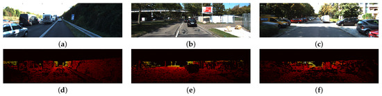
Figure 13.
Examples of lack of information in depth maps. Figures (a–c) show reference color images. Figures (d–f) show depth map ground truth.
Figure 13 shows color reference images and the corresponding depth ground truth. In (a), we observe (to the left) a black van, which is highly reflective. In (d), the corresponding depth data present holes on the van surface. LiDAR failed to measure depth information on that reflective surface. Additionally, occlusion between objects created a lack of depth information below the protective railing on the right of the image. In Figure 13b,e, we observe a reflective black car and, to the right, two rocks on a white horizontal flat surface. The depth map in (Figure 13e) presents holes in the corresponding location of the black van and on the white reflective surface. In Figure 13c,f, we observe that the depth map on the yellow car (left) presents holes in its glasses due to transparent objects. Also, we observe a similar lack of information on the gray car to the right.
5.1. Results Obtained in KITTI Depth Completion Suite
We processed the complete KITTI data set and obtained the and . In Table 6, we show the and for our proposal, as well as for other models, such as Deep Fusion, Morphological Operators neural networks [23], and Convolutional Spatial Propagation Networks [24].
Table 6.
Depth Completion Error in KITTI data set.
Table 6 shows the quantitative results of our proposal compared to other state-of-the-art models. Our three proposals outperform our previous work, already presented in [1], performing better than the model considering the Texture+Structure decomposition. Comparing our results with other models, we observe that our proposals outperform Deep Fuse Networks [13] and perform similarly to Convolutional Spatial Propagation Networks [24] and Morpho Networks [23]. We emphasize that our proposals are straightforward and fast to implement. Completing involves a simple weighted average and an iterative procedure.
Table 6 shows that the proposed anisotropic metric model is our best proposal considering MSE+MAE. It is noteworthy that the model presenting the best performance is the simplest one, i.e., infinity Laplacian and the anisotropic metric.
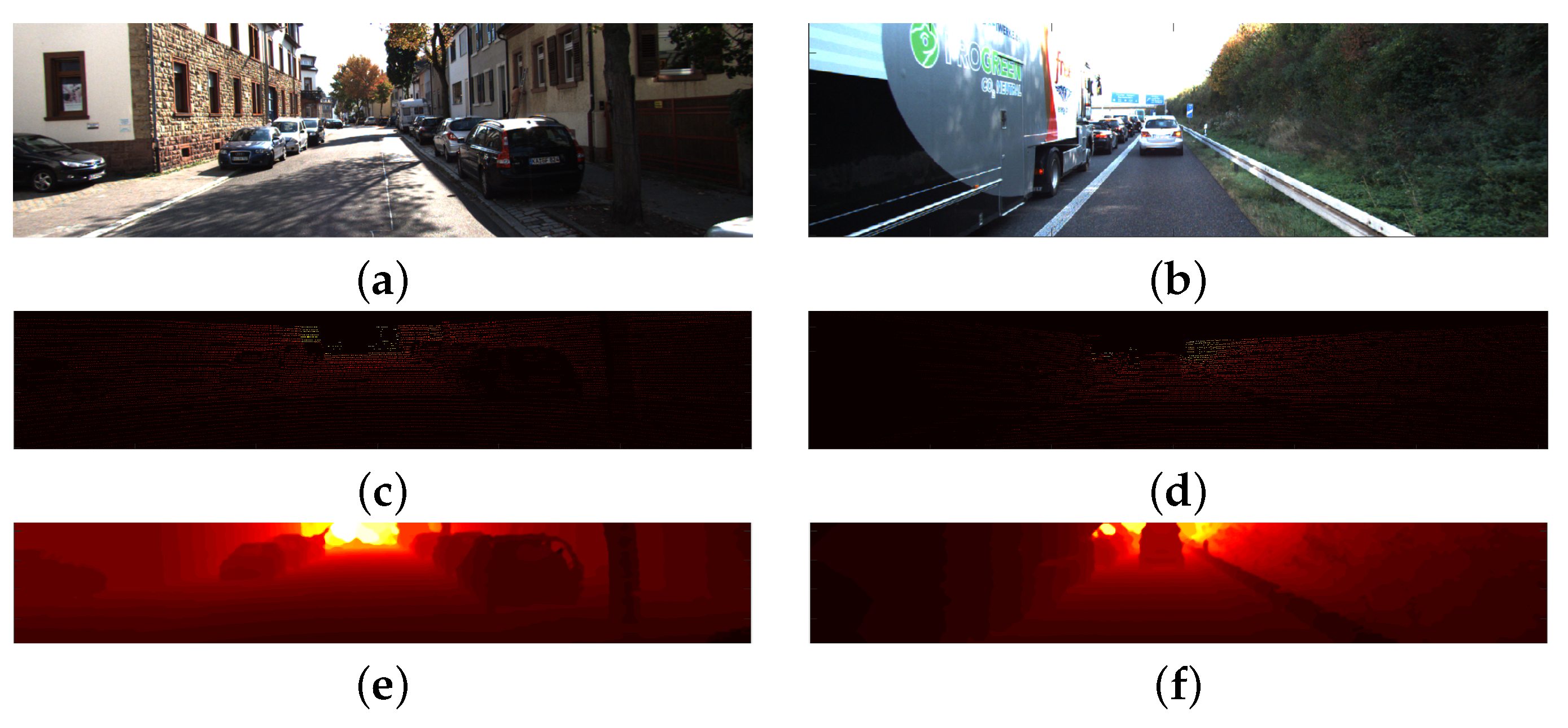
In Figure 14, we show qualitative results obtained by our models in the KITTI data set. Figure 14e,f show the minimum MSE obtained by our model in the KITTI data set, with an error of 53.78 cm and 52.09 cm, respectively.
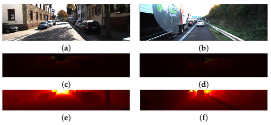
Figure 14.
Examples of qualitative and quantitative results obtained by our best model in the KITTI data set. We show color reference images in (a,b). In (c,d), we show the sparse depth map used as input to our model. In (e,f), we show the completed depth map and the obtained in each image.
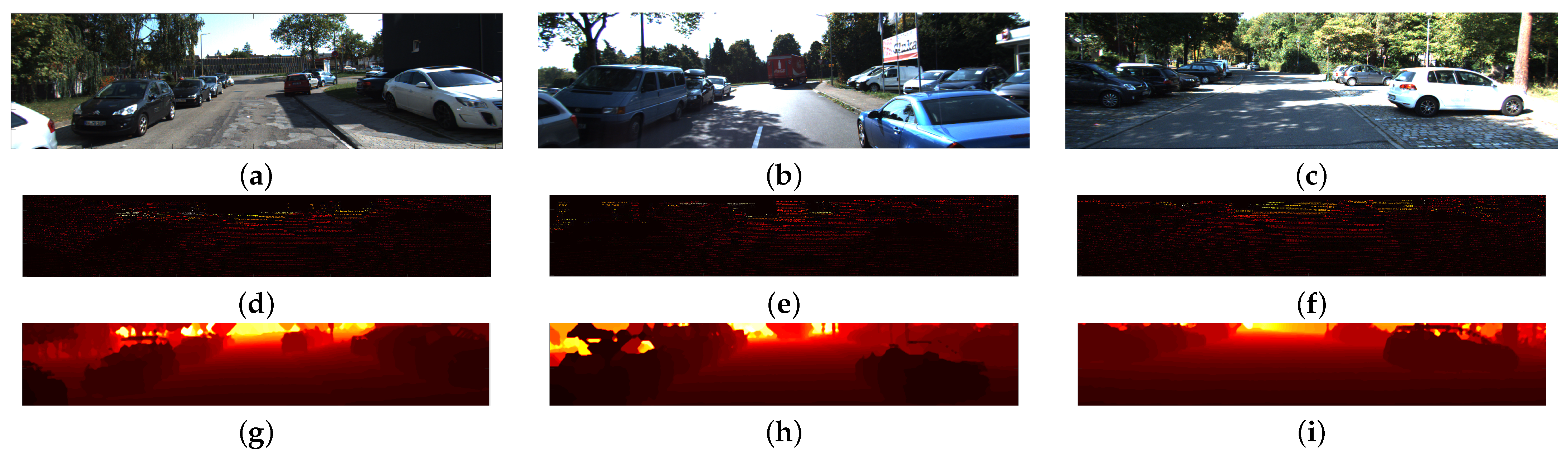
In Figure 15, we show qualitative results where our model fails to complete the task. In Figure 15g–i, we observe that our model cannot recover the car geometry due to transparent objects or excessive reflections. In these three images, we obtained the most significant errors. In (g) we obtained , in Figure 15h we obtained , and in Figure 15i we obtained .

Figure 15.
Examples of qualitative and quantitative errors obtained by our model in the KITTI data set. We show our worst results in the KITTI data set. In (a–c), we show color reference images. We present the sparse depth map used as input to our model in (d–f). In (g–i), we show the completed depth map.
5.2. Experiments Varying the Number of Images in the Training Set
Experiment 11 involved varying the number of images in the training set. We trained the model and then we evaluated the model using the complete KITTI data set.
In Table 7, we show the experiment’s results.
Table 7.
Depth Completion Error obtained varying the number of images in the training set.
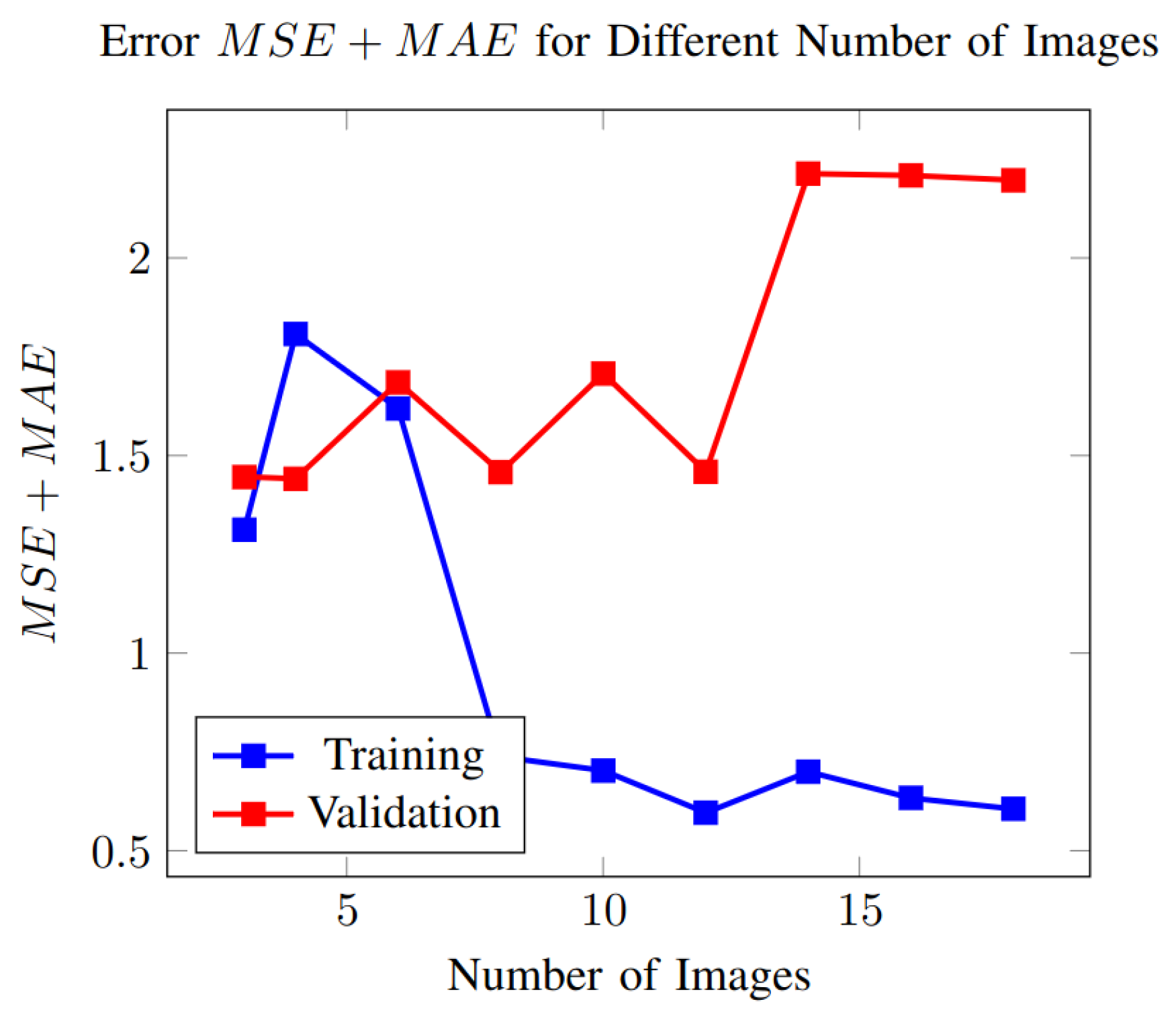
In Figure 16, we simultaneously plot the obtained results in Figure 12 and Table 7. We show the results in the training set and in the validation set.
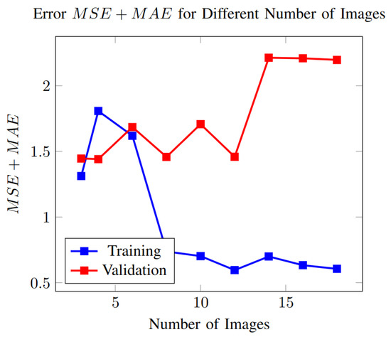
Figure 16.
Error in the training and validation set as a function of the number of images in the training set.
In Figure 16, we observe that as the number of training images increases, the training error decreases and finally saturates (curve in blue). However, the error in the validation set tends to increase as the number of images grows (curve in red). This behavior shows the model is overfitting to the training set. To obtain better results with a large set of training images, the PSO algorithm may overfit the model, i.e., it can reach with ten images.
Considering three or four images in the training set, we had higher training errors; however, we obtained the minimum error in the validation set.
This study highlights the trade-off between good performance in the training set and good performance in the validation set. Therefore, our decision to take three images in the training set is supported by the fact that it leads to the best performance in the validation set and suggests more generalization capabilities.
5.3. Results Obtained in NYU _V2
Table 8 shows our results for different subsampling factors in the upsampling task. We compare the results obtained by our proposal with different models available in the literature regarding the completion error ().
Table 8.
Depth Completion Error obtained by different models in NYU_V2.

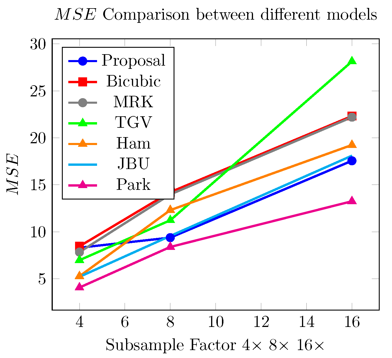
Figure 17.
Comparison of obtained between models: Our proposal, Bicubic, TGV [10], Ham [28], JBU, and Park [2].
In Figure 17, we observe that our proposal (in blue) outperforms the model Total Generalized Variation [10], Filtering using static and dynamic guidance [28], and Bicubic interpolation for upsampling factors of 8× and 16×. The JBU and Ham models [28] perform better than ours.
In Figure 18, we show quantitative and qualitative results obtained by the proposal on the images already presented above in Figure 9. Depth maps were downsampled by a factor of eight.
Figure 18 shows color frames and their corresponding interpolated depth maps. Figure 18g shows the completed depth map of the downsampled depth map. Similar results are presented in Figure 18h,i.
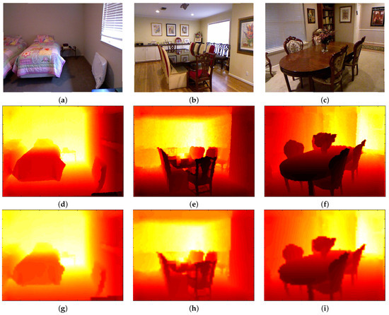
Figure 18.
Examples of completed depth maps in the NYU_V2 data set. Figures (a–c) show examples of three color reference images, and (d–f) show their corresponding ground truth, respectively. In (g), we obtained an , in (h) we obtained , and in (i) we obtained . In these figures, we show the completed depth maps with an upsampling factor of .
5.4. Ablation Test
We performed an ablation test on our proposed model. In this ablation test, we used the NYU_V2 data set with a factor . In each evaluation, we disabled one of the stages of the model while keeping the other stages active. In each test, we turned off the convolution stage (CS1) and the convolutional stage (CS2). We show the results of the ablation test in Table 9.
Table 9.
Results of the ablation test.
In Table 9, we show the results of the ablation test. By turning off the convolutional stage CS1, we observe that the MSE increases by 0.0146 cm; by changing the anisotropic metric for the previous metric, the MSE increases by 0.0004 cm. Turning off the convolutional stage CS2, the MSE error increases by 0.3393 cm. These increments show that given the data set NYU_V2 and the estimated parameters, the most critical stage of the proposal is the final stage, which eliminates outliers and noise.
5.5. Discussion
In summary, we present the results obtained by our proposal in the KITTI data set and in the NYU_V2 data set in Table 10 and Table 11, respectively.
Table 10.
Best results obtained in KITTI data set.
Table 11.
Best results obtained in NYU_V2 data.
In Table 10, in the second row, we show the results obtained by our proposal in the KITTI data set. We obtained an in the KITTI data set, outperforming our previous published version of the model in [1] () and other similar contemporaneous models [13]. In Table 11, in the NYU_V2 data set, we obtained s of 8.31, 9.35, and 17.56 with an upsampling factor of , 8×, and 16×, respectively. Our results outperform many contemporaneous models, such as [28] and [10].
Last but not least, we would like to mention the main limitations of our model and our evaluation:
- 1.
- The model struggled to accurately fill in objects with weak edges in the reference image. In the case of objects with weak edges, the model failed to accurately propagate the depth information correctly, causing data from different objects to merge. A possible solution to tackle this problem could be to use a semantic segmentation of the reference color image and use superpixel boundaries in order to stop diffusion.
- 2.
- The model faced challenges when dealing with transparent and reflective objects. We will tackle this problem in our future work.
- 3.
- Performance was evaluated using only two data sets. We consider that having only two data sets is insufficient to generalize our conclusions. Therefore, we plan to extend the evaluation to more data sets. In any case, the preliminary results are promising, particularly in using this technique in real-world scenarios and applications such as 3D reconstruction of an urban scene. An example of the depth completion for an urban scene is shown in Figure 19.
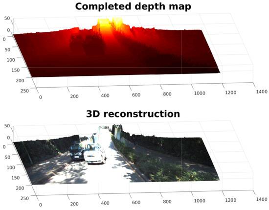 Figure 19. A 3D reconstruction of an urban scene from a depth map and a color frame. The first row shows the 3D interpolated depth of an urban scene. The second row shows the reconstruction of the 3D scene created using the color reference and the completed depth map.
6. Conclusions
This paper extends the work presented in [1], evaluating new variations of the original model to interpolate incomplete depth maps. The results have been qualitatively and quantitatively evaluated in two data sets, KITTI and NYU_V2.
The main conclusions of this work are as follows: (i) the use of an anisotropic metric improves model performance; (ii) the use of a Texture+Structure decomposition as a pre-filtering stage did not have a significant impact; and (iii) the ablation test showed that the model’s final stage is an essential component in the pipeline, with its suppression leading to an increase of approximately 4%. We also show that our model outperforms state-of-the-art alternatives with similar levels of complexity.
The model shows a performance superior to or at least similar to other state-of-the-art algorithms that are not based on deep neural networks. Nevertheless, its complexity and execution were significantly faster than those approaches, outperforming most of them by an order of magnitude. In the context of the current evaluation, our approach outperformed TGV [10] and JBU in the NYU_V2 data set, and is comparable to Morpho Networks [23] and Convolutional Spatial Networks [24].
We varied the number of images included in the training set. The results show that as the number of considered images grows, the PSO algorithm tends to overfit the model to obtain better results in the training set. This fact comes at the expense of compromising the model’s performance in the validation test. The model achieves acceptable performance when using only three images for training. For training sets using more than three images, the PSO algorithm selects the best parameters, which present a large number of iterations, increasing the complexity of the model, making the execution of the model run slowly and be more demanding on computational resources.
A hybrid approach is advantageous as it combines the generalization capabilities of classical models with the high precision provided by new features obtained through convolutional stages. Also, the flexible structure of the pipeline lets the model reach its maximum performance considering the used interpolation model.
Experimentally, we evaluated the model only in two data sets: KITTI and NYU_V2. In order to assess the generalization capabilities of the model, it is necessary to extend the evaluation to other contemporary data sets, such as Middlebury or Virtual KITTI. Furthermore, the parameter estimator (PSO) has additional parameters that require optimization. We think it is possible to obtain better performance by optimizing the parameters of the PSO algorithm. We propose investigating nested optimization to jointly estimate both the parameters of the model and those of the PSO algorithm.
Future work will consider the implementation of a better approximation of the geodesic distance, evaluating the model in other data sets (synthetic and real data sets), and matching patches instead of matching individual pixels. When we determine the that maximizes the positive eikonal operator and the that minimizes the negative eikonal operator, we compare pixels; more robust matching could be performed using patches instead of matching pixels. This fact will increase the confidence of the matching.
We will also improve the model’s result in areas of the color image with weak boundaries and in the presence of transparency and intense reflections.
Author Contributions
The development of this work, F.C. and V.L.; contribution to conceptualization, V.L. and F.C.; methodology, V.L. and F.C.; software, V.L.; validation, V.L.; analysis, F.C.; bibliography and references, V.L. and F.C.; writing—original draft preparation, V.L. and F.C.; review and editing, F.C. All authors have read and agreed to the published version of the manuscript.
Funding
This research received no external funding.
Institutional Review Board Statement
Not applicable.
Informed Consent Statement
Not applicable.
Data Availability Statement
The data presented in this study are available in The KITTI Vision Bench-mark Suite at https://www.cvlibs.net/datasets/kitti/eval_depth.php?benchmark=depth_completion and NUYDepthDatasetV2 at https://cs.nyu.edu/~fergus/datasets/nyu_depth_v2.html, accessed on 23 April 2024.
Conflicts of Interest
The authors declare no conflicts of interest.
References
- Lazcano, V.; Calderero, F. Hybrid Model Convolutional Stage-Positive Definite Metric Operator-Infinity Laplacian Applied to Depth Completion. In Proceedings of the IEEE 2022 Tenth International Symposium on Computing and Networking Workshops (CANDARW), Himeji, Japan, 21–24 November 2022; pp. 174–179. [Google Scholar] [CrossRef]
- Park, J.; Kim, H.; Yu-Wing, T.; Brown, M.; Kweon, I. High quality depth map upsampling for 3D-TOF cameras. In Proceedings of the 2011 International Conference on Computer Vision, IEEE, Barcelona, Spain, 6–13 November 2011; pp. 1623–1630. [Google Scholar] [CrossRef]
- Lazcano, V.; Calderero, F.; Ballester, C. Comparing Different Metrics on an Anisotropic Depth Completion Model. Int. J. Hydrid Intell. Syst. 2021, 17, 87–99. [Google Scholar] [CrossRef]
- Lu, K.; Barnes, N.; Anwar, S.; Zheng, L. From Depth What Can You See? Depth Completion via Auxiliary Image Reconstruction. In Proceedings of the IEEE/CVF Conference on Computer Vision and Pattern Recognition (CVPR), IEEE, Seattle, WA, USA, 13–19 June 2020. [Google Scholar]
- Geiger, A.; Lenz, P.; Stiller, C.; Urtasun, R. Vision meets Robotics: The KITTI Dataset. Int. J. Robot. Res. (Ijrr) 2013, 32, 1231–1237. [Google Scholar] [CrossRef]
- Li, Y.; Huang, J.B.; Ahuja, N.; Yang, M.H. Joint Image Filtering with Depth Convolutional Networks. Trans. Pattern Anal. Mach. Intell. 2019, 41, 1909–1923. [Google Scholar] [CrossRef] [PubMed]
- Lai, W.S.; Huang, J.B.; Ahuja, N.; Yang, M.H. Fast and accurate Image Super-Resolution with Deep Laplacian Pyramid Network. Trans. Pattern Anal. Mach. Intell. 2019, 41, 2599–2613. [Google Scholar] [CrossRef] [PubMed]
- Imran, S.; Long, Y.; Liu, X.; Morris, D. Depth Coefficients for Depth Completion. In Proceedings of the IEEE Conference on Computer Vision and Pattern Recognition, Long Beach, CA, USA, 15–20 June 2019; pp. 12438–12447. [Google Scholar]
- Zhang, Y.; Funkhouser, T. Deep depth completion of a single rgb-d image. In Proceedings of the IEEE Internatinal Conference on Computer Vision and Pattern Recognition, Salt Lake City, UT, USA, 18–22 June 2018. [Google Scholar]
- Ferstl, D.; Reinbacher, C.; Ranftl, R.; Ruether, M.; Bischof, H. Image Guided Depth Upsampling Using Anisotropic Total Generalized Variation. In Proceedings of the 2013 IEEE International Conference on Computer Vision, Sydney, NSW, Australia, 1–8 December 2013; pp. 993–1000. [Google Scholar] [CrossRef]
- Xu, Y.; Zhu, X.; Shi, J.; Zhang, G. Depth completion from sparse lidar data with depth-normal constraints. In Proceedings of the International Conference on Computer Vision, Seoul, Republic of Korea, 27 October–2 November 2019. [Google Scholar]
- Park, J.; Joo, K.; Hu, Z.; Liu, C.; Kweon, I.S. Non-local spatial propagation network for depth completion. In Proceedings of the European Conference on Computer Vision, Glasgow, UK, 23–28 August 2020. [Google Scholar]
- Shivakumar, S.; Nguyen, T.; Miller, I.; Chen, S.; Kumar, V.; Taylor, C. DFuseNet: Deep Fusion of RGB and Sparse Depth Information for Image Guided Dense Depth Completion. In Proceedings of the 2019 IEEE Intelligent Transportation Systems Conference (ITSC), Auckland, New Zealand, 27–30 October 2019; pp. 13–20. [Google Scholar] [CrossRef]
- Hu, M.; Wang, S.; Li, B.; Ning, S.; Fan, L. Penet: Towards precise and efficient image guided depth completion. In Proceedings of the International Conference on Robotics and Automation, Xi’an, China, 30 May–5 June 2021. [Google Scholar]
- Lin, Y.; Cheng, T.; Zhong, Q.; Zhou, W.; Yang, H. Dynamic Spatial Propagation Network for Depth Completion. In Proceedings of the AAAI 2022 Conference on Artificial Intelligence, Virtual, 22 February–1 March 2022. [Google Scholar]
- Tang, J.; Tian, F.; Feng, W.; Li, J.; Tan, P. Learning guided convolutional network for depth completion. IEEE Trans. Image Process. 2021, 30, 1116–1129. [Google Scholar] [CrossRef] [PubMed]
- Bai, L.; Zhao, Y.; Elhousni, M.; Huang, X. DepthNet: Real-Time LiDAR Point Cloud Depth Completion for Autonomous Vehicles. IEEE Access 2020, 8, 227825–227833. [Google Scholar] [CrossRef]
- Caselles, V.; Igual, L.; Sander, O. An axiomatic approach to scalar data interpolation on surfaces. Numer. Math. 2006, 102, 383–411. [Google Scholar] [CrossRef]
- Lazcano, V.; Calderero, F.; Ballester, C. Depth Image Completion Using Anisotropic Operators. In Proceedings of the 12th International Conference on Soft Computing and Pattern Recognition (SoCPaR 2020). Advances in Intelligent Systems and Computing; Springer: Cham, Switzerland, 2020. [Google Scholar]
- Krauss, B.; Schroeder, G.; Gustke, M.; Hussein, A. Deterministic Guided LiDAR Depth Map Completion. In Proceedings of the IEEE Intelligent Vehicles Symposium (IV), Nagoya, Japan, 11–17 July 2021; pp. 824–831. [Google Scholar] [CrossRef]
- Saidi, T.; Kohuas, A.; Amira, A. Implementation of a real-time stereo vision algorithm on a cost-effective heterogeneous multicore platform. Concurr. Comput. Pract. Exp. 2023, 35, 1–22. [Google Scholar] [CrossRef]
- Eldesokey, A.; Felsberg, M.; Holmquist, K.; Persson, M. Uncertainty-Aware CNNs for Depth Completion: Uncertainty from Beginning to End. In Proceedings of the IEEE/CVF Conference on Computer Vision and Pattern Recognition (CVPR), Seattle, WA, USA, 13–19 June 2020. [Google Scholar]
- Dimitrievski, M.D.; Veelaert, P.; Philips, W. Learning Morphological Operators for Depth Completion. In Proceedings of the Advanced Concepts for Intelligent Vision Systems Conference, Poitiers, France, 24–27 September 2018; IEEE: Piscataway, NJ, USA. [Google Scholar]
- Cheng, X.; Wang, P.; Yang, R. Learning Depth with Convolutional Spatial Propagation Network. IEEE Trans. Pattern Anal. Mach. Intell. 2020, 42, 2361–2379. [Google Scholar] [CrossRef] [PubMed]
- Silberman, N.; Hoiem, D.; Kohli, P.; Fergus, R. Indoor Segmentation and Support Inference from RGBD Images. In Proceedings of the ECCV, Firenze, Italy, 7–13 October 2012. [Google Scholar]
- Lazcano, V.; Ramírez, I.; Calderero, F. Anisotropic Operator Based on Adaptable Metric-Convolution Stage-Depth Filtering Applied to Depth Completion. In Pattern Recognition; Lu, H., Blumenstein, M., Cho, S.B., Liu, C.L., Yagi, Y., Kamiya, T., Eds.; Springer: Cham, Switzerland, 2023; pp. 1–14. [Google Scholar]
- Lazcano, V.; Calderero, F. A Discussion on Variants of an Anisotropic Model Applied to Depth Completion. In Advanced Research in Technologies, Information, Innovation and Sustainability; Guarda, T., Portela, F., Diaz-Nafria, J.M., Eds.; Springer: Cham, Switzerland, 2024; pp. 3–16. [Google Scholar]
- Ham, B.; Cho, M.; Ponce, J. Robust image filtering using joint static and dynamic guidance. In Proceedings of the IEEE Conference on Computer Vision and Pattern Recognition, Boston, MA, USA, 7–12 June 2015. [Google Scholar]
- Li, Y.; Huang, J.; Ahuja, N.; Yang, M. Deep Joint Image Filtering. In Computer Vision—ECCV 2016; Leibe, B., Matas, J., Sebe, N., Welling, M., Eds.; Springer: Cham, Switzerland, 2016; pp. 154–169. [Google Scholar]


Disclaimer/Publisher’s Note: The statements, opinions and data contained in all publications are solely those of the individual author(s) and contributor(s) and not of MDPI and/or the editor(s). MDPI and/or the editor(s) disclaim responsibility for any injury to people or property resulting from any ideas, methods, instructions or products referred to in the content. |
© 2024 by the authors. Licensee MDPI, Basel, Switzerland. This article is an open access article distributed under the terms and conditions of the Creative Commons Attribution (CC BY) license (https://creativecommons.org/licenses/by/4.0/).