Abstract
Although deep neural networks have been successfully applied in many fields, research studies show that neural network models are easily disrupted by small malicious inputs, greatly reducing their performance. Such disruptions are known as adversarial attacks. To reduce the impact of adversarial attacks on models, researchers have proposed adversarial training methods. However, compared with standard training, adversarial training results in additional computational overhead and training time. To improve the training effect without significantly increasing the training time, an improved Fast-M adversarial training algorithm based on the fast adversarial training algorithm is proposed in this paper. Extensive comparative experiments are conducted with the MNIST, CIFAR10, and CIFAR100 datasets. The results show that the Fast-M algorithm achieves the same training effect as the commonly used projected gradient descent (PGD) adversarial training method, with a training time that is only one-third of that of PGD and a performance comparable to that of fast adversarial training, demonstrating the proposed algorithm’s effectiveness.
1. Introduction
The rise of deep learning has led to rapid developments in the field of artificial intelligence, attracting an increasing number of researchers to the field. At the same time, the number of fields in which deep learning is being applied is constantly increasing; such fields include image classification, object detection, autonomous driving, and natural language processing. However, while deep learning technology is seemingly successful, like most traditional internet technologies, it also has its own shortcomings and security issues [1].
Szegedy et al. [2] made a discovery in image classification using deep neural net-works; by adding specific, imperceptible perturbations to an original image that can be successfully classified by a neural network model and then classifying the perturbed im-age with the same model, the result obtained is completely different from that before. This indicates that seemingly small perturbations easily interfere with neural network models, leading to a significant drop in classification accuracy. Goodfellow et al. [3] called these data perturbations that produce classification errors “adversarial examples”, officially introducing the concept of adversarial attacks. Since then, many researchers have started working in this field.
Determining the extent to which deep neural network models resist adversarial at-tacks is called the robustness problem of deep neural networks, which is still a very active research area, especially in some application fields that prioritize security and safety, such as facial recognition, autonomous driving, and object detection [4]. The goal of improving neural network robustness is to train a robust neural network model or to add a detection mechanism when processing data inputs, so that the neural network model is accurate not only for the original data but also for data with adversarial perturbations. To this end, researchers have proposed many methods, such as defensive distillation [5], adversarial detection [6,7], sample randomization [8], and adversarial training, to improve the robustness of deep neural network models. Currently, adversarial training is considered the most effective among these methods of defense and is the main focus of this article.
To improve the training effect without significantly increasing the training time, this paper proposed an improved Fast-M adversarial training algorithm based on the fast adversarial training paradigm. The main contributions are summarized as follows:
- This paper analyzes the differences between PGD adversarial training and free and fast adversarial training in training overhead and discusses the influence of the step size and the number of iterations on the training performance.
- This paper proposes an improved Fast-M adversarial training algorithm based on the fast adversarial training method to reduce the computational overload while maintaining the training performance.
- Extensive experiments are conducted with the MNIST, CIFAR10, and CIFAR100 datasets. Results show that the Fast-M algorithm achieves the same training effect as the commonly used adversarial training method, with a training time that is only one-third that of PGD adversarial training.
2. Related Work
The earliest adversarial training method [3] was proposed by using the fast gradient sign method (FGSM) to add adversarial perturbations during model training to enhance model robustness. However, as increasingly powerful adversarial attack algorithms appeared, this training method was quickly defeated by stronger adversarial attacks. Therefore, this training method is now considered an ineffective adversarial training method. Madry et al. [9] proposed the projected gradient descent (PGD) method, which is currently the most effective adversarial training method, and applied it to adversarial training. However, PGD often increases the training time by an order of magnitude compared to standard training, resulting in significant computational overhead and making it difficult to deploy for adversarial training on some larger networks. To address this difficulty, much work has been studied on how to reduce the runtime of adversarial training while still achieving high model robustness.
Shafahi et al. [10] proposed the free adversarial training method, which trains a robust CIFAR10 model. It took 785 min to achieve a maximum accuracy of approximately 46% under a PGD adversarial attack with and 20 iterations, while PGD-7 adversarial training required 5418 min to obtain the same accuracy, which shows that the same training result as that of PGD training can be obtained while reducing the training time. Wong et al. [4] introduced cyclic learning rates [11] and mixed-precision training [12] into adversarial training and applied them to PGD and free adversarial training methods, achieving a significant acceleration of both training methods and greatly reducing the time required for adversarial training. Ye et al. [13] proposed the Amata adversarial training method, which for the first time introduced the idea of a simulated annealing algorithm into adversarial training. Based on PGD adversarial training, Amata changes the number of iterations and training step size of PGD adversarial training in stages. Amata successfully trained a model with the same training effect as PGD-10 adversarial training in approximately half the time. However, compared with fast adversarial training, it still added more training time.
Gaurang et al. [14] proposed the GAMA (guided adversarial margin attack) adversarial attack methodology. GAMA builds upon the fundamental principles established by prior adversarial attacks like the fast gradient sign method (FGSM) and projected gradient descent (PGD), elevating them with a refined relaxation technique that guides the optimization process towards the creation of more potent adversarial perturbations. Additionally, Gaurang et al. proposed Guided Adversarial Training (GAT), a pioneering adversarial training approach that harnesses the power of GAMA, enabling the creation of robust models that exhibit remarkable performance even when faced with contemporary defenses. Notably, this contribution tackles the challenge of gradient masking commonly encountered in single-step training methods, offering a practical solution that enhances the dependability of deep networks in the presence of adversarial attacks.
From the various adversarial training methods mentioned above, it is not difficult to see that the goal of adversarial training is to achieve better training results with less training time, and the above methods do not balance training time and training effectiveness. If the training effect of PGD-7 is taken as the standard, although the training time of fast adversarial training is much shorter than that of PGD-7, its training effect is poorer. While training methods such as Amata can achieve a training effect comparable to that of PGD-7, the training time is still several times that of fast adversarial training, requiring significant computational costs. Therefore, to enhance the adversarial training effect while minimizing training time, this paper proposes the Fast-M adversarial training algorithm. The effectiveness of the proposed algorithm is verified in experimental environments.
3. Preliminary
3.1. Adversarial Attack
Adversarial attack refers to adding a certain perturbation to an image with the true label under the condition of a fixed classifier with parameters and a classification loss function to generate a new image sample that can cause classification errors in the classifier . The original image is called the original sample, while the new image , generated after adding , is called the adversarial sample. This problem can be expressed in the following form:
where represents a specific norm; here, , , and can be chosen as the space. The most commonly used norm is the norm, and limits the range of the perturbation .
After Szegedy et al. [2] discovered that neural network models are highly vulnerable to adversarial attacks, various adversarial attack algorithms emerged. Among them were many classical attack algorithms, including the fast gradient descent method (FGSM), basic iterative method (BIM) [15], DeepFool [16], C&W [17], projected gradient descent (PGD), one-pixel attack (OPA) [18], alternative black box attack (SBA) [19], zeroth order optimization (ZOO) [20], etc. Some of these typical adversarial attack algorithms are introduced below.
3.2. Fast Gradient Sign Method
The FGSM [3] is the earliest and most classic white-box gradient-based attack algorithm. It is a nontargeted attack algorithm. Its working principle is to give the model structure , weight parameters , and loss function and then compute the gradient with respect to the input . The sign vector of the gradient is multiplied by a very small positive number, which is the attack perturbation radius or attack step size , to produce a small perturbation. Then, the perturbation is added to the original image to generate an adversarial example:
The FGSM algorithm is a very simple but effective attack method. The term in Formula (2) represents the first-order derivative with respect to the input x. It shows that only one backward propagation of the gradient is needed to achieve a successful attack. The reason this method is effective is that during the training of a neural network model, the model weights are updated in the direction of the gradient, reducing the loss value. Empirically, the smaller the model’s loss value is, the higher its classification accuracy. This method calculates an input that increases the model’s loss value along the direction of the gradient, and thus, in the case of a fixed network structure of the model, the loss value is increased, which leads to a significant decrease in the model’s accuracy for adversarial samples.
3.3. Projected Gradient Descent
The PGD method [9] is a nontargeted attack algorithm that uses the norm. Its principle is to first initialize a starting perturbation randomly near the original sample within the perturbation radius (a spherical noise region) and then compute the gradient of the perturbed sample. With a fixed attack step size , the perturbation is iteratively updated using Formula (2), and if the perturbation exceeds the attack perturbation radius , it is projected back to the corresponding position within . The perturbed sample is updated continuously until the iteration is finished or the best perturbation is obtained to generate an adversarial example. The PGD attack is currently the most powerful first-order norm attack. If a neural network model has good defense against PGD attacks, it also has good defense against other first-order attacks. Therefore, the PGD attack is often used to evaluate the robustness of models against adversarial defenses, and it is also one of the main evaluation criteria for the adversarial defense algorithms proposed in this paper.
4. Discussion of Typical Adversarial Training Algorithms
Madry et al. [9] proposed the “max-minimization model”, which was the first to transform adversarial training into a robust optimization problem. It can be represented by the following formula:
where is the original image, is the true label of , is the loss function, is the network model structure with weight parameters , is the adversarial perturbation to be added, and is the set of attack radii or perturbations. The goal of adversarial training is to find the point around the original data that maximizes the model’s loss and then update the model parameters to minimize the loss at that point. That is, by using powerful adversarial attack algorithms to generate optimal adversarial examples and then feeding them to the model for training, a robust model can be obtained. A key aspect of adversarial training is finding the point of internal loss maximization. Meanwhile, if the gradients within the attack radius are all zero and the loss values at each point are the same, then the model is perfectly stable within this attack radius.
4.1. PGD Adversarial Training
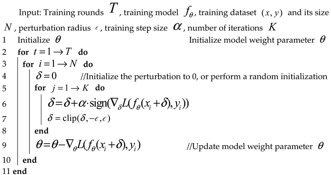
To achieve internal maximization in Formula (3), Madry et al. [9] proposed the PGD adversarial attack algorithm mentioned earlier. During training, a -step PGD attack is used to approximately maximize the internal loss and obtain the best adversarial sample. Then, the adversarial samples are used to update the model’s weight parameters. The specific implementation is shown in Algorithm 1. Compared to conventional standard training, PGD adversarial training usually takes times longer due to the additional gradient computations in each training round.
| Algorithm 1. K-Step PGD Adversarial Training | |||
 | |||
4.2. Free Adversarial Training
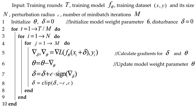
To reduce the time required for adversarial training, Shafahi et al. [10] proposed the free adversarial training method, which is shown in Algorithm 2. It uses the FGSM adversarial attack to compute iterations on a “mini-batch”. The perturbation is not reset between minibatches, and only one backward propagation is performed between iterations of a minibatch while computing the gradients of both the perturbation and the model. Therefore, rounds of free adversarial training are equivalent to rounds of standard training.
| Algorithm 2. Free Adversarial Training | |||
 | |||
4.3. Fast Adversarial Training
Wong et al. [4] believed that the key to the effectiveness of free adversarial training lies in the fact that the perturbation of each minibatch is not reset. The perturbation from the previous iteration is used as the initial starting point for the next iteration, which is equivalent to giving the perturbation of the FGSM attack a nonzero initialization. Therefore, they proposed fast adversarial training, which initializes the perturbation of each batch between and uses an FGSM attack for adversarial training. The implementation details are shown in Algorithm 3, where the clip in line 6 refers to a specific operation that limits the generated value range of the adversarial disturbance to , avoiding excessive noise in the generated image. Wong et al. [4] noted that fast adversarial training works best when the training step size . On the CIFAR10 dataset, a model trained for only 15 rounds can achieve 45% accuracy under 50 iterations of PGD attack with 10 random restarts. Moreover, one round of fast training takes the same time as two rounds of standard training, which is much less than the time required for PGD adversarial training.
| Algorithm 3. Fast Adversarial Training |
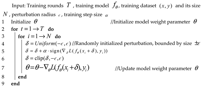 |
5. Fast-M Adversarial Training Algorithm
5.1. Design Rationale
Based on the previous discussion of the PGD adversarial training algorithm, free adversarial training algorithm, and fast adversarial training algorithm, it is easy to see that the main difference among them lies in the number of iterations for computing adversarial perturbations during training and the step size used for computing the perturbations. Specifically, PGD adversarial training uses a small step size with multiple iterations to compute adversarial perturbations, while fast adversarial training uses a large step size with a single iteration. These two methods use opposite approaches but achieve similar results, indicating that the key to adversarial training lies in the choice of the step size and number of iterations for each training round. Based on this analysis, an improvement to the fast adversarial training algorithm is proposed in this paper.
This paper considers adversarial training as a process in which the neural network model “grows” by updating its parameters after being repeatedly “defeated” by attack algorithms, thereby enhancing its defense capabilities against adversarial attacks. The model can only grow after being successfully “defeated”, which is a process of “finding and filling gaps”. The purpose of adversarial training is to proactively identify vulnerabilities in a neural network model that can be exploited by adversarial attack algorithms. Then, by updating the weight parameters, these vulnerabilities can be fixed, achieving “immunity” against adversarial attacks. Therefore, the key to adversarial training is to identify the model’s vulnerabilities, which is the same principle upon which the internal maximization in Formula (3) is based. To find the model’s vulnerabilities, an effective adversarial perturbation that can affect the model must be obtained.
5.2. Method
Inspired by the ideas of Ye et al. [13] regarding the impact of PGD adversarial training iterations on model robustness, this paper proposes replacing the simple increase in the internal adversarial perturbation calculation in fast adversarial training with staged increments. Fast adversarial training can be seen as giving one adversarial perturbation calculation to the neural network model in each round of training, where each round of training has an “even distribution”. However, adversarial training in the early stages of neural network model training has little effect on improving model robustness. Therefore, the proposed method removes the adversarial perturbation calculation iteration in the early stages of fast adversarial training to lower computational costs and increase the number of calculation iterations of the adversarial perturbation in the later stages of model training to obtain better adversarial samples and improve the robustness of the training model.
Based on the above points, this paper proposes a Fast-M adversarial training algorithm using the staircase iteration strategy, where denotes the predetermined number of stages. The core of this method is the strategy of calculating the number of iterations for adversarial perturbation calculation at different stages. The proposed method divides the total training rounds of the model’s adversarial training into stages, and the number of iterations for adversarial perturbation calculation at each stage is . The method adopts the approach of incrementally increasing the number of adversarial perturbation calculations for each stage. If the current training round is , the number of iterations for adversarial perturbation calculation at the current stage is , which is calculated with the following formula:
The difference between this strategy and the one in the Amata adversarial training method lies in the fact that the number of iterations in this strategy starts from 0. That is, the model’s adversarial training does not perform adversarial perturbation calculations in the first stage. Only the number of stages needs to be set, and the iteration number of each stage is calculated using the floor function. Therefore, the range of is .
The key to the Fast-M adversarial training algorithm is to use a fixed large attack step size and to increase the number of iterations in stages for adversarial training. The specific process is given in Algorithm 4.
| Algorithm 4. Fast-M Adversarial Training |
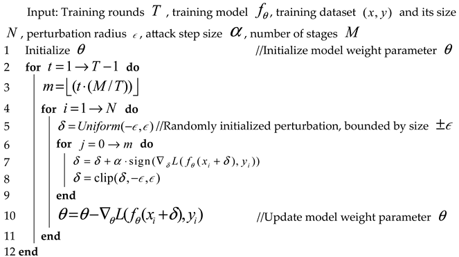 |
A round of fast adversarial training can be split into a standard training round and a round of FGSM adversarial perturbation calculation with random initialization. The main increase in training time compared to standard training is the time used for backward propagation in the additional round of FGSM adversarial perturbation calculation. For one of fast adversarial training, the additional backward propagation count is (assuming training on a complete dataset and ignoring the batch size). Therefore, if the Fast-M algorithm proposed in this paper is used for adversarial training, the total additional backward propagation count at is as follows:
Table 1 shows the total number of backward passes required for different training epochs and stage numbers , , and with Fast-M adversarial training. From the table, for , the number of required backward passes with our proposed algorithm is roughly the same as that with standard fast adversarial training. For , the number of backward passes is roughly the same as that with two-iteration fast adversarial training. Therefore, in theory, the training time of the Fast-3 algorithm is roughly the same as that of fast adversarial training, while the training time of the Fast-5 algorithm is close to the training time of two-iteration fast adversarial training.

Table 1.
Backward propagation times of fast adversarial training under different training epochs and different stage numbers .
.
6. Experiments
To verify the effectiveness of the Fast-M adversarial training algorithm, a series of comparative experiments are conducted with the MNIST, CIFAR10, and CIFAR100 datasets in this chapter. Multiple neural network models are trained using various adversarial training algorithms. Then, multiple adversarial attack algorithms are tested, and the results are compared and evaluated with respect to classification accuracy and training time against the results of the Fast-M adversarial training algorithm proposed in this paper. All experiments on the MNIST dataset were run on a laptop with 1 NVIDIA GTX 950 m, using LeNet as the backbone network. All experiments on the CIFAR10 dataset were run on a single server with an NVIDIA Tesla P100, using pretrained ResNet18 as the back-bone network. The experimental environment for both is Python 3.7. The deep learning framework is Pytorch 1.7.
6.1. Verification of Fast-M on MNIST
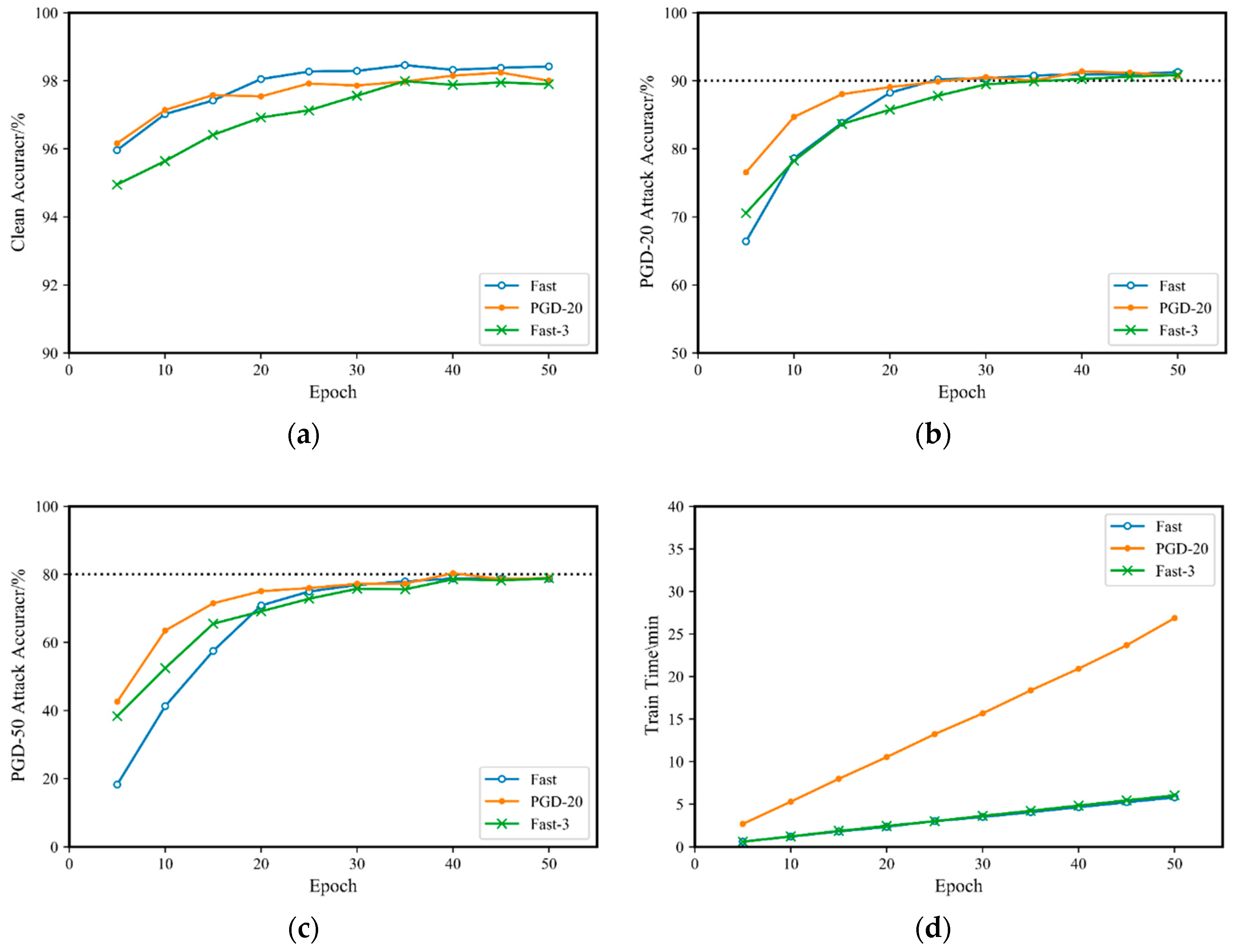
The performance of fast adversarial training on the MNIST dataset is comparable to that of PGD adversarial training but with significantly less time needed. This paper compares fast adversarial training, PGD-20 adversarial training, and the proposed Fast-M adversarial training on the MNIST dataset. Each of the three training methods is trained for 10 rounds of adversarial training, with the training epochs ranging from to . A model is trained every five rounds, resulting in a total of 10 models with different training epochs. The models are then evaluated, and the results are shown in Figure 1.
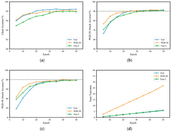
Figure 1.
Comparison of Fast-3 adversarial training and original fast adversarial training on the MNIST dataset.: (a) accuracy for the original clean sample; (b) accuracy for a PGD-20 attack; (c) accuracy for a PGD-50 attack; (d) training time.
From Figure 1b,c, the three adversarial training methods have similar defense capabilities against PGD adversarial attacks. With the increase in the number of training rounds, they all achieve 90% accuracy for PGD-20 and 80% accuracy for PGD-50 adversarial attacks. However, in the case of fewer training rounds, the training effect of Fast-M adversarial training is better than that of fast adversarial training. At the same time, from Figure 1d, the training time of Fast-3 is essentially equivalent to that of fast. This indicates that on the MNIST dataset, Fast-M can train a neural network model with an effect comparable to that of fast adversarial training in the same amount of time.
However, the MNIST dataset is small, and the network model structure is relatively simple, with low model capacity. Therefore, simple adversarial training quickly achieves optimal robustness in a small amount of training time, which has limited reference value. To address this, this paper conducts comparative experiments on the CIFAR10 dataset.
6.2. Verification of Fast-M on CIFAR10
6.2.1. Number of Iteration Stage Selection
The key to Fast-M adversarial training lies in dividing the adversarial training process into several different stages. This is because different numbers of stages result in different maximum iteration numbers for model training, which affects the training effect. Moreover, having too many stages significantly increases the time required for adversarial training. On the other hand, having too few stages may result in a poor or even no training effect. Therefore, it is necessary to select a suitable number of training stages .
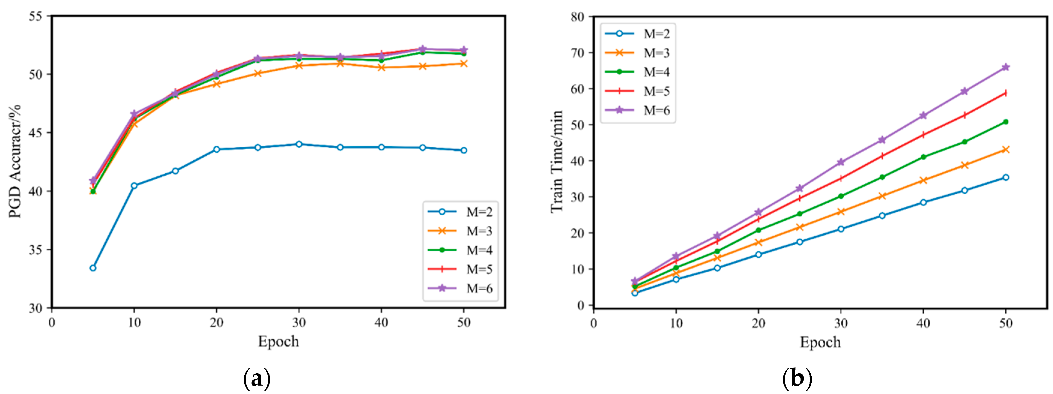
This paper experiments with five different cases by setting , , , , and , while keeping the training step size . Each case is subjected to 10 independent rounds of adversarial training with a gap of 5 rounds between 5 and 50 rounds, and the training time is recorded. Then, the models trained under each case are evaluated using PGD-20 adversarial attacks, and the results are recorded. The specific experimental results are shown in Figure 2.
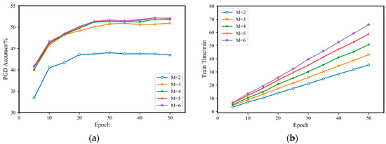
Figure 2.
Comparison of Fast-M adversarial training on CIFAR10 with different iteration stage numbers M: (a) accuracy for a PGD-20 attack; (b) training time.
From Figure 2b, it can be observed that with the increase in training rounds, the difference in training time between different values of gradually increases, which is consistent with the theoretical data in Table 1. Moreover, from Figure 2a, the model’s accuracy gradually improves with increasing . When , the accuracy of the adversarial training model for PGD-20 reaches a large and stable value. As continues to increase, the accuracy only slightly increases, while the training time increases significantly. Therefore, on the CIFAR10 dataset, selecting to be 4 or 5 is appropriate.
6.2.2. Training Step Size Selection
The effect of the training step size on fast adversarial training was discussed above. However, since Fast-M has internal iterations, a smaller training step size may lead to the phenomenon of “catastrophic overfitting”. Therefore, in this paper, different training step sizes were compared under the parameters of and . The training step size was varied from 1/255 to 16/255, and the experimental results are shown in Figure 3.
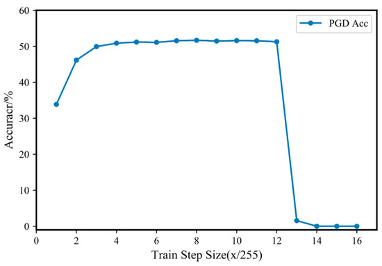
Figure 3.
PGD attack accuracy of Fast-5 adversarial training with different training step sizes on CIFAR10.
Figure 3 shows the PGD attack accuracy of Fast-5 adversarial training on the CIAFR10 dataset under different training step sizes. It can be seen from the figure that Fast-M adversarial training can also experience “catastrophic overfitting”. However, a smaller training step size can also achieve good training results. When is between 4/255 and 12/255, the accuracy of the trained model for the PGD-20 attack is stable. The maximum accuracy is achieved when . Therefore, the most appropriate choice for the training step size on the CIAFR10 dataset is approximately 8/255, which is consistent with the perturbation limit range .
6.2.3. Evaluation Comparison of Fast-M Adversarial Training
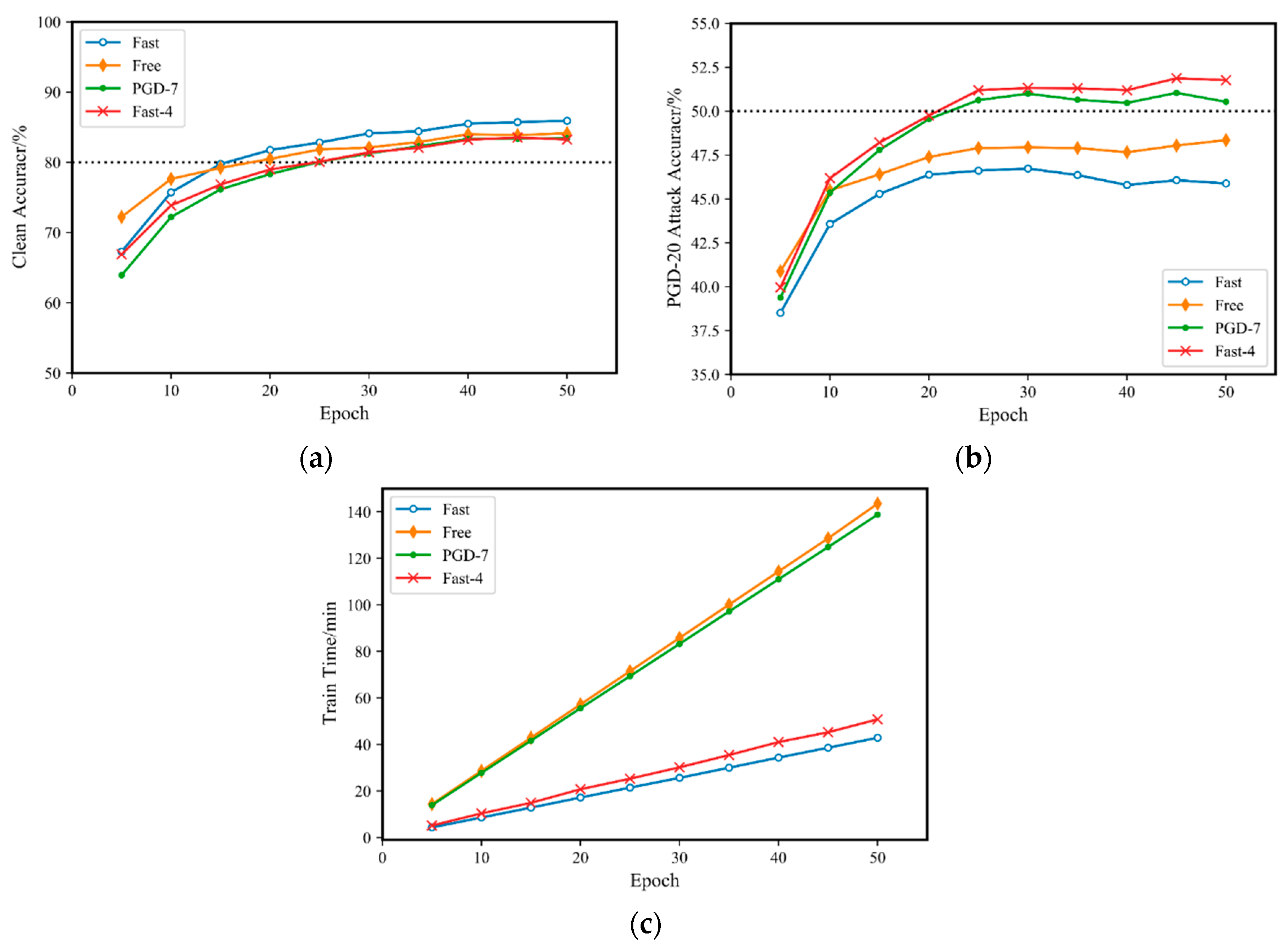
To demonstrate the effectiveness of the Fast-M adversarial training method, this paper compares it with three other adversarial training methods: fast adversarial training (, ), free adversarial training (, ), and PGD adversarial training (, , ). The Fast-M method used in this paper takes , , and . The training starts from , with one model trained every five epochs, until . Ten different neural network models are trained independently, and the training time is recorded. Then, the trained models are tested for their accuracy based on the original clean samples and on the samples for the PGD-20 () attack. The results are shown in Figure 4.
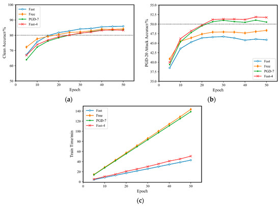
Figure 4.
Comparison of Fast-M adversarial training and multiple adversarial training methods on CIAFR10: (a) accuracy for the original clean sample; (b) accuracy for a PGD-20 attack; (c) training time.
As shown in Figure 4b, both Fast-4 adversarial training and PGD-7 adversarial training achieved an accuracy of over 50% for the PGD-20 attack. Moreover, the accuracy of Fast-4 adversarial training was slightly higher than that of PGD-7 adversarial training. On the other hand, the accuracies of free adversarial training and fast adversarial training for the PGD-20 attack were both approximately 47%. It is also clear that the accuracy of fast adversarial training for the PGD-20 attack did not exceed 50%, even as the number of training rounds was increased, and remained at approximately 46%. In contrast, Fast-4 adversarial training and PGD-7 adversarial training under the same number of training rounds easily achieved 50% accuracy under the same attack.
As shown in Figure 4a,b, although fast adversarial training does not perform well for PGD-20 adversarial attacks, its evaluation accuracy for the original clean samples is similar to that of the other three adversarial training methods. However, its advantage is not significant, achieving an accuracy of approximately 85%, while the other three methods achieve an accuracy of 83%. The gap in accuracy between the original clean samples and PGD adversarial samples is relatively small, indicating a balance between the two. In adversarial training, neural networks are trained to simultaneously handle adversarial examples and clean examples. By minimizing the loss of adversarial examples, the network learns the features of adversarial examples to more accurately identify and classify them. However, during the adversarial training process, if not properly constrained, the neural network model may overly focus on adversarial examples. This excessive attention can lead to a decrease in classification accuracy when dealing with clean examples. Because the network learns how to differentiate adversarial examples, it may overfit the features of adversarial examples and overlook the characteristics of clean examples.
As shown in Figure 4c, the training times of Fast-4 adversarial training and fast adversarial training are much less than those of PGD-7 and free adversarial training () under the same number of training rounds. Furthermore, the training time of Fast-4 adversarial training is only slightly higher than that of fast adversarial training, is still within the same range, and does not increase significantly. It is worth noting that free adversarial training cannot benefit from cyclic learning as PGD adversarial training does, so its training time is similar to that of PGD-7 adversarial training in the case of m = 8.
Therefore, based on the experimental results in Figure 4, the proposed Fast-M algorithm is very effective. It improves the accuracy of fast adversarial training for PGD adversarial attacks by over 5% while ensuring that the training time does not increase significantly. Moreover, the accuracy after improvement is slightly higher than that of traditional PGD-7 adversarial training.
To further demonstrate the effectiveness of the Fast-M adversarial training algorithm, it is compared with various existing adversarial training algorithms under different parameter settings. The comparison results are shown in Table 2.
Table 2.
Comparison of various adversarial training algorithms on the CIFAR10 dataset after 30 rounds of training.
From the data in Figure 4, all the compared adversarial training algorithms reach a stable accuracy for PGD adversarial attacks after 30 rounds of training and no longer have significant changes. Therefore, all algorithms in this comparison experiment were trained for 30 rounds, and their training times were recorded for comparison.
The algorithms compared in this experiment include fast, free (), free (), PGD-7, PGD-10, Amata (,), and the proposed Fast-3, Fast-4, and Fast-5. In addition to comparing training time, different perturbation ranges and different numbers of iterations of PGD adversarial attacks were also added as further evaluation methods. From the data shown in Table 2, the Fast-M adversarial training algorithm not only has a significant advantage in training time but also has better accuracy than other compared adversarial training algorithms under various attack methods, which sufficiently proves the effectiveness of the Fast-M adversarial training algorithm.
6.3. Verification of Fast-M on CIFAR100
In order to further verify the validity of the Fast-M method, we utilized the more complex PreActResNet34 architecture on the CIFAR100 dataset, which contains images with more diverse content. The experimental results, as shown in the Table 3, reveal that under PGD adversarial attacks on a more intricate dataset and network structure, the original Fast method exhibited minimal defensive capabilities. Conversely, our proposed Fast-M method demonstrated defense capabilities comparable to PGD adversarial training. Specifically, when M = 5, the results indicate superior performance on both clean test data and under PGD-20 and PGD-50 adversarial attacks compared to PGD adversarial training. Notably, the training time required is less than one-third of PGD-10, further validating that our Fast-M adversarial training method achieves results akin to PGD adversarial training at a significantly reduced training cost and in some cases surpasses it.
Table 3.
Comparison of various adversarial training algorithms on the CIFAR100 dataset using PreActResNet34 after 100 epochs of training.
7. Conclusions
This paper proposes an improved Fast-M adversarial training algorithm based on the fast adversarial training method. The Fast-M adversarial training algorithm presented in this article can train a more robust neural network model in the same training time as the fast adversarial training method. The model’s classification accuracy for PGD adversarial attacks can reach the same level as a neural network model trained for more time using PGD adversarial training or even slightly surpass it. Additionally, extensive comparative experiments on the MNIST, CIFAR10, and CIFAR100 datasets were conducted. The experimental results fully validate the effectiveness of the proposed method. However, compared to PGD adversarial training, it does not show a significant improvement. This may be due to the limitations imposed by the conventional FGSM adversarial perturbation. Using FGSM adversarial perturbation for adversarial training does not yield a noticeable defense effect against PGD adversarial attacks. Future research should focus on obtaining stronger adversarial samples for adversarial training without significantly increasing the required training time. Additionally, we intend to explore the utilization of approximation methods and precomputing techniques to mitigate the computational complexity associated with our proposed approach. One potential avenue involves precomputing a set of adversarial samples and reusing them during the training process, thereby further reducing the training costs. We firmly believe that this research direction holds promise in enhancing the practicality and efficiency of our method. We look forward to making significant strides in this direction, striking a better balance between the computational efficiency of adversarial training and the robustness of the trained models, thereby advancing the practical application of adversarial training.
Author Contributions
Conceptualization, Y.M., D.A. and Z.G.; methodology, Y.M., D.A. and Z.G.; software, Z.G.; validation, Y.M. and Z.G.; formal analysis, Z.G.; investigation, D.A. and Z.G.; resources, D.A.; data curation, Z.G.; writing—original draft preparation, Y.M. and Z.G.; writing—review and editing, Y.M., D.A. and Z.G.; visualization, Z.G.; supervision, D.A. and J.L.; project administration, D.A. and J.L.; funding acquisition, Y.M., D.A. and W.L. All authors have read and agreed to the published version of the manuscript.
Funding
This research was funded by the National Natural Science Foundation of China under Grant 62173268, the National Postdoctoral Innovative Talents Support Program of China under Grant BX20200272, the Natural Science Basic Research Program of Shaanxi under Grant 2021JQ-288, and the Fundamental Research Funds for the Central Universities, CHD under Grant 300102320101.
Institutional Review Board Statement
Not applicable.
Informed Consent Statement
Not applicable.
Data Availability Statement
The original contributions presented in this study are included in the article; further inquiries can be directed to the corresponding author.
Conflicts of Interest
The authors declare no conflicts of interest.
References
- Akhtar, N.; Mian, A. Threat of adversarial attacks on deep learning in computer vision: A survey. IEEE Access 2018, 6, 14410–14430. [Google Scholar] [CrossRef]
- Szegedy, C.; Zaremba, W.; Sutskever, I.; Bruna, J.; Erhan, D.; Goodfellow, I.; Fergus, R. Intriguing properties of neural networks. arXiv 2013, arXiv:1312.6199. [Google Scholar]
- Goodfellow, I.J.; Shlens, J.; Szegedy, C. Explaining and harnessing adversarial examples. In Proceedings of the International Conference on Learning Representations, Banff, AB, Canada, 14–16 April 2014; Volume 101. [Google Scholar]
- Wong, E.; Rice, L.; Kolter, J.Z. Fast is better than free: Revisiting adversarial training. In Proceedings of the International Conference on Learning Representations, New Orleans, LA, USA, 6–9 May 2019; Volume 103. [Google Scholar]
- Papernot, N.; McDaniel, P.; Wu, X.; Jha, S.; Swami, A. Distillation as a defense to adversarial perturbations against deep neural networks. In Proceedings of the 2016 IEEE Symposium on Security and Privacy (SP), San Jose, CA, USA, 22–26 May 2016; pp. 582–597. [Google Scholar]
- Metzen, J.H.; Genewein, T.; Fischer, V.; Bischoff, B. On detecting adversarial perturbations. In Proceedings of the International Conference on Learning Representations, Toulon, France, 24–26 April 2017. [Google Scholar]
- Feinman, R.; Curtin, R.R.; Shintre, S.; Gardner, A.B. Detecting adversarial samples from artifacts. arXiv 2017, arXiv:1703.00410. [Google Scholar]
- Pinot, R.; Ettedgui, R.; Rizk, G.; Chevaleyre, Y.; Atif, J. Randomization matters how to defend against strong adversarial attacks. In Proceedings of the 37th International Conference on Machine Learning, PMLR, Virtual Event, 13–18 July 2020; pp. 7717–7772. [Google Scholar]
- Madry, A.; Makelov, A.; Schmidt, L.; Tsipras, D.; Vladu, A. Towards deep learning models resistant to adversarial attacks. In Proceedings of the International Conference on Learning Representations, Vancouver, BC, Canada, 30 April–3 May 2018; Volume 97. [Google Scholar]
- Shafahi, A.; Najibi, M.; Ghiasi, M.A.; Xu, Z.; Dickerson, J.; Studer, C.; Davis, L.S.; Taylor, G.; Goldstein, T. Adversarial training for free! In Proceedings of the Advances in Neural Information Processing Systems, Vancouver, BC, Canada, 8–14 December 2019; Volume 32.
- Smith, L.N.; Topin, N. Super-convergence: Very fast training of neural networks using large learning rates. In Proceedings of the Artificial Intelligence and Machine Learning for Multi-Domain Operations Applications, SPIE, Baltimore, MD, USA, 14–18 April 2019; Volume 11006, pp. 369–386. [Google Scholar]
- Micikevicius, P.; Narang, S.; Alben, J.; Diamos, G.; Elsen, E.; Garcia, D.; Ginsburg, B.; Houston, M.; Kuchaiev, O.; Venkatesh, G.; et al. Mixed precision training. In Proceedings of the International Conference on Learning Representations, Vancouver, BC, Canada, 30 April–3 May 2018; Volume 95. [Google Scholar]
- Ye, N.; Li, Q.; Zhou, X.Y.; Zhu, Z. Amata: An annealing mechanism for adversarial training acceleration. In Proceedings of the AAAI Conference on Artificial Intelligence, Vancouver, BC, Canada, 2–9 February 2021; Volume 35, No. 12. pp. 10691–10699. [Google Scholar]
- Sriramanan, G.; Addepalli, S.; Baburaj, A. Guided adversarial attack for evaluating and enhancing adversarial defenses. In Proceedings of the Advances in Neural Information Processing Systems, Virtual, 6–12 December 2020; Volume 33, pp. 20297–20308. [Google Scholar]
- Kurakin, A.; Goodfellow, I.J.; Bengio, S. Adversarial examples in the physical world. In Artificial Intelligence Safety and Security; Chapman and Hall/CRC: Boca Raton, FL, USA, 2018; pp. 99–112. [Google Scholar]
- Moosavi-Dezfooli, S.M.; Fawzi, A.; Frossard, P. Deepfool: A simple and accurate method to fool deep neural networks. In Proceedings of the IEEE Conference on Computer Vision and Pattern Recognition, Las Vegas, NV, USA, 27–30 June 2016; pp. 2574–2582. [Google Scholar]
- Carlini, N.; Wagner, D. Towards evaluating the robustness of neural networks. In Proceedings of the 2017 IEEE Symposium on Security and Privacy (SP), San Jose, CA, USA, 22–24 May 2017; pp. 39–57. [Google Scholar]
- Su, J.; Vargas, D.V.; Sakurai, K. One pixel attack for fooling deep neural networks. IEEE Trans. Evol. Comput. 2019, 23, 828–841. [Google Scholar] [CrossRef]
- Papernot, N.; McDaniel, P.; Goodfellow, I.; Jha, S.; Celik, Z.B.; Swami, A. Practical black-box attacks against deep learning systems using adversarial examples. arXiv arXiv:1602.02697, 2016.
- Chen, P.Y.; Zhang, H.; Sharma, Y.; Yi, J.; Hsieh, C.J. Zoo: Zeroth order optimization based black-box attacks to deep neural networks without training substitute models. In Proceedings of the 10th ACM Workshop on Artificial Intelligence and Security, Dallas, TX, USA, 3 November 2017; pp. 15–26. [Google Scholar]

Disclaimer/Publisher’s Note: The statements, opinions and data contained in all publications are solely those of the individual author(s) and contributor(s) and not of MDPI and/or the editor(s). MDPI and/or the editor(s) disclaim responsibility for any injury to people or property resulting from any ideas, methods, instructions or products referred to in the content. |
© 2024 by the authors. Licensee MDPI, Basel, Switzerland. This article is an open access article distributed under the terms and conditions of the Creative Commons Attribution (CC BY) license (https://creativecommons.org/licenses/by/4.0/).