Abstract
As an advanced detection technique, electrical resistive tomography (ERT) has been applied to detect the solid–liquid two-phase flow velocity based on available ERT measurements. The flow velocity computation by ERT must depend on the relative algorithms, including both the cross-correlation (CC) principle and convolutional neural networks (CNNs). However, these two types of algorithms have poor accuracy and generalization under complex measuring conditions and various flow patterns. To address this issue, in this paper, a hybrid network is proposed that combines a CNN with a reproducing kernel-based support vector machine (RKSVM) technique. The features hidden in ERT measurements are extracted using the CNN, and then the flow velocity is computed by the RKSVM in a high-dimensional feature space. According to the ERT measurements in an actual experimental platform, the results show that the hybrid network has higher accuracy and generalization ability for flow velocity computation compared with the existing CC, RKSVM, and CNN methods.
1. Introduction
Flow velocity is an important parameter for multiphase flow detection [1,2]. As an advanced detection technique, electrical resistive tomography (ERT) [3] has real-time, noninvasive, fast response advantages and is widely utilized in industrial detection [4,5]. The flow velocity computation performed by ERT must depend on the relative algorithms, the most typical of which include both the cross-correlation (CC) [6] principle and convolutional neural networks (CNNs) [7].
In the past decade, various methods for flow velocity computation have been presented based on the CC principle under available ERT measurements. The CC-based methods compare two groups of correlative measuring series obtained by two adjacent ERT sensors. Then, the flow velocity can be computed from the crossing time and distance between the two adjacent ERT sensors. However, in most cases, these CC methods remain inaccurate due to the following three problems: unreasonable “frozen” assumption in CC [7], natural ERT limitations [8], and uncertain length of comparing series [9]; however, some progress has been made [10,11].
In recent years, CNNs have been applied to flow velocity detection. The flow velocity prediction model [12] was established based on a deep neural network, which could take advantage of CNNs and Bi-LSTMs to extract features in time series and be combined with a self-attention mechanism to improve prediction performance. In the same direction, two different models based on the CNN and the encoder–decoder method were established to predict the characteristics of the flow velocity and heat transfer around the NACA sections [13]. Essentially, some research groups designed various CNNs to perform flow velocity computation [14]. For example, Liu et al. [15] used the CNN to calculate flow velocity owing to the generalization and feature extraction ability, while the transfer learning method can train the network in advance. More reviews can be found in [16]. Despite progress, these existing CNN-based methods have their individual limitations. First, due to the black-box state of the deep learning process, the generalization of CNNs is unclear and incomprehensive. Second, the computed accuracy of CNNs is often too unstable to satisfy the requirement of flow velocity detection when the flow velocity changes quickly. These problems limit the applicable range of CNNs in applications.
To address the above problems, we propose a method for flow velocity detection along the existing least square-based support vector machine (LS-SVM) algorithm. LS-SVM is an improved support vector machine (SVM) method proposed by Suykens et al. [17] that is widely used in pattern recognition and nonlinear regression due to its simplified computational complexity. LS-SVM uses a reproducing kernel function to map the input to a high-dimensional feature space, which can effectively enhance the generalization of SVM prediction. According to the LS-SVM algorithm, in this paper, we design a hybrid network which combines a CNN with a reproducing kernel-based support vector machine (RKSVM) technique. Firstly, the features hidden in ERT measurements are extracted using the CNN, and then the feature data are mapped to a high-dimensional feature space by a selected reproducing kernel function. Finally, the flow velocity is generally computed by the hybrid network in a high-dimensional feature space. The proposed method is expected to have stronger generalization capabilities and greater accuracy than the typical CC, RKSVM, and CNN methods.
2. Related Work
2.1. Cross-Correlation Principle
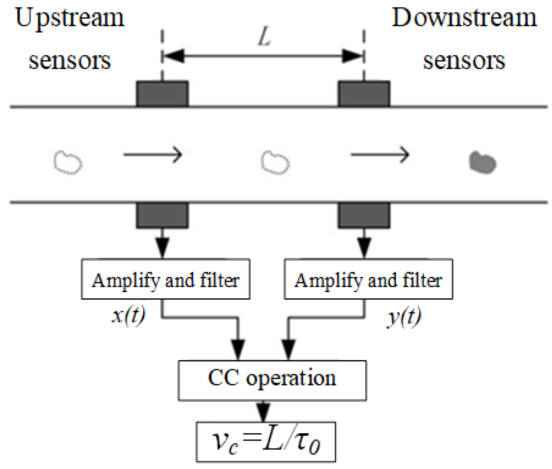
The cross-correlation (CC) computation results from the principle of stochastic processes and analysis of random signals [18]. The CC method compares two groups of correlative measuring series obtained by two adjacent ERT sensors, i.e., an upstream sensor x(t) and a downstream sensor y(t) along the flow direction, as shown in Figure 1. Both the upstream sensor and the downstream sensor are parallelly mounted on the pipe.
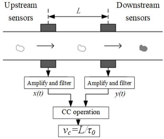
Figure 1.
Schematic diagram of CC principle.
If the fluid in the pipe conforms to the “freezing” assumption [19], the ERT measuring series between the two sensors will be sufficiently similar. Hence, the transit time τ between the two sensors can be measured when the distance between them is L. The flow velocity can be computed as
However, the “freezing” assumption is not true in most cases that have complex flow patterns and various measuring conditions in dredging engineering [20]. The noise in the ERT measurement can greatly affect the accuracy of the CC method. The complementarity between similarity norms in the CC method is seldom used. In addition, the CC method cannot determine the optimal series length, which can greatly affect the accuracy of the CC estimation. Therefore, the accuracy of the computational flow velocity by the CC principle and ERT measurements cannot be guaranteed.
2.2. Convolutional Neural Network
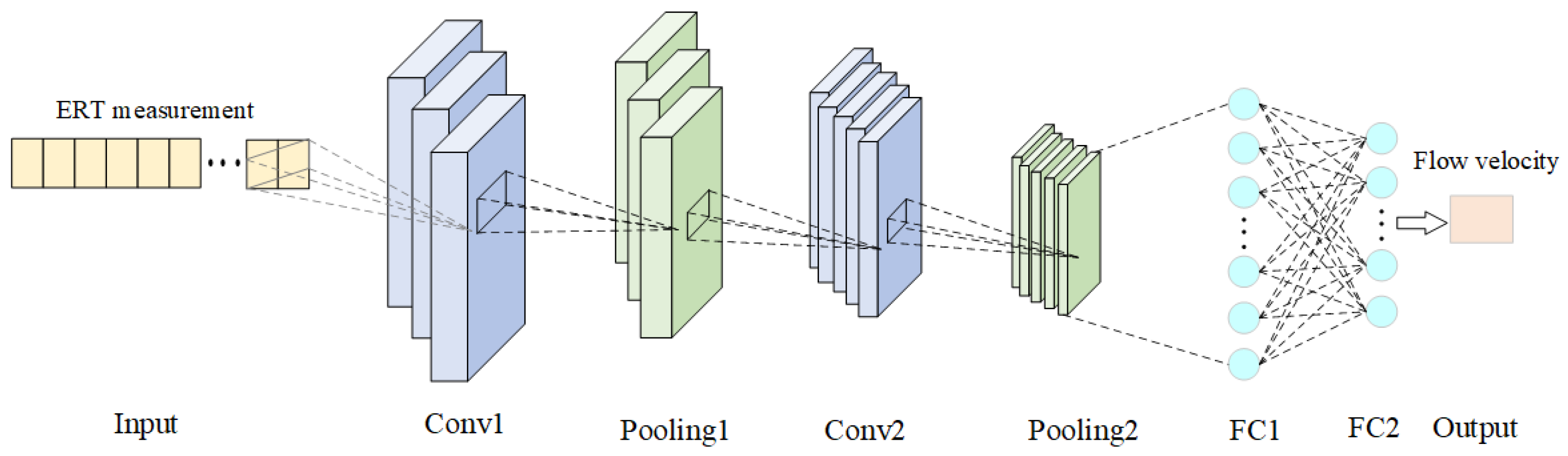
The convolutional neural network (CNN) is a deep feedforward neural network based on the idea of local connectivity and parameter sharing [21]. The structure of a typical CNN for flow velocity prediction is shown in Figure 2.

Figure 2.
The structure of a typical CNN for flow velocity prediction.
The CNN generally consists of multiple convolutional layers and pooling layers. The convolutional layer effectively captures feature data by applying a series of filters or convolution kernels to the input data. Moreover, the convolutional kernel computes only local information from the input data at a single point in time, which allows the CNN to better extract the deep features. The pooling layer is used for the secondary extraction of features obtained from the convolutional layer in order to reduce the feature dimensions, and common pooling operators include maximum pooling, average pooling, and sum pooling. The two FC layers of FC1 and FC2 convert the extracted features into a one-dimensional (1D) matrix for feature combinations and transformations, and FC2 decreases the connection of the CNN in the FC layer to a low dimension (e.g., 10 dimensions in this paper). These are ultimately passed on to the output layer to obtain the results.
2.3. Reproducing Kernel Function
Let H be a Hilbert function space, and each function is defined on a set of D. For any two functions of u and v ∈ H, their inner product is represented as
For any , if a function ∈H satisfies , H is called a reproducing kernel space, and is the reproducing kernel function on H [22].
A Sobolev Hilbert space on is composed of all continuous complex functions and has a finite number of paradigms.
where a and c > 0. The reproducing kernel of a Sobolev Hilbert space can be expressed as
The translation invariant kernel function can be obtained from Equation (4) as
This can be proved by the Fourier variation of Equation (4),
Similarly, it can be proved by Equation (5),
From Equations (6) and (7), the Equation (3) translation invariant kernel function satisfies the Mercer condition for the SVM kernel function [23].
2.4. Reproducing Kernel-Based Support Vector Machine
The reproducing kernel-based support vector machine (RKSVM) [24] is an improvement on the typical SVM based on the reproducing kernel function of Equation (5).
If is the sample vector in a d-dimensional space and is the label of the sample, , then the dataset of all samples can be represented as , where and , and n is the total number of samples.
RKSVM transforms any sample data in to a high-dimensional feature space by a nonlinear mapping , and the linear regression model for a dataset of all samples is constructed in the high-dimensional feature space as
where is the multiplier of support vectors, and b is the parametrized vector.
The optimization problem for the above regression model is
where is the regularization parameter, is the slack variable, and e is a unit vector.
The Lagrange function is defined using Equation (9) as follows,
where is the vector on the Lagrange multiplier. Let these partial derivatives of L for , , , and equal 0. Then, the above optimization problem is used to solve the following equation group,
where , and thus, the following equation is obtained from Equation (11):
Let the kernel function be , where is the reproducing kernel function of Equation (5). Equation (12) is simply the regress function of RKSVM, which can be rewritten as
where is a positive definite matrix, and is solved by Equation (11).
Compared with the typical SVM, the RKSVM has three advantages. First, the matrix in RKSVM is positive and definite, and then the optimization process is performed once to solve the RKSVM model rather than multiple iterative optimizations, which is the case with the SVM. Second, without the need to solve for b, the RKSVM reduces the number of solved variables by half compared to that of the SVM. Finally, the linear regression in RKSVM has stronger generalization capabilities than those in the SVM. Hence, our design starts from RKSVM in this paper.
3. The Hybrid Network for Flow Velocity Computation
3.1. Structure of Hybrid Network
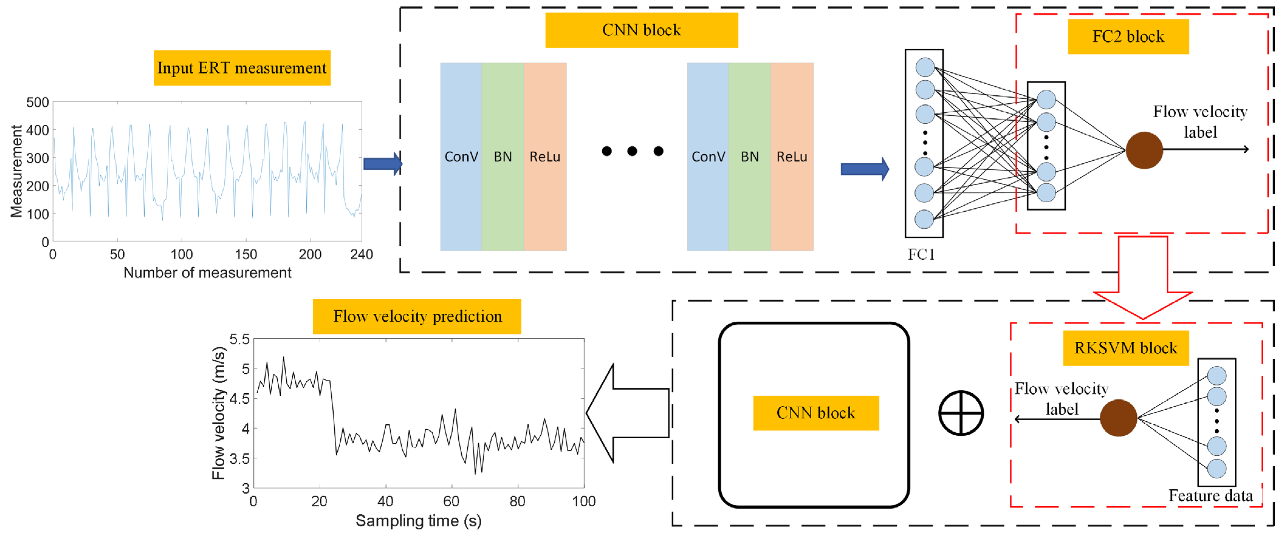
Because of the advantages of the CNN and the RKSVM, we proposed a hybrid network based on the CNN and the RKSVM (CNN–RKSVM), as shown in Figure 3. The CNN–RKSVM consists of a CNN block, an FC block, and an RKSVM block, in which the structure of the CNN block and FC block in the hybrid network is adapted from the AlexNet network [25]. The network training process of the CNN–RKSVM comprises two stages as follows.
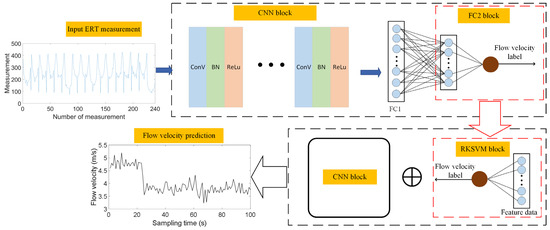
Figure 3.
Structure of the proposed hybrid network.
In the first stage, the CNN block extracts the key features from input ERT measurements through the convolutional layer. In addition, the batch normalization (BN) layer and the rectified linear unit (ReLu) activation function are behind the convolutional layer. The BN layer is used to normalize the output from the convolutional layer to improve the generalization ability of the used network, and the ReLu activation function is used to improve the feature extraction and the network performance. In the convolutional layer, the same padding is chosen on the input ERT measurements to ensure that the input and output of the convolutional layer have the same size. The amount of padding is determined based on the size of the convolution kernel and the step size. In this way, the loss of information at the boundaries of the input data can be avoided, and it also helps to improve the performance and stability of the proposed network.
The second stage starts from the training results in the first stage, where the FC2 block generates a set whose element is formulized as (w1(t), w2(t), …., w10(t), v(t)). In this set, t denotes the tth iteration, and v(t) is the sample label of flow velocity at total T iterations, where t = 1, 2, …, T. The FC2 block is transformed to the set of the RKSVM block, and the set of {(w1(t), w2(t), …., w10(t), v(t)) t = 1, 2, …, T} is used to train the RKSVM block. Finally, the completed RKSVM is taken back into the CNN block and replaces the FC2 layer as the output of the CNN block, and the integration of the CNN and the RKSVM is shown by the sign “⊕”. Consequently, the learning process completed the network, and the trained hybrid network termed CNN–RKSVM can predict and compute the flow velocity.
In regular CNN-based models, a small convolutional kernel is usually chosen. A large number of researchers have followed this guideline of using small convolutional kernels when designing models, and few have used large convolutional kernels. However, the ERT measurements are the 1D data; thus, the network parameters, such as the number of convolutional and pooling layers, the kernel size, and the step size, are determined based on the quality of features extracted by the CNN block. The structure of the CNN block and the FC block is shown in Table 1.

Table 1.
The structure of the CNN block and FC block.
3.2. Training of CNN–RKSVM
During the process of network training, in the CNN block in the first stage, the ERT measurements are used as inputs, the real flow velocities are used as outputs (labels), and the parameters of the CNN block are determined by minimizing the following loss function:
where N is the number of the sample dataset, is the ith real flow velocity, is the ith predicted flow velocity, θ represents the parameters of the CNN block, and is a hyperparameter that is used to balance the effect between the two terms. In this paper, the value of is taken as 10−3 after a larger number of comparable performances.
In the second stage, the feature data extracted from the CNN block and FC block are used as inputs in the RKSVM block. The loss function is Equation (9), and the optimal parameters of the RKSVM are determined by minimizing Equation (9).
The CNN–RKSVM in this paper was trained on a server with a Windows 10 (64-bit) operating system with the following hardware configuration parameters: CPU processor Intel(R) Core (TM) i7-9800X, 3.80 GHz; 64 GB of operating memory; and dual NVIDIA GeForce RTX 2080Ti 11 GB graphics cards. During the network training process of the CNN–RKSVM parameters, the adaptive moment estimation (Adam) algorithm [26] updates the parameters θ. The initialization parameters for the hybrid network are often empirically determined during training. The initial learning rate is set to 0.001, the attenuation coefficient is 0.1, the regularization factor is 0.0001, and the learning rate decay is 0.5. The network is trained for 200 epochs with a batch size of 128.
3.3. The Sample Dataset
The sample dataset consists of ERT measurements and the corresponding real flow velocities, which were obtained from the Tianjin Dredging Co., Ltd., Tianjin, China. The ERT measurements are obtained by the ERT system, and the real flow velocities are obtained by the electromagnetic flowmeter. Moreover, the ERT system in this paper used the single electrode measurement after single electrode excitation. Thus, for the 16-electrode ERT system, 240 measurements can be obtained as the input of the CNN–RKSVM.
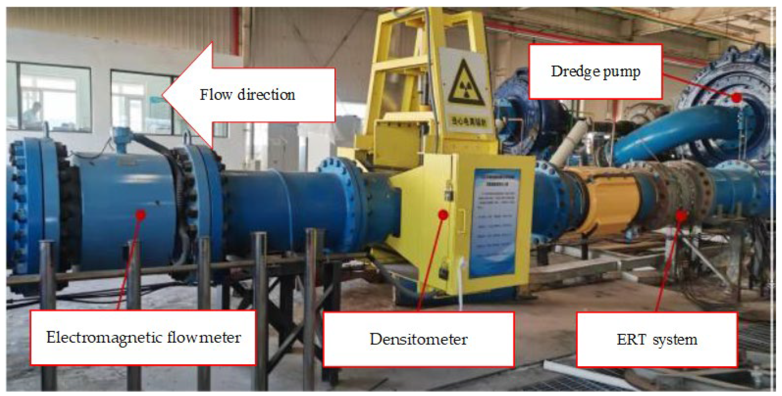
The pipeline of the dredging transportation experimental platform has a diameter of 0.8 m and a length of 358 m. The horizontal pipe section is installed with measuring devices such as an electromagnetic flowmeter, a densitometer, and an ERT system. The flow direction of solid–liquid two-phase flow is shown in Figure 4. The distance between the electromagnetic flowmeter and the ERT system is 5 m. The difference in flow velocity between the two locations of the electromagnetic flowmeter and the ERT system is negligible under the experimentally set working conditions. In addition, the distance between the two adjacent ERT sensors is 0.3 m.

Figure 4.
Dredging engineering experimental platform.
As shown in Figure 4, the solid phase and liquid phase were mixed into a solid–liquid two-phase flow in a mixing tank, which was further transferred into a transporting pipeline by the dredge pump. The solid phase included coarse sand and gravel (with a conductivity of approximately 0 mS/cm). Different types of solid-phase objects were employed to evaluate the applicability of various methods for flow velocity along different flow patterns. Meanwhile, the liquid phase consisted of water (with a conductivity of 1.3 mS/cm). The flow velocities and solid phase fractions (SPFs) were adjustable by means of a dredge pump in the pipeline. The inlet solid–liquid two-phase flow velocity was 1–6 m/s, and the SPF ranged between 5% and 40%.
The accuracy and generalization of the CNN–RKSVM are strongly dependent on the quality of the sample dataset. Therefore, simulating actual working conditions is crucial for obtaining ERT measurements under different SPFs and flow velocities.
The solid phase used in the experiments included coarse sand and gravel. For coarse sand, the experiments involved eight SPFs: 5%, 10%, 15%, 20%, 25%, 30%, 35%, and 40%. For gravel, the experiments involved six SPFs: 5%, 10%, 15%, 20%, 25%, and 30%. The flow velocity ranged from 0 m/s to 6 m/s for both types of solid phases under different SPFs. To enhance the generalization ability of the CNN–RKSVM, ERT measurements from two types of solid-phase objects were combined to form the sample dataset. The sample dataset was grouped to training and testing datasets according to the 10-fold cross-validation method. The data distribution of the datasets and their sample sizes are shown in Table 2.
Table 2.
Distribution of sample dataset.
4. Experimental Results and Discussion
4.1. Evaluation Parameters
The CNN–RKSVM method is quantitatively assessed using three evaluation metrics: the root mean square error (RMSE), the mean absolute percentage error (MAPE), and runtime compared with existing flow velocity detection methods. The RMSE and MAPE describe the error between the real flow velocity and the predicted flow velocity. The runtime describes the time taken to obtain a frame of predicted flow velocity.
RMSE is defined as
where is the real flow velocity from the electromagnetic flowmeter, is the predicted flow velocity from any of the methods, and i is the ith sampling. The RMSE quantifies the disparity between real flow velocity and predicted flow velocity. A smaller RMSE indicates a more accurate prediction, whereas a larger RMSE signifies a greater prediction error and decreased model efficacy.
MAPE is defined as
MAPE indicates the deviation degree between the predicted flow velocity calculated using the testing method and the real flow velocity; the closer MAPE is to 0, the more accurate the model.
4.2. Results and Discussion
Based on the above sample dataset, the flow velocities of the test dataset obtained by the CNN–RKSVM are compared with the CC, RKSVM, and CNN methods.
The solid–liquid two-phase flow within dredging engineering has a critical flow velocity (V0), and in this experiment, V0 is nearly 2.3 m/s. When the flow velocity is greater than V0, the solid phase inside the pipe is in a suspended state, and the flow pattern is under turbulent flow. Conversely, when the flow velocity is less than V0, the solid phase inside the pipe settles at the bottom of the pipe, and the flow pattern is under laminar flow. Therefore, in order to compare these two flow velocity cases, the results of flow velocity are divided into two groups: low flow velocity and high flow velocity, as shown in Figure 5.
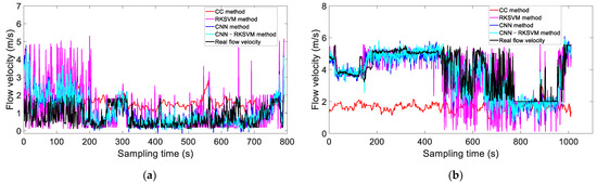
Figure 5.
Comparison of flow velocities for four methods. (a) V < V0. (b) V > V0.
Figure 5a shows that when the flow velocity is smaller than V0, the flow velocity obtained by the CC method exhibits a similar trend to the real flow velocity, albeit with a larger error compared to the CNN and CNN–RKSVM methods. In contrast, the RKSVM ha some errors with the real flow velocity. Compared with the CNN, the computed flow velocities from the CNN–RKSVM are very close to the real flow velocities. The CNN–RKSVM uses the RKSVM to map the feature data extracted from the CNN into the high-dimensional space to obtain the flow velocities so that the flow velocities obtained by the CNN–RKSVM are very close to the real flow velocities.
Figure 5b shows that when the flow velocity exceeds V0, the CC method fails to accurately capture the flow velocity due to the non-fulfillment of the “freezing” model. Particularly, when the flow velocity surpasses 4 m/s, the solid phase within the pipeline exhibits a uniform distribution, resulting in a high similarity of ERT measurements. The RKSVM and CNN methods show some deviation from the real flow velocity, whereas the CNN–RKSVM provides a closer approximation.
To quantitatively evaluate the CNN–RKSVM, we compared it with the CC, RKSCN, and CNN methods. The RMSEs, MAPEs, and runtimes for the four methods of calculating flow velocity are compared with those of real flow velocity, as shown in Table 3.
Table 3.
Evaluation parameters for the four methods.
Table 3 shows that the RMSEs of the CC method are always greater than 0.8 and that the MAPEs of the CC method are greater than 0.2. The RKSVM method is relatively stable regardless of whether V > V0 or V < V0, but it may lead to a large error with partial testing samples. Owing to the advantage of deep learning in both the CNN and CNN–RKSVM methods, their RMSEs and MAPEs are much smaller than those of the CC and RKSVM methods. Both the CNN and CNN–RKSVM methods yield a more consistent flow velocity when the flow velocity is less than V0. However, when the flow velocity is greater than V0, the RMSE and MAPE of the CNN–RKSVM method are better than those of the CNN method. Since the RKSVM uses the reproducing kernel as the kernel function, it has advantages, including a strong generalization ability and a high computational efficiency. Therefore, the CNN–RKSVM based on both the RKSVM and the CNN can improve the accuracy, generalization ability, and robustness of flow velocity calculations.
Moreover, the CNN–RKSVM method uses reproducing kernel functions to avoid the computation of inner products in high-dimensional spaces and thus greatly reduces the computational load and shortens the model computation time under the learning process. On the other hand, the bottom line in Table 3 shows the runtimes of the four methods, CC, RKSVM, CNN, and CNN–RKSVM, at any new ERT measurements. It is clear that the CNN–RKSVM has the longest time cost while the CC has the lowest since the CNN–RKSVM must use more blocks and parameters to compute flow velocity. Nevertheless, the runtimes of the CNN–RKSVM are less than 1 s, which is an acceptable response time in dredging engineering.
5. Conclusions
Flow velocity detection plays an increasingly important role in dredging engineering. In this paper, a method combining a CNN and a RKSVM was used to calculate the flow velocity. The proposed method was designed in two stages. In the first stage, the ERT measurements of different types of solid phases, various SPFs, and distinct flow velocities were obtained from the dredging engineering experimental platform, which constituted the sample dataset. Then, the feature data of the sample dataset were extracted through the CNN block. Accordingly, the feature data were transformed to the FC block and consisted of a new learning dataset for the second stage. In the second stage, the RKSVM was built by the new learning dataset. After the RKSVM was trained well, it replaced the FC block in the CNN block in the first stage. Consequently, the CNN–RKSVM was created for the flow velocity calculation. Our experiments showed that the CNN–RKSVM method overcame problems such as low accuracy and poor generalization compared to existing flow velocity detection methods. Therefore, the CNN–RKSVM method proposed in this paper provides a new method for flow velocity detection in dredging engineering.
However, the sample dataset used in this paper was obtained by the Tianjin Dredging Co., Ltd., and parameters such as viscosity coefficient and conductivity of the solid–liquid two-phase flow were fixed. Therefore, the sample dataset did not contain all the working conditions in dredging engineering. In addition, the input of the CNN–RKSVM method was the 1D ERT measurements, which lose some of the neighborhood information during the feature extraction by the CNN block. In the future, ERT-reconstructed images will be used as the input of the CNN–RKSVM method to improve accuracy. Nevertheless, the quality of ERT reconstruction images plays a key role, so it is important to choose a suitable image reconstruction algorithm.
Author Contributions
Conceptualization, K.L. and S.Y.; methodology, K.L. and S.Y.; software, K.L. and L.L.; validation, K.L., S.Y. and L.L.; writing—original draft preparation, K.L. All authors have read and agreed to the published version of the manuscript.
Funding
The authors are grateful for financial support from the National Natural Science Foundation of China (grant no. 61973232) and the Tianjin Research Innovation Project for Postgraduate Students (grant no. 2022BKY102).
Institutional Review Board Statement
Not applicable.
Informed Consent Statement
Not applicable.
Data Availability Statement
The data presented in this study are available on request from the corresponding author. The data are not publicly available due to privacy.
Acknowledgments
We would like to acknowledge Engineer Chen from Tianjin Dredging Co., Ltd., for his technical and equipment support.
Conflicts of Interest
The authors declare no conflicts of interest.
References
- Rodriguez-Frias, M.A.; Yang, W. Dual-Modality 4-Terminal Electrical Capacitance and Resistance Tomography for Multiphase Flow Monitoring. IEEE Sens. J. 2020, 20, 3217–3225. [Google Scholar] [CrossRef]
- Saoud, A.; Mosorov, V.; Grudzien, K. Measurement of velocity of gas/solid swirl flow using Electrical Capacitance Tomography and cross correlation technique. Flow Meas. Instrum. 2016, 53, 133–140. [Google Scholar] [CrossRef]
- Zhang, X.; Wang, Z.; Fu, R.; Wang, D.; Chen, X.; Guo, X.; Wang, H. V-Shaped Dense Denoising Convolutional Neural Network for Electrical Impedance Tomography. IEEE Trans. Instrum. Meas. 2022, 71, 4503014. [Google Scholar] [CrossRef]
- Kłosowski, G.; Rymarczyk, T.; Niderla, K.; Kulisz, M.; Skowron, L.; Soleimani, M. Using an LSTM network to monitor industrial reactors using electrical capacitance and impedance tomography—A hybrid approach. Eksploat. Niezawodn.—Maint. Reliab. 2023, 25, 1–11. [Google Scholar]
- Chhun, K.T.; Woo, S.I.; Yune, C.Y. Inversion of 2D cross-hole electrical resistivity tomography data using artificial neural network. Sci. Progress 2022, 105, 00368504221075465. [Google Scholar] [CrossRef] [PubMed]
- He, Y.C.; Wang, H.X.; Zhang, L.F.; Cui, Z.Q. Cross-correlation velocity measurement of gas-liquid two-phase flow based on void fraction. Transducer Microsyst. Technol. 2009, 28, 103–105. [Google Scholar]
- Shi, Y.; Wu, Y.; Wang, M.; Tian, Z.; Fu, F. Intracerebral Hemorrhage Imaging Based on Hybrid Deep Learning with Electrical Impedance Tomography. IEEE Trans. Instrum. Meas. 2023, 72, 4504612. [Google Scholar] [CrossRef]
- Hiskiawan, P.; Chen, C.C.; Ye, Z.K. Processing of electrical resistivity tomography data using convolutional neural network in ERT-NET architectures. Arab. J. Geosci. 2023, 16, 581–588. [Google Scholar] [CrossRef]
- Choi, J.S.; Kim, E.S.; Seong, J.H. Deep learning-based spatial refinement method for robust high-resolution PIV analysis. Exp. Fluids 2023, 64, 45. [Google Scholar] [CrossRef]
- Pham, M.V.; Kim, Y.T. Debris flow detection and velocity estimation using deep convolutional neural network and image processing. Landslides 2022, 19, 2473–2488. [Google Scholar] [CrossRef]
- Choi, D.; Kim, H.; Park, H. Bubble velocimetry using the conventional and CNN-based optical flow algorithms. Sci. Rep. 2022, 12, 11879–11885. [Google Scholar] [CrossRef]
- Zhao, Z.; Yang, Z. Flow velocity prediction method based on deep learning. In Proceedings of the 7th International Conference on Traffic Engineering and Transportation System (ICTETS 2023), Dalian, China, 22–24 September 2023; Proceedings of SPIE. SPIE: Bellingham, WA, USA, 2024; Volume 13064. 130640P. [Google Scholar]
- Seo, J.; Yoon, H.; Kim, M. Establishment of CNN and encoder–decoder models for the prediction of characteristics of flow and heat transfer around NACA sections. Energies 2022, 15, 9204–9211. [Google Scholar] [CrossRef]
- Li, J.; Hu, D.; Chen, W.; Li, Y.; Zhang, M.; Peng, L. CNN-based volume flow rate prediction of oil-gas-water three-phase intermittent flow from multiple sensors. Sensors 2021, 21, 1245. [Google Scholar] [CrossRef]
- Liu, N.; Yue, S.; Wang, Y. Flow Velocity Computation in Solid-liquid Two-phase Flow by Convolutional Neural Network. In Proceedings of the 2023 IEEE International Instrumentation and Measurement Technology Conference, Kuala Lumpur, Malaysia, 22–25 May 2023; pp. 111–116. [Google Scholar]
- Zhao, Y.; Yue, S.; Li, K. Comparison of Flow Velocity Measurement Methods Based on ERT in Dredging Engineering. In Proceedings of the 2022 IEEE International Instrumentation and Measurement Technology Conference, Ottawa, ON, Canada, 16–19 May 2022; pp. 174–180. [Google Scholar]
- Suykens, J.A.K.; Vandewalle, J. Least squares support vector machine classifiers. Neural Process Lett. 1999, 9, 293–300. [Google Scholar] [CrossRef]
- Deng, X.; Dong, F.; Xu, L.J.; Liu, X.P.; Xu, L.A. The design of a dual-plane ERT system for cross correlation measurement of bubbly gas/liquid pipe flow. Meas. Sci. Technol. 2001, 12, 1024–1031. [Google Scholar] [CrossRef]
- Santos, F.R.; Brito, A.A.; de Castro, A.P.N.; Almeida, M.P.; da Cunha Lima, A.T.; Zebende, G.F.; da Cunha Lima, I.C. Detection of the persistency of the blockages symmetry influence on the multi-scale cross-correlations of the velocity fields in internal turbulent flows in pipelines. Phys. A Stat. Mech. Appl. 2018, 509, 294–301. [Google Scholar] [CrossRef]
- Tan, Y.; Yue, S.; Cui, Z.; Wang, H. Measurement of Flow Velocity Using Electrical Resistance Tomography and Cross-Correlation Technique. IEEE Sens. J. 2021, 21, 20714–20720. [Google Scholar] [CrossRef]
- Li, X.; Lu, R.; Wang, Q.; Wang, J.; Duan, X.; Sun, Y.; Li, X.; Zhou, Y. One-dimensional convolutional neural network (1D-CNN) image reconstruction for electrical impedance tomography. Rev. Sci. Instrum. 2020, 91, 124704. [Google Scholar] [CrossRef]
- Aronszajn, N. Theory of Reproducing Kernels. Transit. Am. Math. Soc. 1950, 68, 337–404. [Google Scholar] [CrossRef]
- Narayanan, G.; Joshi, M.; Dutta, P.; Kalita, K. PSO-tuned support vector machine metamodels for assessment of turbulent flows in pipe bends. Eng. Comput. 2019, 37, 981–1001. [Google Scholar] [CrossRef]
- Suykens, J.A.K.; Van Gestel, T.; De Brabanter, J.; De Moor, B.; Vandewalle, J. Least Squares Support Vector Machines; World Scientific Publishing Co., Pte., Ltd.: Singapore, 2002. [Google Scholar]
- Zhong, K.; Teng, S.; Liu, G.; Chen, G.; Cui, F. Structural Damage Features Extracted by Convolutional Neural Networks from Mode Shapes. Appl. Sci. 2020, 10, 4247. [Google Scholar] [CrossRef]
- Chi, P.; Zhang, Z.; Liang, R. A CNN recognition method for early stage of 10 kV single core cable based on sheath current. Electr. Power Syst. Res. 2020, 184, 106292. [Google Scholar] [CrossRef]

Disclaimer/Publisher’s Note: The statements, opinions and data contained in all publications are solely those of the individual author(s) and contributor(s) and not of MDPI and/or the editor(s). MDPI and/or the editor(s) disclaim responsibility for any injury to people or property resulting from any ideas, methods, instructions or products referred to in the content. |
© 2024 by the authors. Licensee MDPI, Basel, Switzerland. This article is an open access article distributed under the terms and conditions of the Creative Commons Attribution (CC BY) license (https://creativecommons.org/licenses/by/4.0/).