Abstract
Subspace clustering algorithms have demonstrated remarkable success across diverse fields, including object segmentation, gene clustering, and recommendation systems. However, they often face challenges, such as omitting cluster information and the neglect of higher-order neighbor relationships within the data. To address these issues, a novel subspace clustering method named Markov-Embedded Affinity Learning with Connectivity Constraints for Subspace Clustering is proposed. This method seamlessly embeds Markov transition probability information into the self-expression, leveraging a fine-grained neighbor matrix to uncover latent data structures. This matrix preserves crucial high-order local information and complementary details, ensuring a comprehensive understanding of the data. To effectively handle complex nonlinear relationships, the method learns the underlying manifold structure from a cross-order local neighbor graph. Additionally, connectivity constraints are applied to the affinity matrix, enhancing the group structure and further improving the clustering performance. Extensive experiments demonstrate the superiority of this novel method over baseline approaches, validating its effectiveness and practical utility.
1. Introduction
In the era of the data explosion, the demand for high-dimensional data is increasing in various fields, such as computer vision [1,2], gene expression analysis [3], and hyperspectral image processing [4,5]. The effective handling and representation of high-dimensional data has received the most attention. In fact, high-dimensional data have underlying low-dimensional structures [6]. This motivates us to effectively represent high-dimensional data in low-dimensional subspaces [6]. To retrieve these low-dimensional subspaces, it is typically necessary to cluster the data into distinct groups. Each of these groups can be fitted with a subspace, and this procedure is referred to as subspace clustering or subspace segmentation [7]. As an unsupervised learning approach, subspace clustering can be applied in numerous cases. For example, in supervised learning, data labeling is an important and costly operation. As a clustering method, subspace clustering can assist in data labeling, thereby reducing the learning costs. Over the past few years, various subspace clustering algorithms have been developed [8,9,10]. Among them, methods based on spectral clustering have attracted a great deal of attention due to their excellent clustering performance and theoretical guarantees. Typically, the key to spectral clustering methods lies in finding an accurate affinity matrix and utilizing it to derive clustering results. To obtain an affinity matrix that accurately characterizes the relationships among samples, researchers have proposed numerous innovative methods.
The low-rank representation clustering algorithm (LRR) and sparse subspace clustering algorithm (SSC) are classic subspace clustering methods [8,9]. The SSC employs the L-1 norm as a regularization term to achieve sparse representation while preserving local data information. The LRR utilizes the nuclear norm as a regularization term to achieve low-rank representation and preserve the global structure of the data.
The classic algorithms mentioned above have achieved excellent clustering performance and have been widely applied. However, there are still some shortcomings. First, the approaches to retaining the clustering information are limited. For example, both LRR and SSC solely utilize the self-expressive property, while other properties of the data can also be explored to extract clustering information [11,12]. Second, it is difficult for these methods to capture the high-order neighbor information. These methods usually focus on the first-order neighbor information, whereas higher-order information plays a crucial role in clustering [13]. Meanwhile, existing methods learn the manifold structure based on the first-order neighbor graph and neglect the high-order nonlinear information. Third, the algorithms do not impose a direct constraint on the block-diagonal representation of the affinity matrix.
To this end, this paper proposes a new clustering algorithm, Markov-Embedded Affinity Learning with Connectivity Constraints for Subspace Clustering (MKSC). We briefly summarize the key contributions of this paper as follows. (1) Leveraging the Markov transition probability matrix, Markov transition probability information is embedded into the self-expression framework. This enables the algorithm to preserve more comprehensive clustering information. (2) We use the Markov transition probability matrix to construct a fine-grained neighbor matrix embedded in the MKSC algorithm, fully exploiting the high-order neighbor information and complementary neighbor information. (3) We incorporate the high-order local neighbor relationship and complementary information of the data into manifold learning, thereby learning the underlying manifold structure from a cross-order local neighbor graph. This strategy is starkly different from traditional manifold learning. (4) We enforce a connectivity constraint on the representation matrix, which is more suitable for clustering.
The remainder of this paper is structured as follows. First, we provide the research background and related work in Section 2 and Section 3, respectively. Then, we present the details of the proposed method in Section 4. Afterwards, we outline the corresponding optimization strategies in Section 5. Subsequently, we conduct comprehensive experiments and present the detailed results as well as discussions in Section 6. Finally, we conclude the paper in Section 7.
2. Background
In this section, we introduce some key terms related to MKSC.
2.1. Self-Expression Representation
Let denote the data matrix and each column represent a sample. The self-expressive property of the data can be represented by , where Z is the representation matrix and is the j-th column of Z [9]. Specifically, , which means that a sample in the data can be represented by a linear combination of other samples. According to the self-expression property of the data, the following optimization problem can be obtained:
where Z is the coefficient matrix to be solved, is the Frobenius norm, and is the regularization term. In fact, reveals the importance of in the new expression of . The larger the value of , the more similar and are and the more likely they are to be assigned to the same cluster. Therefore, Z contains rich clustering information about the data.
2.2. Markov Transition Probability Matrix
First, the similarity matrix of the data matrix X is defined as S, where represents the similarity between and . The details of the construction of matrix S are as follows:
where represents the set of K nearest neighbors of . Throughout this paper, without loss of generality, we use the Euclidean distance to measure the distances of samples and set .
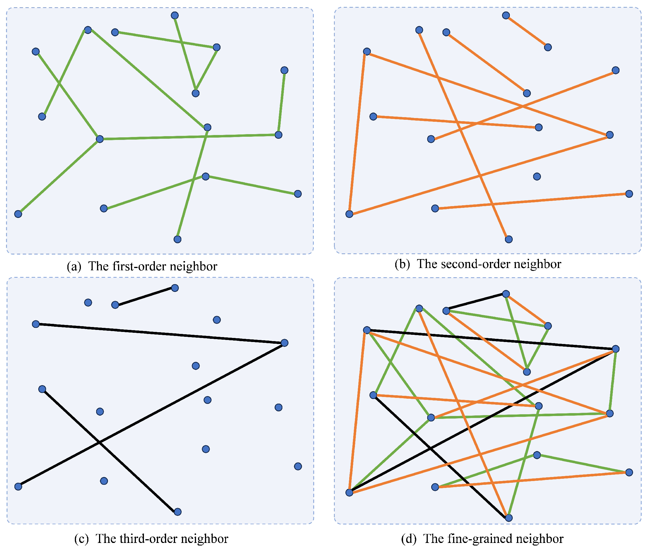
Then, we define P as the Markov transition probability matrix based on S, and , where reveals the probability of data point randomly walking to data point , and D is a diagonal matrix with . Research has found that there is a close connection between the Markov transition probability matrix and the self-expression [12]. Markov random walks tend to occur primarily within clusters, rarely crossing over to other clusters, which indicates that the Markov transition matrix can also capture the neighbor information of the data. This property has an essential advantage in measuring the relationships of the data. In fact, the Markov transition probability matrix mentioned above preserves the one-step neighbor relationships of the data. However, there are not only one-step neighbor relationships between samples but also higher-order neighbor relationships [13]. These relationships reveal the latent neighbor relationships of the samples, which are essential to fully exploit the comprehensive structures of the data. All types of relationships are visualized in Figure 1.
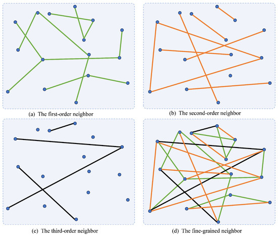
Figure 1.
Visual illustration of neighbor relationships of different orders.
3. Related Work
In this section, we briefly review several classic subspace clustering methods.
3.1. Low-Rank Representation
LRR seeks a low-rank representation of the data with the following minimization problem [8]:
where is the sum of the column-wise norms of a matrix, is the nuclear norm, and is a balancing parameter.
3.2. Sparse Subspace Clustering
SSC assumes a sparse representation of the data, which leads to the following [9]:
where is a balancing parameter. converts the diagonal elements of the input matrix into a column vector; prevents the model from obtaining a trivial solution.
3.3. Robust and Efficient Subspace Segmentation via Least Squares Regression
Robust and Efficient Subspace Segmentation via Least Squares Regression (LSR) utilizes the least squares method to process the expression matrix and introduces the Frobenius norm to seek the low-rank representation of the data [14]. The basic model of LSR involves
Many studies have expanded on these methods, such as block diagonal representation, nonlinear extension, and so on [15,16,17,18].
4. Proposed Method
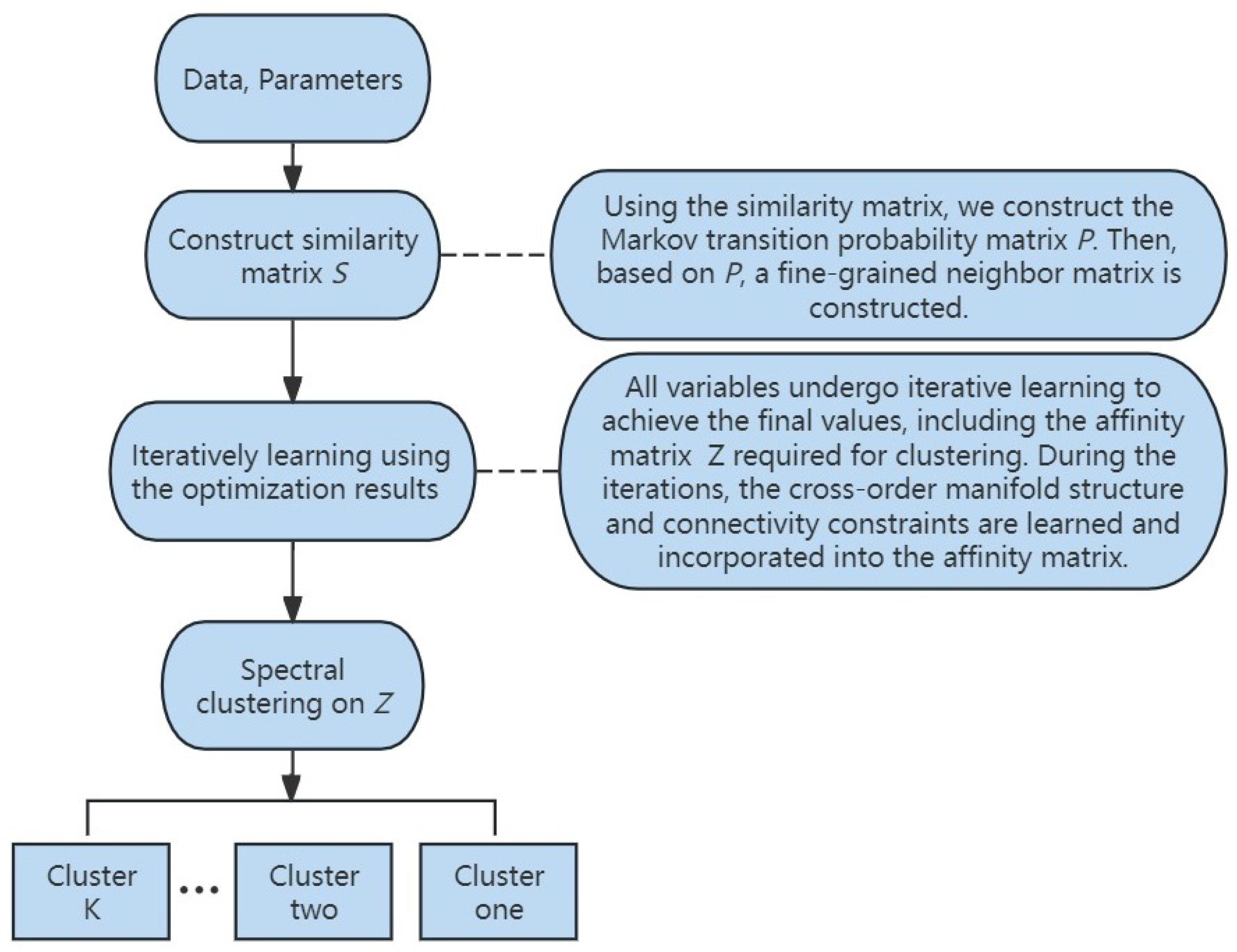
In Figure 2, we illustrate the flowchart of the proposed method. Firstly, the data matrix and parameters are provided as inputs. Subsequently, the similarity matrix is derived from the data, which is used to compute the Markov transition probability matrix and the fine-grained neighborhood matrix. After this, leveraging the optimization results from Section 5, all variables are iteratively solved. Finally, spectral clustering as described in Section 5 is performed on affinity matrix Z, resulting in the final clustering outcome.
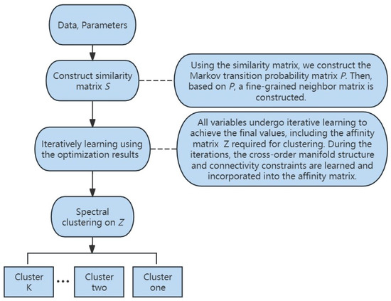
Figure 2.
The flowchart of Markov-Embedded Affinity Learning with Connectivity Constraints for Subspace Clustering (MKSC).
As described in Section 2, the representation matrix obtained from the self-expressive property preserves the similarity information of the data. Meanwhile, the Markov transition probability matrix retains the neighbor information. Generally, samples that are neighbors to each other tend to have higher similarity. Inspired by this, in order to retain the discriminative similarity and neighbor information of the data, we embed the Markov transition probability matrix into the self-expression framework and obtain the following model:
where is the balance parameter and P is the Markov transition probability matrix. In Equation (6), P reveals the one-step random walk probability of the samples, which directly fuses such information with subspace clustering. However, it is insufficient to only adopt the first-order neighbor information. Besides the first-order neighbor information, high-order neighbor information is also important. This type of relationship can preserve more potential structures between the samples and improve the clustering capability of the algorithm. The high-order neighbor relationships of samples can be measured by the probability of a multi-step random walk. In order to fully mine the high-order neighbor information, we define as the high-order Markov transition probability matrix, which reveals the probability of establishing a neighbor relationship between any two samples through a random walk and is defined as
Using to preserve the -order neighbor information of the data, we may recover the latent structure of the data in the representation matrix. To fully utilize the diverse-order neighbor information of the samples, we propose a fine-grained neighbor matrix:
where N is the highest order of the sample neighbor information. Here, the matrix transpose ensures the symmetry of the neighbor relation, which is natural and necessary. Since preserves the high-order neighbor relationships and complementary information, we adopt to further extend our model as
In Equation (9), we construct a fine-grained neighbor matrix through the Markov transition probability matrix. At the same time, this fine-grained neighbor matrix is embedded into the self-expression framework of subspace clustering.
However, nonlinear structures commonly exist in real-world data and are crucial in revealing the underlying true structural information. In order to better deal with the nonlinear relationships, manifold learning is often integrated into the learning model to capture the latent structures of the data on a manifold. Differing from the traditional manifold learning used in [16], we propose to use the cross-order neighbor graph for manifold learning, which enables our model to capture the comprehensive latent structures of the data. Thus, our model is developed as
where , is the graph Laplacian matrix of the fine-grained neighbor matrix , , is a vector with all elements being 1, and converts the input vector into a diagonal matrix. The affinity matrix Z in Equation (10) essentially reveals the correlation of the data, which is expected to have non-negativity and symmetry properties in our model. Thus, the matrix Z can be treated as a connected graph and is significant if it contains k connected components that correspond to the k clusters of the data. According to the Ky Fan theorem, ideally, the number of zero eigenvalues of the Laplacian matrix of Z is equal to the number of connected components in Z. In order to better ensure this property, we further impose a connectivity constraint in our model. We define the graph Laplacian matrix of Z as ; then, the connectivity constraint can be expressed as [15], where is the i-th smallest eigenvalue of the input matrix. Since the connectivity constraint is more efficient in preserving the data structure information and helps as a penalty, we replace the Frobenius norm with the connectivity constraint and further develop our model as
where . In Equation (11), , as a connectivity constraint, can effectively partition the connected components on the graph and connect the samples within the clusters. This characteristic of the connectivity constraint can improve the algorithm’s ability to handle the group structure of the data, thereby enhancing the clustering performance.
It is noted that there are excessive restrictions on the affinity matrix Z in the model. These restrictions may limit the expression of Z. Thus, we introduce an intermediate variable B to alleviate this problem in a way similar to [15]:
where , and, when , by minimizing Equation (12), we can make . Moreover, introducing ensures that the subproblems related to Z and B are strongly convex, which is more convenient for optimization. Equation (12) is named Markov-Embedded Affinity Learning with Connectivity Constraints for Subspace Clustering (MKSC). MKSC has four balancing parameters: . In Equation (12), controls the speed at which matrix Z and B become similar. The larger the value of , the faster Z and B become similar, and vice versa. Similar to , controls the speed of approximation between and Z. The larger the value of , the faster and Z approximate each other, and vice versa. For , the larger is, the stronger the connectivity constraint on the affinity matrix Z. controls the manifold, which can affect the model’s ability to handle nonlinear data.
5. Optimization
In this section, we give the complete optimization process of Equation (12). Firstly, we reformulate Equation (12) in the following manner [15]:
where I is an identity matrix.
5.1. Optimization of Variable W
Fixing the variables Z and B, we can obtain the subproblem with respect to W:
According to [19], the closed-form solution for W is
where H is the matrix composed of the eigenvectors corresponding to the k smallest eigenvalues of .
5.2. Optimization of Variable B
Fixing the variables Z and W, we can obtain the subproblem with respect to B:
By calculation, Equation (16) is equivalent to
For convenience in calculation, we define and let , and then we substitute A into Equation (17):
The closed-form solution for Equation (18) is [15]
where , is the non-negative projection of the matrix, and .
5.3. Optimization of Variable Z
Fixing the variables W and B, we can obtain the subproblem with respect to Z:
Obviously, Equation (20) is convex, and, by taking the derivative of Equation (20), we obtain
We repeat the above steps until convergence. For clarity, we summarize the above optimization process in Algorithm 1.
| Algorithm 1 Markov-Embedded Affinity Learning with Connectivity Constraints for Subspace Clustering |
After we solve Equation (13), we use Z to construct A in a standard post-processing manner, as in [20]. Following [20], we construct A with the following steps. (1) We compute the skinny SVD of Z as and define to be the weighted column space of Z. (2) We obtain the normalized matrix by normalizing each row of . (3) The affinity matrix A is constructed as , where the parameter controls the sharpness of the affinity matrix between samples. (4) Finally, we perform Normalized Cut (NCut) [21] on A in a manner similar to [20,22].
5.4. Complexity Analysis
In this subsection, we analyze the computational complexity as follows. In Equation (15), the size of H is . Therefore, updating W requires complexity of . For B, the computational complexity is . In Equation (21), the complexity of is . Due to the inversion operation, the complexity of is . Simultaneously, the complexity of is . Therefore, for Z, the computational complexity is . Overall, the total complexity can be written as in each iteration. The dominant complexity arises from the inversion of the matrix and the multiplication of the matrix, both of which have complexity of . For multiplication, we can solve this through parallel computation. For inversion, we note the special structure. This part is composed of the sum of the diagonal matrix and the low-rank matrix. Ref. [23] provides a potential method for acceleration.
6. Experiments
To verify the effectiveness of MKSC, extensive experiments are conducted in this section.
6.1. Research Methodology
In this subsection, we introduce the details of the research methodology. We seek to verify the effectiveness of the proposed method by raising the following questions.
- Can the proposed method achieve excellent clustering performance in various real application scenarios?
- Can high-order neighbor information improve the clustering performance of the proposed method?
- Does the high-order neighbor manifold structure enable the method to effectively handle nonlinear data?
- Can the connectivity constraint guarantee the group structure of the affinity matrix?
- Can the learned affinity matrix preserve the key information of the original data?
To answer these questions, we design a comprehensive series of experiments. First, we validate the clustering performance of the algorithm, including its accuracy, speed, sensitivity to parameters, and the ability to handle nonlinear data. In particular, the proposed method is compared with several state-of-the-art baseline methods regarding their clustering performance on three types of real application data sets using five clustering evaluation metrics. The speed of the proposed method is validated using a convergence analysis and the clustering time cost in Section 6.3.3 and Section 6.3.5. An algorithm that is insensitive to the parameters can be applied to more potential scenarios. Therefore, we conduct parameter sensitivity experiments in Section 6.3.7. In Section 6.3.2, the proposed method is compared with the baseline methods on a nonlinear data set. Second, we verify the impact of the high-order neighborhood information, the connectivity constraints, and the novel manifold term on the clustering performance of the proposed algorithm in Section 6.3.6. Third, we validate the ability of the learned affinity matrix of the proposed algorithm to capture key information. Generally, the number of block diagonals in the affinity matrix is equal to the number of clusters in the data. Therefore, we visualize the learned representation matrix in Section 6.3.4. Meanwhile, to validate the ability of the affinity matrix to preserve neighbor information, we demonstrate the changes in the distribution of the original data and clustered data in Section 6.3.4. In fact, by identifying key features, the data can be effectively partitioned into different clusters. In Section 6.3.8, by utilizing the self-expressive property, we visually compare the reconstructed images of X and in order to demonstrate the ability of the affinity matrix to preserve key features.
The details of the five evaluation metrics are as follows [24,25,26].
Accuracy (ACC) is defined as
where and represent the predicted and true labels of the data point , respectively. maps each cluster label to the equivalent label from the data set by permutation such that (22) can be maximized, and is the delta function, which returns 1 when or 0 otherwise.
Normalized mutual information (NMI) is defined as
where and denote the sizes of the -th cluster and -th class, respectively. denotes the number of data points that are present in the intersection between them, and M is the number of clusters.
Purity (PUR) is defined as
where is the number of data points in the -th cluster that belong to the -th class. PUR measures the extent to which each cluster contains data points from primarily one class. More details about these measures can be found in [27].
The F-score (FS) is defined as
where and . Here, (True Positive) indicates the number of cases where two samples belonging to the same class are grouped into the same cluster. (False Positive) occurs when two samples belonging to different classes are grouped into the same cluster. (False Negative) occurs when two samples belonging to the same class are grouped into different clusters. and often exhibit a trade-off relationship, where improving one metric may occur at the cost of reducing the other. FS is a comprehensive balance between and . In (25), is the balance parameter. When , and are equally important. Without loss of generality, we set to 1.
The Adjusted Rand Index (ARI) is defined as
where quantifies the ratio of correct decisions. , where indicates the total number of pairs that can be formed from the sample. is the expectation operator, and the ARI is an adjusted version of that takes values in . The larger the ARI, the more consistent the clustering results are with the true clustering structure.
6.2. Experimental Setup
In this subsection, we introduce the details of the experimental setup. Comparison experiments are conducted in Matlab 2018a on a machine with an Intel (R) Core (TM) i7-8700 CPU @ 3.20G Hz and 32.0 G memory. The time cost study is executed in Matlab 2018a on a machine with an 11th-Gen Intel Core i7-11700T CPU @ 1.40 GHz and 16 G memory.
In certain scenarios (e.g., classification), the label information of the data is crucial. However, it is generally expensive to manually label unlabeled data. Clustering can directly and effectively produce fairly accurate labeling results. This can greatly enhance the work efficiency and guarantee the operational performance. To verify the universality of the proposed method’s labeling capability, we enumerate three real application scenarios to conduct the experiments, including faces, handwritten digits and letters, and actions. Figure 3 shows some examples of these eight data sets.
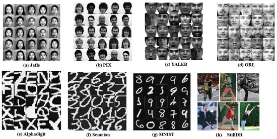
Figure 3.
Examples of images selected from three different real application data sets.
Firstly, on the face real application data sets, we perform clustering based on the facial features of different individuals, with all images of the same individual grouped into one cluster. The details of these data sets are as follows. The Jaffe data set contains 213 images, collected from 10 Japanese female students making 7 facial expressions, and each image’s size is 26 × 26 pixels. The PIX data set comprises 100 images of 10 objects, with each image sized at 100 × 100 pixels. The YALEB data set contains 165 grayscale face images of 15 individuals; all images are 32 × 32 pixels. The ORL data set includes face images of 40 different individuals, with each individual represented by 10 images. Each image measures 32 × 32 pixels. Secondly, on the real application datasets of handwritten digits and letters, we obtain the final clusters based on the categories of handwritten digits 0–9 and letters A–Z. This allows all images of the same digit or letter to be grouped into the same cluster. The details of these data sets are as follows. The Binary Alphadigits (Alphadigit) data set contains 36 categories of digits 0–9 and letters A–Z, each category has 39 images, and each image is 20 × 16 pixels. The Semeion Handwritten Digit (Semeion) data set contains 1593 handwritten digit images from 80 people, encompassing 10 categories. Each image is 16 × 16 pixels and features 256 gray levels. The Modified National Institute of Standards and Technology (MNIST) data set comprises 7000 images of digits 0–9. For this experiment, we randomly select 400 images; each image is 28 × 28 pixels. Among these images, 50% are collected from high school students and 50% from the Census Bureau. Finally, on the Still Images (StillDB) action real application data set [28], we group the images into different clusters based on different actions. The StillDB data set comprises 467 images, encompassing six distinct actions: running, walking, catching, throwing, crouching, and kicking.
We compare the proposed method with ten baseline methods, namely Non-Negative Sparse Hyper-Laplacian Regularized LRR (NSLLRR) [29], SSC [9], Subspace Clustering Using Log-Determinant Rank Approximation (SCLA) [20], Scaled Simplex Representation for Subspace Clustering (SSRSC) [30], S-TLRR [31], R-TLRR [31], Tensor Low-Rank Sparse Representation for Tensor Subspace Learning (TLRSR) [32], Enhanced Tensor Low-Rank Representation for Clustering and Denoising (ETLRR) [33], Efficient Deep Embedded Subspace Clustering (EDESC) [34], and Pseudo-Supervised Deep Subspace Clustering (PSSC) [35]. Among them, the first four are traditional subspace clustering methods, the last two are deep subspace clustering methods, and the remaining four are tensor-based subspace clustering methods. For all methods, the range of the balance parameter is , the binary kernel is used in this experiment, and 5 neighbors are retained to construct the similarity matrix. The order of the fine-grained neighbor matrix is set to 3. For EDESC, we set the parameters according to [34], with set within the range and d and set within the range . For the parameters of PSSC, they are set according to [35]. A three-layer convolutional network with a depth set to and a kernel size set to is employed. For each method, the experiment considers all combinations of parameters.
Brief descriptions of each method are provided in the following. (1) NSLLRR extends LRR on manifolds. We construct the similarity matrix using a binary weighting strategy and retain 5 neighbors on the graph. (2) SSC is a classic method that uses the L-1 norm as a regularization term to achieve sparse representation on the coefficient matrix. (3) SCLA is another type of extension of LRR that approximates the rank with a non-convex LDRA rather than the NN. (4) SSRSC recovers physically meaningful representations. For its parameters, we follow the original paper. (5) S-TLRR and R-TLRR are different forms of TLRR. TLRR is an approach that can exactly recover the clean data of an intrinsic low-rank structure and accurately cluster them as well. S-TLRR and R-TLRR handle slightly and severely corrupted data, respectively. (6) TLRSR can directly perform subspace learning on three-dimensional tensors. (7) ETLRR decomposes the original data tensor into three parts: a low-rank structure tensor, a sparse noise tensor, and clustering. (8) EDESC learns a set of subspace bases from the latent features extracted by a deep auto-encoder, where the bases and network parameters are iteratively refined. (9) PSSC integrates the deep SC and pseudo-supervision to obtain the similarity matrix. By utilizing pseudo-supervision, it enables the model to have better feature extraction and similarity learning capabilities.
6.3. Results
We compare our method with the ten baseline methods on three different real application data sets and demonstrate the effectiveness of the method through a series of visualization methods in this subsection.
6.3.1. Clustering Results of Real Application Data Sets
In this subsection, we assess the clustering performance of the baseline methods and MKSC. For each individual method, we tune its parameters as described in Section 6.2.
In Table 1, Table 2, Table 3, Table 4 and Table 5, we present the clustering performance of all methods on the face real application data sets. It can be observed that on the face real application data sets, the proposed method is the best clustering method, achieving the best clustering performance in 16 out of 20 cases. Several baseline methods also perform well in certain scenarios. For example, PSSC achieves top-two performance in the FS metric. However, the clustering performance of PSSC still lags behind that of the proposed method.

Table 1.
Clustering ACC on face real application data sets.
Table 2.
Clustering NMI on face real application data sets.
Table 3.
Clustering PUR on face real application data sets.
Table 4.
Clustering FS on face real application data sets.
Table 5.
Clustering ARI on face real application data sets.
In Table 6, Table 7, Table 8, Table 9 and Table 10, we present the clustering performance of all methods on the handwritten digit and letter real application data sets. In all cases, the proposed method achieves the best performance. Among the baseline methods, the most competitive methods are SCLA and SSRSC. However, their clustering performance still lags significantly behind that of the proposed method. For example, in terms of the NMI evaluation metric, the MKSC algorithm outperforms SCLA by 5.96%, 11.29%, and 12.17%, respectively, on three different real application data sets.
Table 6.
Clustering ACC on handwritten digit and letter real application data sets.
Table 7.
Clustering NMI on handwritten digit and letter real application data sets.
Table 8.
Clustering PUR on handwritten digit and letter real application data sets.
Table 9.
Clustering FS on handwritten digit and letter real application data sets.
Table 10.
Clustering ARI on handwritten digit and letter real application data sets.
In Table 11, we present the clustering performance of all methods on the StillDB data set. Compared to the baseline methods, the proposed method achieves the overall best performance across five metrics. Although the proposed algorithm takes second place in the PUR metric, it only lags behind the first-place SCLA by approximately 1%.
Table 11.
Clustering results on action real application data sets.
Specifically, we analyze the evidence of the superiority of the proposed method as follows. The proposed method is compared with three types of algorithms. First, compared with traditional subspace clustering, the proposed method performs better, mainly due to the utilization of the fine-grained neighborhood matrix. The application of this matrix significantly improves the ability of the algorithm to preserve the latent information and handle nonlinear data. At the same time, the introduction of connectivity constraints also enhances the group structure of the affinity matrix. Second, when compared with tensor subspace clustering, the proposed method does not involve flattening or folding operations on the matrix, thus reducing the potential for information loss. Finally, deep subspace clustering algorithms often require a large amount of samples for learning. In this paper, the size of the data sets is relatively small, potentially resulting in the model not being fully utilized. Specifically, the EDESC algorithm, which deviates from the self-expressive framework, is more suitable for large data sets.
6.3.2. Clustering Results on Toy Data Set
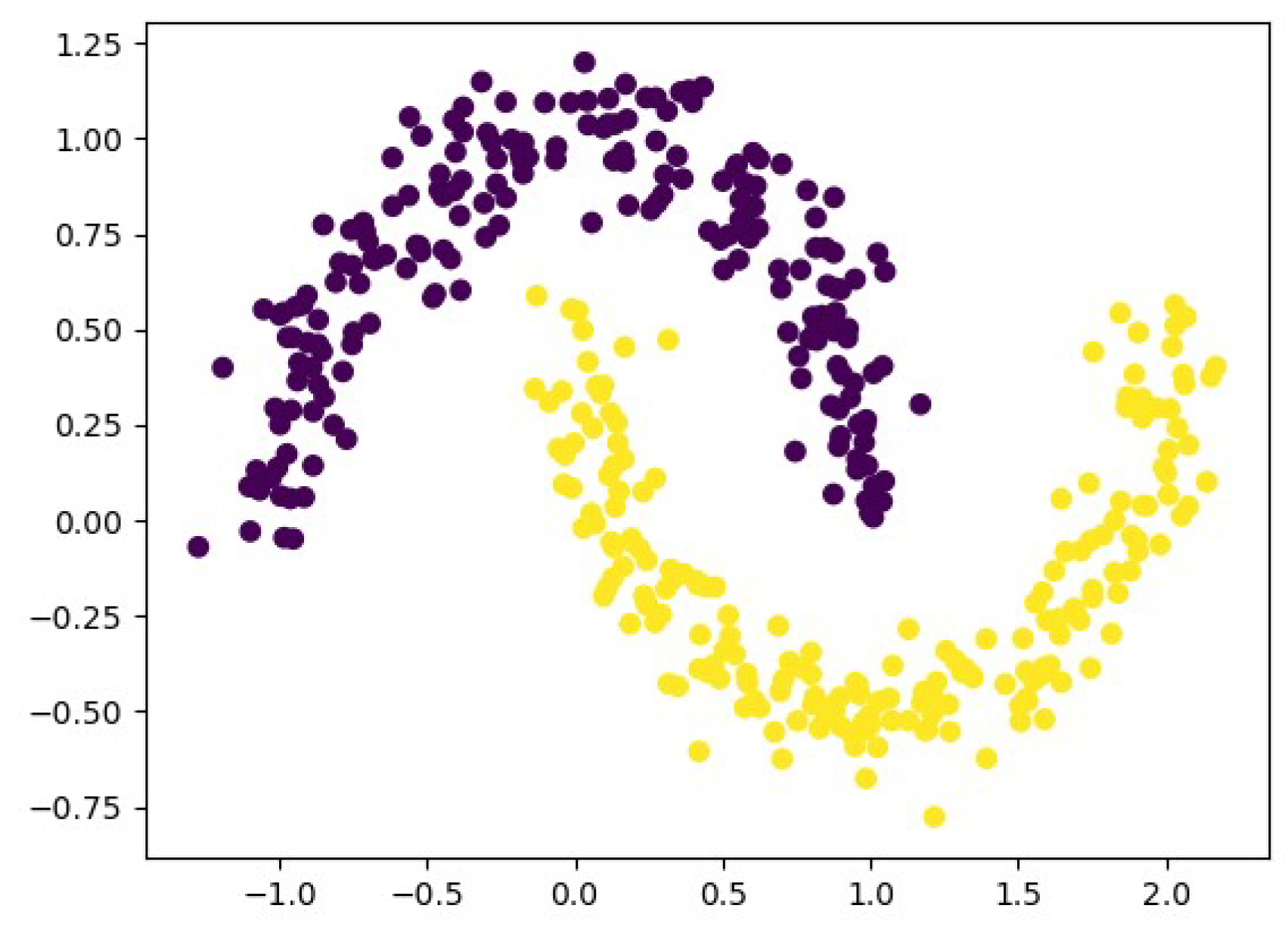
In this subsection, we use the nonlinear moon data set to validate the ability of the proposed algorithm to handle nonlinear data. The moon data set can intuitively demonstrate the nonlinear structures among data. Specifically, the moon data set consists of two parts, represented by purple and yellow. Although some samples of the purple and yellow parts are close to each other, they actually belong to different clusters. However, the two ends of the purple or yellow parts, which are far apart, still belong to the same cluster. The generation of the moon is as follows. First, a data matrix of size is randomly generated, where N represents the number of samples, which we set to 400. Subsequently, data labels corresponding to the N samples are generated, with a total of two classes. Finally, noise is added to the data, and the noise level is set to 0.1. We provide an example of the moon data set in Figure 4.

Figure 4.
Examples of moon data set.
In Table 12, we demonstrate the clustering results of the baseline method and the proposed method on the moon data set. It can be observed that the proposed algorithm exhibits significant advantages on the moon data set. This indicates that the proposed algorithm can effectively handle complex nonlinear data relationships, thereby improving the clustering performance.
Table 12.
Clustering results on moon data set.
6.3.3. Time Cost
In this test, we conduct experiments to verify the efficiency of the proposed method. Because the clustering accuracy is the key focus, we only compare our method with the most competitive baseline methods, i.e., SCLA and NSLLRR. In particular, the experiments are conducted in Matlab 2018a on a machine with an 11th-Gen Intel Core i7-11700T CPU@1.40 GHz and 16 G memory (Intel, Santa Clara, CA, USA), for which the results are reported in Figure 5.
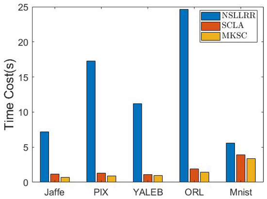
Figure 5.
Time costs of different methods on various data sets.
From the results, it can be seen that MKSC is much faster than NSLLRR and comparable to SCLA. Considering that MKSC has superior clustering performance, the time cost of MKSC is fairly acceptable.
6.3.4. Learned Representation
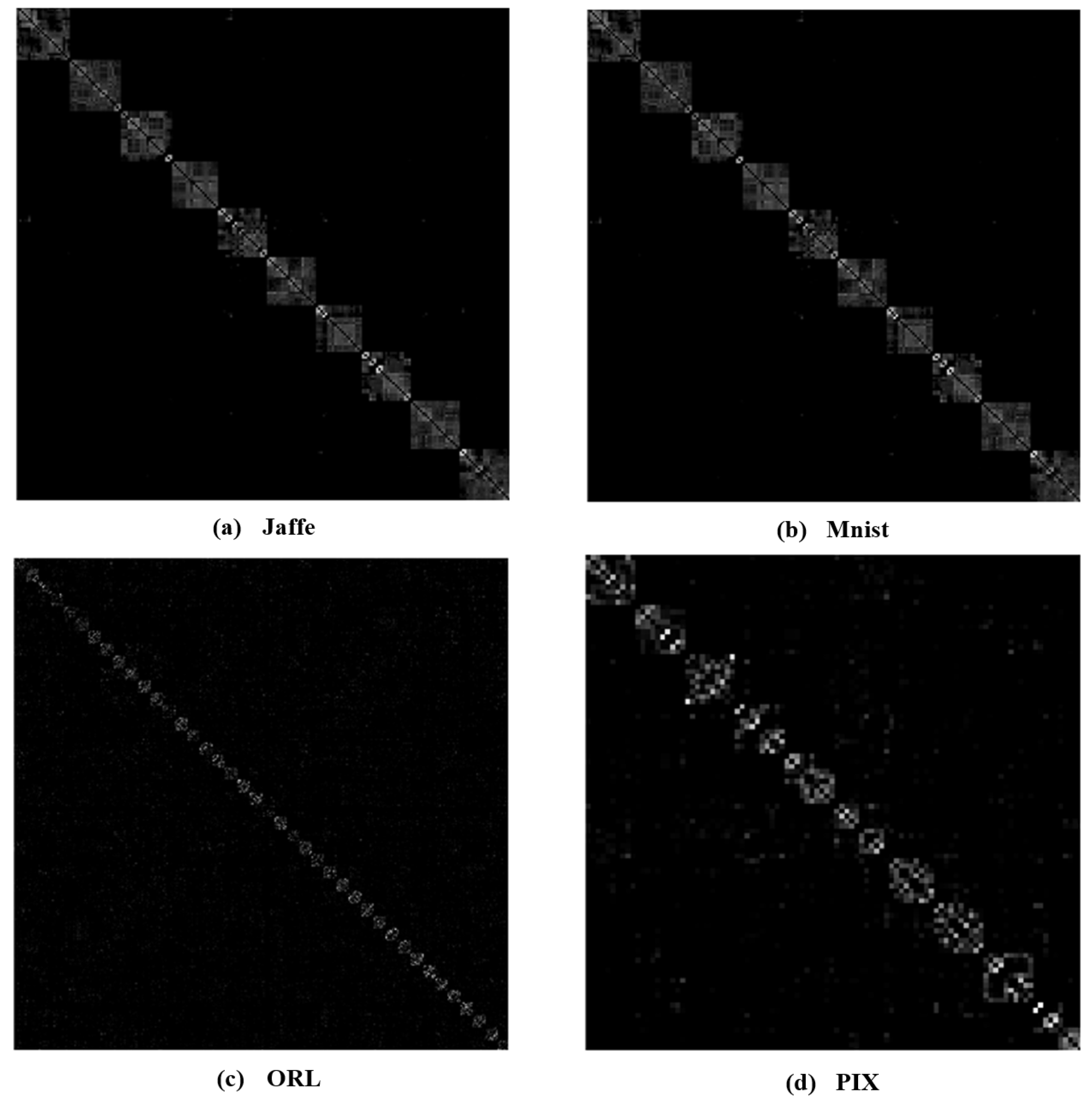
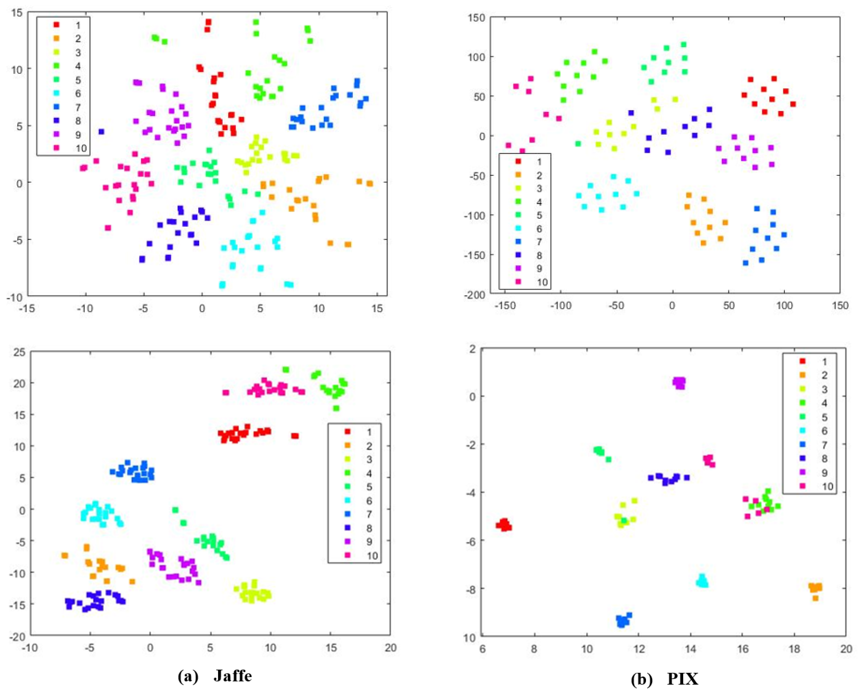
To better investigate the learning capabilities of MKSC, we visually show the group structure of the representation matrix Z learned by MKSC. In particular, we show the results on the Jaffe, MNIST, ORL, and PIX data sets in Figure 6. It can be seen that the representation matrices have clear block diagonal structures, which correspond to the clusters of the data sets. Moreover, we visualize the data points of Jaffe and PIX in Figure 7, with t-distributed stochastic neighbor embedding (t-SNE) [36]. In Figure 7, the first and second rows are the original data and the t-SNE visualization of the representation matrix Z, respectively. It is seen that the samples are overlapped with the original features and are well separated with the similarity graph. These observations visually confirm the effectiveness of MKSC in recovering the group structures of the data.
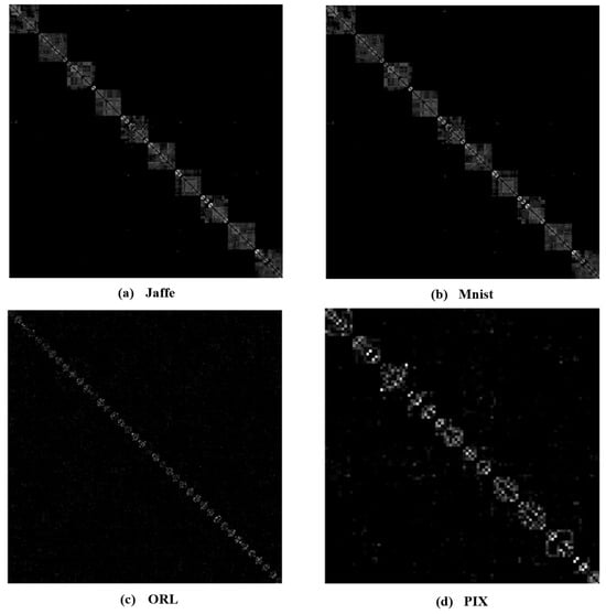
Figure 6.
Examples of the learned representation matrix Z.
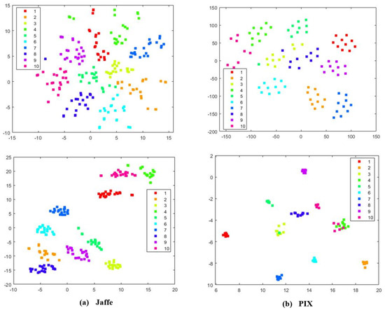
Figure 7.
The t-SNE visualization of the Jaffe and PIX data sets, respectively. The first and second rows correspond to the t-SNE visualization of the original data and the reconstructed representation on Jaffe and PIX, respectively.
6.3.5. Convergence Analysis
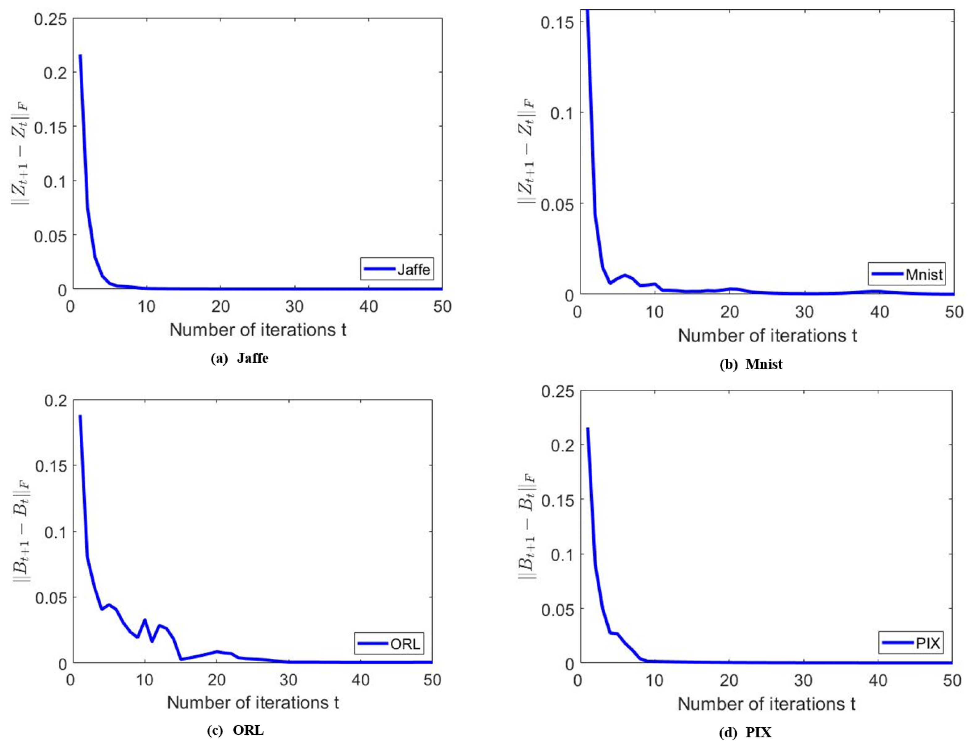
To empirically verify the convergence of the proposed algorithm, we show some experimental results for a clearer illustration. For the sake of generality, we show the results on the Jaffe, MNIST, ORL, and PIX data sets. To show the convergence properties of and , we plot the values of and for the first 50 iterations in Figure 8. We can observe that both and converge to zero within about 50 iterations, which confirms the efficiency and convergence of the MKSC algorithm.
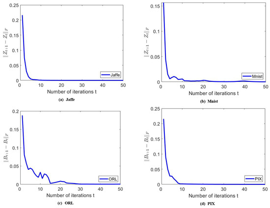
Figure 8.
Examples to show the convergence of , on different data sets.
6.3.6. Ablation Study
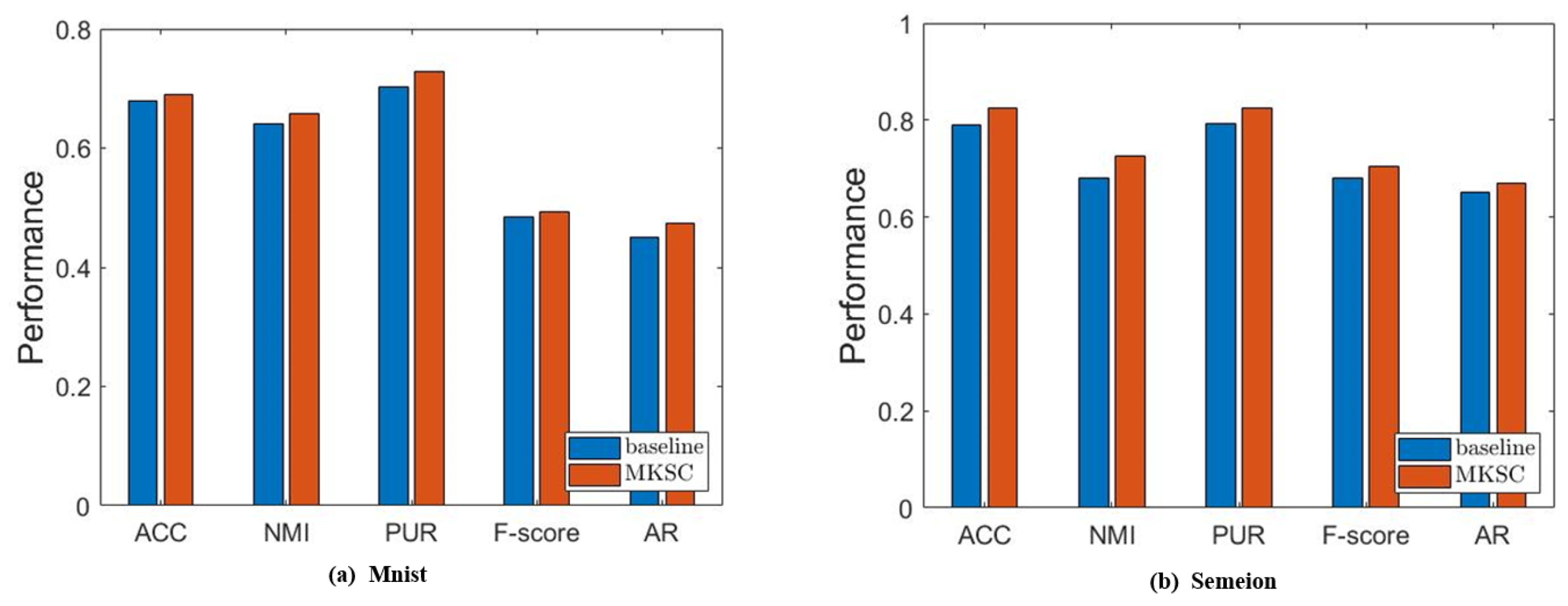
In this subsection, we validate the effectiveness of the embedded Markov transition probability information. First, we show some empirical results to confirm the effectiveness of the Markov transition probability information and the high-order neighbor information. Without loss of generality, we conduct ablation experiments on the MNIST and ORL data sets. In particular, we set and treat the model as the baseline, while the other parameters are tuned in the same way as in Section 6.2. Specifically, we tune the other balancing parameters within and report the highest clustering performance in Figure 9.

Figure 9.
Results of comparison between MKSC and comparison method on MNIST and Semeion.
It is observed that MKSC has better performance than the baseline, which confirms the effectiveness of the Markov transition probability information and high-order neighbor information used in the MKSC model. Then, we validate the effect of the connectivity constraints on the group structure. The clustering performance is closely related to the group structure. Generally speaking, excellent clustering performance indicates a clear group structure. Therefore, we conduct an ablation study by setting to verify the impact of the connectivity constraints on the group structure. As shown in Figure 10, the connectivity constraints improve the clustering performance, indicating that the connectivity constraints make the group structure clearer.
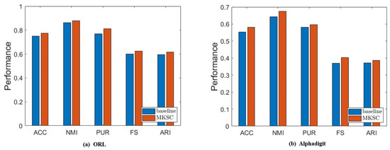
Figure 10.
Results of comparison between MKSC and comparison method on ORL and Alphadigit.
Furthermore, we conduct an ablation study to discuss the complexity of the nonlinear relationships that can be handled by the proposed method. We validate the capability of the manifold term on three data sets, including faces, handwritten digits, and actions. The complexity of the nonlinear relationships in these data sets is different. We set to 0 in order to validate the ability of the proposed cross-order manifold term to handle nonlinear relationships of different complexity levels. Figure 11 demonstrates that on the three types data sets, the proposed manifold term consistently enhances the clustering performance of the algorithm, enabling it to tackle nonlinear relationships of varying complexity effectively.
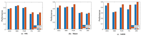
Figure 11.
Results of comparison between MKSC and comparison method on ORL, MNIST, and StillDB.
6.3.7. Parameter Sensitivity
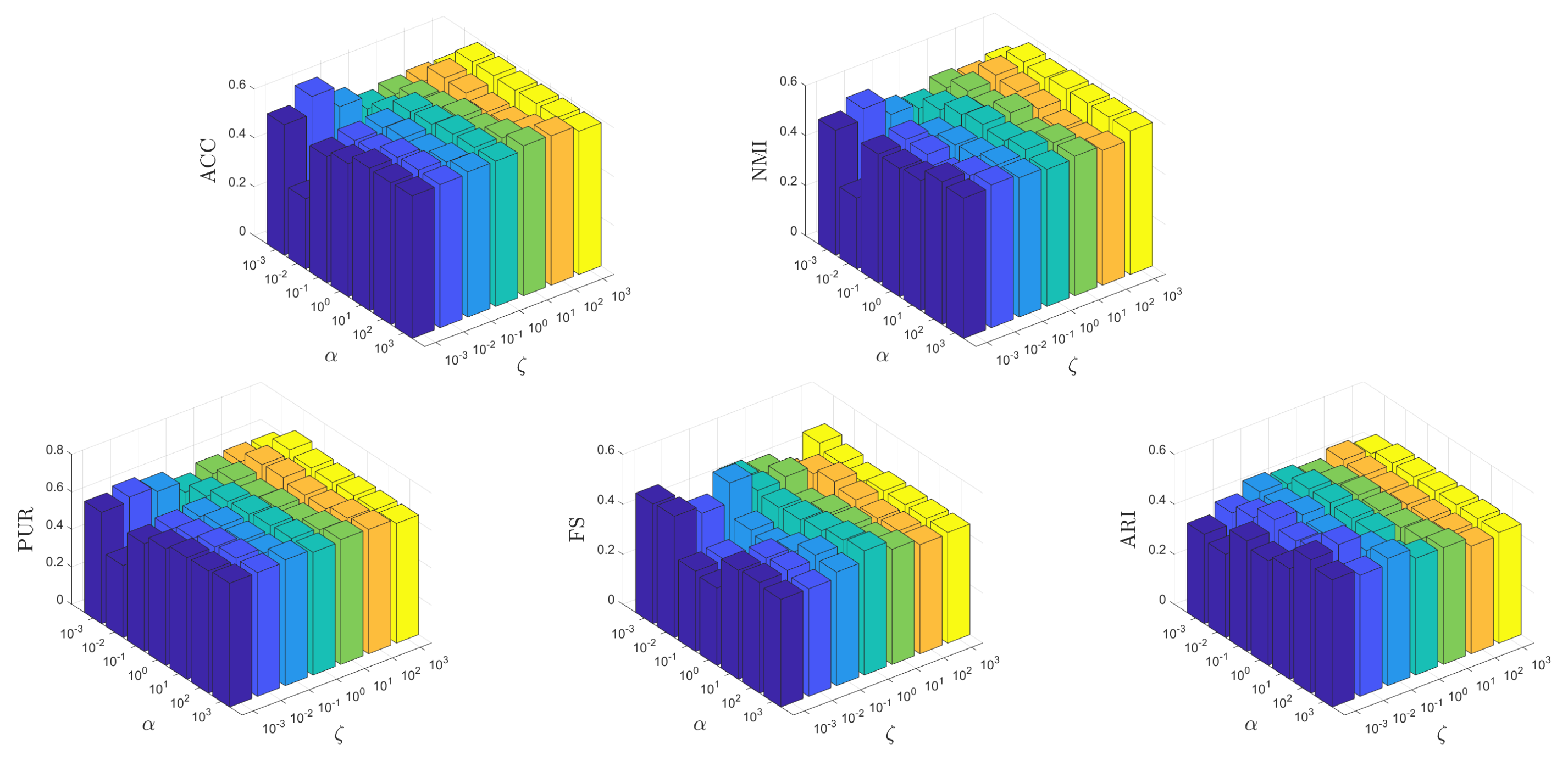
It is crucial for an unsupervised learning method to be insensitive to the parameters to ensure its potential applicability in real-world scenarios. In this test, we conduct experiments to show how the parameters affect the learning performance of MKSC, where, without loss of generality, we show the results on the MNIST data set. Firstly, we show the effects of different combinations of on the MNIST data set. Both and vary within the range of , while and are fixed to their optimal values. Secondly, we investigate the impact of various combinations of on the MNIST data set. Both and are varied within the range of while keeping and constant at their respective optimal values. This analysis aims to assess the performance sensitivity of our approach with respect to these parameters.
From Figure 12 and Figure 13, it can be observed that the MKSC algorithm is quite insensitive to the parameters on the MNIST data set in all metrics. These observations indicate that the MKSC algorithm is insensitive to the parameters, suggesting its potential suitability for unsupervised learning problems.

Figure 12.
Clustering performance of MKSC with combination of on MNIST data set.
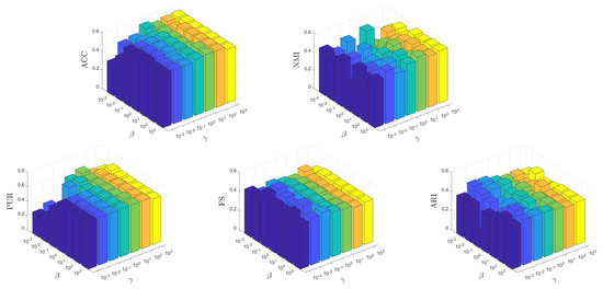
Figure 13.
Clustering performance of MKSC with combination of on MNIST data set.
In particular, we explain the impact of the parameters on the algorithm performance. In Figure 12, the impact of is small. When is set to , MKSC performs well. The impact of is also slight, and the overall performance remains stable. In Figure 13, when beta is set to , the performance overall remains good. Similar to , the variation in has a small impact on the algorithm’s performance.
6.3.8. Data Reconstruction
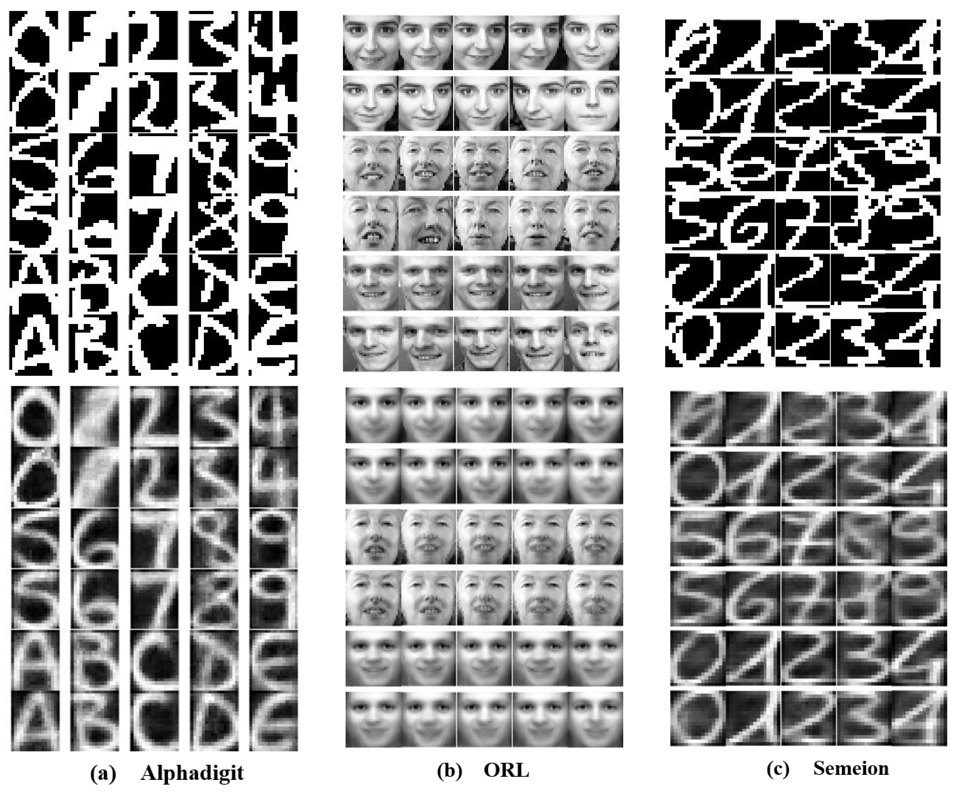
To validate the capability of the affinity matrix in preserving key features, we present a comparison of the reconstructed images from X and in Figure 14. Without loss of generality, we perform experiments on the Alphadigit, ORL, and Semeion data sets. All parameter settings are the same as in Section 6.2. It is seen that the reconstructed images contain the key features of all original samples. For example, in Figure 14, the original Semeion images of digit 4 appear distinct, but, in the reconstructed Semeion images of XZ, the key features of the original images of digit 4 are preserved, and they share very high similarity. Meanwhile, in Figure 14, although the original ORL images of the same person have different facial expressions or orientations, the reconstructed ORL images of XZ still share a high degree of similarity. Therefore, the affinity matrix Z effectively retains the key information from the original data.
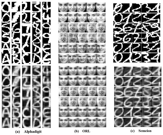
Figure 14.
Comparison of data reconstruction effects. The first and second rows correspond to the effects of the original and reconstructed data, respectively.
6.4. Discussion
It can be observed that the proposed method achieves the best clustering performance on the three real application data sets compared to the baseline methods. While the baseline methods may perform exceptionally well in some cases, they do not consistently do so. In terms of computational speed, the proposed algorithm converges quickly and the time cost of clustering is also highly competitive. In data reconstruction, it can be seen that the proposed method is able to retain the key features of the original data. It is observed that the learned representation matrix has clear block diagonal structures. Simultaneously, as can be seen from the t-SNE visualization, the clustered sample points transition from a dispersed state to a compact formation. The ablation study verifies the effectiveness of embedding Markov transition probability information into the self-expression framework. Simultaneously, the ability of the proposed manifold term to handle nonlinear data is also demonstrated in the ablation study. The impact of connectivity constraints on the group structure is also validated in the ablation study. In the parameter sensitivity study, the proposed method maintains good insensitivity across the five clustering evaluation metrics. Overall, the proposed algorithm exhibits excellent capabilities in terms of clustering performance, key feature capture, and computational speed.
7. Conclusions
In this paper, we propose a novel subspace clustering algorithm named MKSC. In MKSC, the Markov transition probability information is embedded into a self-expression framework, preserving the diverse clustering characteristics. Additionally, a fine-grained neighbor matrix is employed to comprehensively capture the cross-order neighbor relationships and complementary information among samples. To better handle nonlinear data, MKSC leverages the manifold structure of cross-order local neighbor graphs. Furthermore, connectivity constraints are imposed on the affinity matrix to enhance the grouping structure. The experiments show that the proposed method is better than the current popular methods on real application cases.
It should be noted that noise and outliers are widely present. However, MKSC mainly considers clean data. Therefore, when dealing with data that are heavily influenced by noise, it may become less robust. Moreover, with the increasing diversity of information media, the processing of multi-view data is also a key issue. However, the MKSC algorithm only focuses on single-view data, necessitating the conversion of multi-view data into a single-view format for its application. In the future, we will further refine the algorithm to effectively handle multi-view data and achieve greater robustness.
Author Contributions
Conceptualization, methodology, software and validation, W.S. and X.Z.; formal analysis, investigation, data curation, writing—original draft preparation and visualization, W.S.; resources, writing—review and editing, supervision, project administration and funding acquisition, X.Z. All authors have read and agreed to the published version of the manuscript.
Funding
This research received no external funding.
Institutional Review Board Statement
Not applicable.
Informed Consent Statement
Not applicable.
Data Availability Statement
Data is contained within the article.
Conflicts of Interest
The authors declare no conflict of interest.
References
- Peng, C.; Chen, Y.; Kang, Z.; Chen, C.; Cheng, Q. Robust principal component analysis: A factorization-based approach with linear complexity. Inf. Sci. 2020, 513, 581–599. [Google Scholar] [CrossRef]
- Zhang, X.; Cheng, L.; Li, B.; Hu, H.M. Too Far to See? Not Really!—Pedestrian Detection with Scale-Aware Localization Policy. IEEE Trans. Image Process. 2018, 27, 3703–3715. [Google Scholar] [CrossRef] [PubMed]
- Peng, C.; Cheng, Q. Discriminative Ridge Machine: A Classifier for High-Dimensional Data or Imbalanced Data. IEEE Trans. Neural Netw. Learn. Syst. 2021, 32, 2595–2609. [Google Scholar] [CrossRef] [PubMed]
- Huang, B.; Ge, L.; Chen, G.; Radenkovic, M.; Wang, X.; Duan, J.; Pan, Z. Nonlocal graph theory based transductive learning for hyperspectral image classification. Pattern Recognit. 2021, 116, 107967. [Google Scholar] [CrossRef]
- Peng, C.; Liu, Y.; Kang, K.; Chen, Y.; Wu, X.; Cheng, A.; Kang, Z.; Chen, C.; Cheng, Q. Hyperspectral Image Denoising Using Nonconvex Local Low-Rank and Sparse Separation With Spatial-Spectral Total Variation Regularization. IEEE Trans. Geosci. Remote. Sens. 2022, 60, 1–17. [Google Scholar] [CrossRef]
- Peng, C.; Zhang, J.; Chen, Y.; Xing, X.; Chen, C.; Kang, Z.; Guo, L.; Cheng, Q. Preserving bilateral view structural information for subspace clustering. Knowl. Based Syst. 2022, 258, 109915. [Google Scholar] [CrossRef]
- Du, Y.; Lu, G.F.; Ji, G.; Liu, J. Robust subspace clustering via multi-affinity matrices fusion. Knowl. Based Syst. 2023, 278, 110874. [Google Scholar] [CrossRef]
- Liu, G.; Lin, Z.; Yan, S.; Sun, J.; Yu, Y.; Ma, Y. Robust Recovery of Subspace Structures by Low-Rank Representation. IEEE Trans. Pattern Anal. Mach. Intell. 2013, 35, 171–184. [Google Scholar] [CrossRef] [PubMed]
- Elhamifar, E.; Vidal, R. Sparse Subspace Clustering: Algorithm, Theory, and Applications. IEEE Trans. Pattern Anal. Mach. Intell. 2013, 35, 2765–2781. [Google Scholar] [CrossRef]
- Wang, J.; Shi, D.; Cheng, D.; Zhang, Y.; Gao, J. LRSR: Low-Rank-Sparse representation for subspace clustering. Neurocomputing 2016, 214, 1026–1037. [Google Scholar] [CrossRef]
- Xia, R.; Pan, Y.; Du, L.; Yin, J. Robust Multi-View Spectral Clustering via Low-Rank and Sparse Decomposition. In Proceedings of the AAAI Conference on Artificial Intelligence, Québec City, QC, Canada, 27–31 July 2014; Volume 28. [Google Scholar] [CrossRef]
- Wu, J.; Lin, Z.; Zha, H. Essential Tensor Learning for Multi-View Spectral Clustering. IEEE Trans. Image Process. 2019, 28, 5910–5922. [Google Scholar] [CrossRef] [PubMed]
- Tang, J.; Qu, M.; Wang, M.; Zhang, M.; Yan, J.; Mei, Q. LINE: Large-scale Information Network Embedding. In Proceedings of the 24th International Conference on World Wide Web, Florence, Italy, 18–22 May 2015. [Google Scholar]
- Lu, C.Y.; Min, H.; Zhao, Z.Q.; Zhu, L.; Huang, D.S.; Yan, S. Robust and Efficient Subspace Segmentation via Least Squares Regression. In Proceedings of the Computer Vision—ECCV 2012, Florence, Italy, 7–13 October 2012; Fitzgibbon, A., Lazebnik, S., Perona, P., Sato, Y., Schmid, C., Eds.; Springer: Berlin/Heidelberg, Germany, 2012; pp. 347–360. [Google Scholar]
- Lu, C.; Feng, J.; Lin, Z.; Mei, T.; Yan, S. Subspace Clustering by Block Diagonal Representation. IEEE Trans. Pattern Anal. Mach. Intell. 2019, 41, 487–501. [Google Scholar] [CrossRef] [PubMed]
- Liu, J.; Chen, Y.; Zhang, J.; Xu, Z. Enhancing Low-Rank Subspace Clustering by Manifold Regularization. IEEE Trans. Image Process. 2014, 23, 4022–4030. [Google Scholar] [CrossRef] [PubMed]
- Xiao, S.; Tan, M.; Xu, D.; Dong, Z.Y. Robust Kernel Low-Rank Representation. IEEE Trans. Neural Netw. Learn. Syst. 2016, 27, 2268–2281. [Google Scholar] [CrossRef] [PubMed]
- Ji, P.; Zhang, T.; Li, H.; Salzmann, M.; Reid, I. Deep Subspace Clustering Networks. In Proceedings of the Advances in Neural Information Processing Systems; Guyon, I., Luxburg, U.V., Bengio, S., Wallach, H., Fergus, R., Vishwanathan, S., Garnett, R., Eds.; Curran Associates, Inc.: Long Beach, CA, USA, 2017; Volume 30. [Google Scholar]
- Xie, X.; Guo, X.; Liu, G.; Wang, J. Implicit Block Diagonal Low-Rank Representation. IEEE Trans. Image Process. 2018, 27, 477–489. [Google Scholar] [CrossRef] [PubMed]
- Peng, C.; Kang, Z.; Li, H.; Cheng, Q. Subspace Clustering Using Log-Determinant Rank Approximation. In Proceedings of the 21th ACM SIGKDD International Conference on Knowledge Discovery and Data Mining, New York, NY, USA, 10–13 August 2015; pp. 925–934. [Google Scholar] [CrossRef]
- Shi, J.; Malik, J. Normalized cuts and image segmentation. IEEE Trans. Pattern Anal. Mach. Intell. 2000, 22, 888–905. [Google Scholar] [CrossRef]
- Agarwal, P.K.; Mustafa, N.H. k-means Projective Clustering. In Proceedings of the Twenty-Third ACM SIGMOD-SIGACT-SIGART Symposium on Principles of Database Systems, New York, NY, USA, 14–16 June 2004; pp. 155–165. [Google Scholar] [CrossRef]
- Xu, G.; Kailath, T. Fast subspace decomposition. IEEE Trans. Signal Process. 1994, 42, 539–551. [Google Scholar] [CrossRef]
- Zhong, G.; Pun, C.M. Subspace clustering by simultaneously feature selection and similarity learning. Knowl. Based Syst. 2020, 193, 105512. [Google Scholar] [CrossRef]
- Larson, R. Introduction to Information Retrieval; Cambridge University Press: Cambridge, UK, 2010. [Google Scholar] [CrossRef]
- Hubert, L.; Arabie, P. On comparing partitions. J. Classif. 1985, 2, 193–218. [Google Scholar] [CrossRef]
- Peng, C.; Kang, Z.; Hu, Y.; Cheng, J.; Cheng, Q. Nonnegative Matrix Factorization with Integrated Graph and Feature Learning. ACM Trans. Intell. Syst. Technol. 2017, 8, 1–29. [Google Scholar] [CrossRef]
- Ikizler, N.; Cinbis, R.G.; Pehlivan, S.; Duygulu, P. Recognizing Actions from Still Images. In Proceedings of the 2008 19th International Conference on Pattern Recognition, Tampa, FL, USA, 8–11 December 2008; pp. 1–4. [Google Scholar] [CrossRef]
- Yin, M.; Gao, J.; Lin, Z. Laplacian Regularized Low-Rank Representation and Its Applications. IEEE Trans. Pattern Anal. Mach. Intell. 2016, 38, 504–517. [Google Scholar] [CrossRef] [PubMed]
- Xu, J.; Yu, M.; Shao, L.; Zuo, W.; Meng, D.; Zhang, L.; Zhang, D. Scaled Simplex Representation for Subspace Clustering. IEEE Trans. Cybern. 2021, 51, 1493–1505. [Google Scholar] [CrossRef] [PubMed]
- Zhou, P.; Lu, C.; Feng, J.; Lin, Z.; Yan, S. Tensor Low-Rank Representation for Data Recovery and Clustering. IEEE Trans. Pattern Anal. Mach. Intell. 2021, 43, 1718–1732. [Google Scholar] [CrossRef] [PubMed]
- Du, S.; Shi, Y.; Shan, G.; Wang, W.; Ma, Y. Tensor low-rank sparse representation for tensor subspace learning. Neurocomputing 2021, 440, 351–364. [Google Scholar] [CrossRef]
- Du, S.; Liu, B.; Shan, G.; Shi, Y.; Wang, W. Enhanced tensor low-rank representation for clustering and denoising. Knowl. Based Syst. 2022, 243, 108468. [Google Scholar] [CrossRef]
- Cai, J.; Fan, J.; Guo, W.; Wang, S.; Zhang, Y.; Zhang, Z. Efficient Deep Embedded Subspace Clustering. In Proceedings of the 2022 IEEE/CVF Conference on Computer Vision and Pattern Recognition (CVPR), New Orleans, LA, USA, 18–24 June 2022; pp. 21–30. [Google Scholar] [CrossRef]
- Lv, J.; Kang, Z.; Lu, X.; Xu, Z. Pseudo-Supervised Deep Subspace Clustering. IEEE Trans. Image Process. 2021, 30, 5252–5263. [Google Scholar] [CrossRef]
- van der Maaten, L.; Hinton, G.E. Visualizing Data using t-SNE. J. Mach. Learn. Res. 2008, 9, 2579–2605. [Google Scholar]


Disclaimer/Publisher’s Note: The statements, opinions and data contained in all publications are solely those of the individual author(s) and contributor(s) and not of MDPI and/or the editor(s). MDPI and/or the editor(s) disclaim responsibility for any injury to people or property resulting from any ideas, methods, instructions or products referred to in the content. |
© 2024 by the authors. Licensee MDPI, Basel, Switzerland. This article is an open access article distributed under the terms and conditions of the Creative Commons Attribution (CC BY) license (https://creativecommons.org/licenses/by/4.0/).