Environmental and Economic Aspects of a Containership Engine Performance in Off-Design Conditions

Abstract

A comprehensive thermodynamic model of the marine diesel engine in combination with the operating cost assessment is used in the decision-making process regarding the selection of the most favorable slow steaming speed. The influence of the number of cylinders and sailing speed on exhaust emissions, fuel consumption and operating costs is analyzed for the case of a containership sailing on a Trans-Pacific route. The engine simulation model was used for the calculation of engine fuel consumption, NO_X and soot emissions. The operating costs and annual income were calculated through a fuel consumption correlation. The benefit of slow steaming is shown through the comparison of calculated data with the data calculated for the six-cylinder engine and the design speed of 23 knots. The highest reduction of 67.2% in CO₂ and 93.3% in NO_X emissions is achieved with the seven-cylinder engine at 15 knots, but the six-cylinder engine yields the highest increase in income per route of 6.2%. To comply with the proposed regulations for GHG emissions, the sailing speed should be reduced by at least 26%, which results in a decrease in the annual income by 24% compared to the design speed.

1. Introduction

In light of climate changes, significant pressure is put on the maritime industry to decarbonize as soon as possible. With the adoption of many regulations, the industry is urged to increase the energy efficiency of newly built and existing ships. Within the revised Strategy on Reduction in GHG Emissions from Ships adopted by the International Maritime Organization (IMO) in 2023, the goal is set to reach net-zero GreenHouse Gas (GHG) emissions from international shipping by 2050, with a commitment to ensure an uptake of alternative zero and near-zero GHG fuels by 2030 [1]. CO₂ emitted by international shipping per transport work must be decreased by at least 40% by 2030 compared to 2008. Additionally, the legislative bodies of the European Union (EU) have reached an agreement to include ships above 5000 GT in its Emission Trading System (ETS), under which each company with ships operating in the area under EU/EEA is required to report and verify its GHG emissions through the existing EU MRV (Monitoring, Reporting and Verification) system [2]. The regulation comes into force in 2024, and penalties of EUR 100/ton CO₂ will be applied to companies that fail to report the emissions. Companies that fail to comply with the regulations may be denied entry into the EU. On the other hand, the adequacy of regional implementation of ETS becomes questionable due to carbon leakage, considering that liner shipping is cross-regional by nature [3].

The maritime transport industry should find the most effective way to decrease CO₂ emissions and eventually become carbon neutral [4]. Alternative fuels such as methanol, ammonia and methane–hydrogen blends are currently receiving the most interest as green fuels enabling energy transition in the maritime sector [5,6]. Horvath et al. [7] concluded that renewable-energy-based synthetic fuels can compete with conventional diesel fuel from 2040. IMO proposed several measures to increase the energy efficiency of ships that can be divided into technical and operational measures [8]. The operational measures apply to existing ships and can be short-, mid-, and long-term based on the length of their application. To meet these measures, shipowners should modernize their fleets but are facing the challenge of having ships too old to retrofit and too young to scrap [9]. Complying with the Energy Efficiency Existing Ship Index (EEXI) and Carbon Intensity Indicator (CII) regulations can be extremely challenging for ships that are powered by engines fueled with marine diesel oil and heavy fuel oil [6,10,11,12]. The majority of the existing Post Panamax, Post Panamax Plus and Very Large Containerships built before 2016 do not meet the novel EEXI requirements [13]. For containerships, a speed reduction of approximately 40% would be sufficient to reach the target set by IMO to reduce CO₂ emissions by 50% up to 2050 in comparison to 2008 [14]. It is expected that the introduction and compliance with measures intended to increase the energy efficiency of ships will lead to lower sailing speeds and altered effective capacity supply. According to ships’ operating profiles, slow steaming as one of the short-term measures is already being applied. Shipowners and ship operators apply slow steaming when the market demand and freight rates are low, and fuel costs are high. Even though slow steaming is associated with environmental benefits, none of the shipping companies recognize the positive effects on the environment, but only the increased costs that customers are not willing to bear [15]. Shipowners and ship operators will reduce speed in case fuel cost savings outweigh the incurred capital and operating costs [16]. Sailing at lower speeds leads to a decrease in fuel consumption and consequently CO₂ emission [17]. However, the extended delivery time as well as higher inventory burden should be considered as well [18]. The yearly transport work should be kept constant while considering the benefits of the application of slow steaming. Namely, the savings in fuel oil consumption per route are significantly higher compared to the ones obtained when yearly transport work is constant [19]. In addition, certain cargoes are sensitive to transportation time [20]. It was already shown that the relationship between speed and power is not cubic for speeds below the designed one, which diminishes the benefits of slow steaming [21]. It may cause misleading economic implications or even misguided policies [22]. Lee et al. [23] developed a model that combines the shipping time, bunker costs, and delivery reliability, and highlighted the importance of slow steaming with the flexibility to increase the speed to counteract the randomness of port times. The authors concluded that despite the need for additional ships when slow steaming is applied, the operating cost of additional ships is lower than the savings in fuel consumption. Zincir [24] conducted an economic analysis based on real voyage data of a general cargo ship and concluded that when slow steaming is applied, operating costs increase and fuel costs decrease, i.e., the total costs per voyage decrease by approximately 23%. During slow steaming, the ships sail in off-design conditions and their resistance and propulsion characteristics are notably different compared to those at the designed speed [25]. Additionally, at lower sailing speeds, the main engine load is significantly reduced, which may lead to lower cylinder pressure and lower temperature, causing poor combustion efficiency and soot formation. Zhang et al. [26] showed that the highest value of CO is emitted from a diesel engine fueled by heavy fuel oil at half-load. In other words, considering slow steaming as an operational measure to increase the energy efficiency of ships without evaluating the main engine performance is insufficient. Guan et al. [27] analyzed the operation of the main engine for a large containership in slow steaming conditions. Operation of the two-stroke marine diesel engine was simulated based on a cycle mean value approach as the best compromise between simplicity and accuracy. The authors concluded that for engines operating at reduced loads, a significant increase in the exhaust gas temperature and resultant thermal loading occur.

Considering that the shipping industry is faced with increasingly stringent regulations for the control of sulfur dioxide and nitrogen oxide emissions [28], Duan et al. [29] combined data for wind, waves, and current with the Automatic Identification System (AIS) data to establish a model for the NO_X emissions’ prediction of the main engine for bulk carriers.

To select the sailing speed in slow steaming conditions which could result in an optimal correlation between reduced fuel costs, CO₂ emissions, and NO_X emissions and increased operating costs, the propeller-delivered power, engine performance and emissions must be estimated with a high level of accuracy. In this paper, the propeller-delivered power was derived from the experimental measurements for the ship at a model scale. The engine performance and emissions were calculated with a thermodynamic 1D/0D engine model. The goal of the research conducted was to investigate the influence of engine variant on the selection of slow steaming speed and its environmental and economic impact. This research was conducted on a case study of a containership with three different two-stroke marine diesel engine variants (six-cylinder, seven-cylinder and eight-cylinder engine). The delivered power is extrapolated based on the measurements in towing tank for the range of speeds from 16 knots to 22 knots. The thermodynamic 1D/0D engine simulation model incorporates an in-cylinder combustion model, turbocharger model and emission submodels which can calculate NO_X and soot emissions.

The novelty introduced in this article is the use of a comprehensive thermodynamic model of the two-stroke marine diesel engine to calculate the fuel consumption and emissions of NO_X and soot in slow steaming conditions. The fuel consumption is used to calculate CO₂ emissions, operating costs and to evaluate the income of the ship. To satisfy the recently introduced legislative measures to reduce maritime GHG emissions, emission data, operating costs and income for different engine variants are compared to determine the most favorable slow steaming speed for different engine variants.

The method introduced has shown that the benefit of slow steaming regarding reduced fuel consumption and GHG emissions is dependent on the cylinder number of a two-stroke marine diesel engine. The cylinder number determines the range of possible sailing speeds because the engine load depends on the number of cylinders.

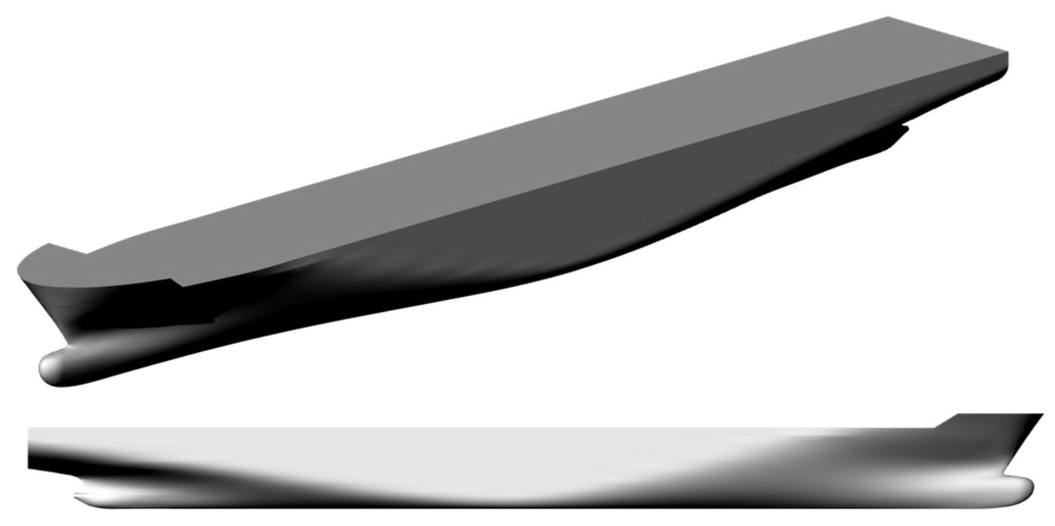
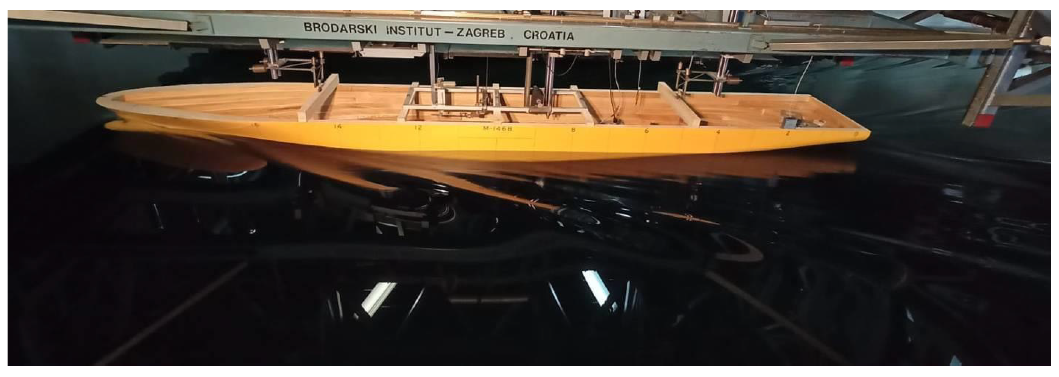
2. Containership and Propeller Characteristics

For this case study, a 6750-TEU containership was selected whose hull lines and 3D model are presented in Figure 1 and Figure 2, respectively. The main particulars of the containership at model and full scale are shown in

Table 1. The main particulars of the containership at the model and full scale.

Main Particular	Symbol	Unit of Measurement	Full Scale	Model Scale
Length between perpendiculars	LPP	m	286.58	8.1460
Length of waterline	LWL	m	292.37	8.3107
Breadth	B	m	40	1.1370
Draught at forward perpendicular	TF	m	11.98	0.3405
Draught at aft perpendicular	TA	m	11.98	0.3405
Draught at midship	TM	m	11.98	0.3405
Wetted surface area	S	m2	13,325	10.7668
Displacement volume	V	m3	85,556	1.9650
Longitudinal center of buoyancy (with respect to midship)	LCB	m	−5.07	−0.1440
Vertical center of buoyancy	ZCB	m	6.62	0.1882
Block coefficient	CB	-	0.6231
Midship section coefficient	CM	-	0.9850
Longitudinal prismatic coefficient	CP	-	0.6317
Waterplane area coefficient	CWP	-	0.7838

. The experiments with a ship model in a scale of 35.18 were carried out in the facility of the Brodarski Institute [30] in a 276 m long, 12.5 m wide, and 6 m deep towing tank, which is equipped with a towing carriage of maximum speed equal to 14 m/s.

The resistance, open water, and self-propulsion tests were conducted for a wide range of speeds. During the resistance tests, the model speed, total resistance, running trim, sinkage, and water temperature were measured.

During the self-propulsion tests, the ship model was equipped with a controllable pitch propeller (CPP) model,

Table 2. The main particulars of the propeller model.

Propeller Particulars	Symbol	Measurement Unit	V-1124 (CPP)
Diameter	D	m	0.2073
Pitch ratio at 0.7R	P0.7R/D	-	1.3
Expanded blade area ratio	AE/A0	-	0.633
Ratio of the hub diameter to the propeller diameter (hub ratio)	d/D	-	0.2957

.

The self-propulsion tests were performed based on the British method, meaning that the propeller load was varied at each speed, and propeller thrust, torque, and the propeller rate of revolution were measured along with the quantities measured in the resistance test. Self-propulsion tests were performed in a range of speeds from 16 knots to 22 knots that include conditions for slow steaming, i.e., the delivered power at the lowest tested speed was equal to one third of the delivered power at the highest speed.

The ship model during the self-propulsion test at the model speed corresponding to 22 knots in full scale is shown in Figure 3. The obtained experimental results were extrapolated based on the ITTC 1957 Performance Prediction Method using the correlation allowance equal to −0.35∙10⁻³. The required engine power at each speed was calculated based on the extrapolated value of the delivered power and an increase of 15% to account for the sea margin, 2% to account for the mechanical efficiency of transmission between engine and propeller, and 10% for engine margin.

3. Methodology

Once the propeller curve was determined, the two-stroke marine diesel engine was selected regarding the speed range and maximum brake power. The Wartsila Sulzer RTA-96C engine was selected based on the required brake power at 22 knots, as shown in Table 3. The measured data of engine performance and emissions declared by the engine manufacturer are defined according to ISO standard reference conditions. Engine variants with six, seven, and eight cylinders were considered a suitable choice based on the available data in the literature for containerships of a similar size. For the selected case study, the smallest variant of the selected engine type can propel the ship up to a speed of 23 knots. Usually, the design speed of containerships of similar size is around 25 knots. On the other hand, the engine with eight cylinders allows for sailing speeds up to 26 knots.

The 1D/0D simulation model of a six cylinder engine variant was made in AVL Boost™ [31] using the available geometry data from the manufacturer. The calibration of the simulation model was performed at 4 design operating points declared by the engine manufacturer, as illustrated in Figure 4. The simulation results of BMEP (brake mean effective pressure) and BSFC (brake specific fuel consumption) were compared with the reference engine data, achieving the deviation of simulation results within ±5% compared to the reference data of engine manufacturer.

Table 3. Specification of two-stroke marine diesel engine data and performance [32].

Engine Name	Wartsila Sulzer RTA-96C
Type	two-stroke diesel, turbocharged, liquid cooling
Scavenging type	unidirectional with exhaust valve
Fuel	MDF—marine diesel fuel (LHV = 42.7 MJ/kg)
Cylinder bore	960 mm
Piston stroke	2500 mm
Maximum engine speed	120 rpm
Maximum BMEP *	19.6 bar
Maximum brake power *	5490 kW per cylinder
BSFC at max. constant rating (at R1 operating point) * (ISO 3046-1) [33]	171 g/kWh
Cylinder arrangement and numbers (this study)	inline; 6, 7 and 8 cylinders

* ISO standard reference conditions: total barometric pressure 1.0 bar, suction air temperature 25 °C, charge air cooling–water temperature 25 °C, relative humidity 60%.

Table 3. Specification of two-stroke marine diesel engine data and performance [32].

Engine Name	Wartsila Sulzer RTA-96C
Type	two-stroke diesel, turbocharged, liquid cooling
Scavenging type	unidirectional with exhaust valve
Fuel	MDF—marine diesel fuel (LHV = 42.7 MJ/kg)
Cylinder bore	960 mm
Piston stroke	2500 mm
Maximum engine speed	120 rpm
Maximum BMEP *	19.6 bar
Maximum brake power *	5490 kW per cylinder
BSFC at max. constant rating (at R1 operating point) * (ISO 3046-1) [33]	171 g/kWh
Cylinder arrangement and numbers (this study)	inline; 6, 7 and 8 cylinders

* ISO standard reference conditions: total barometric pressure 1.0 bar, suction air temperature 25 °C, charge air cooling–water temperature 25 °C, relative humidity 60%.

At design operating points R1 and R3, the emission sub-model of nitrogen oxides was calibrated. The threshold of specific NO_X emissions is defined with Tier II regulation, which imposes that specific NO_X emissions should not exceed 14.4 g/kWh for engines with maximum speeds below 130 rpm. The additional calibration of the soot emission sub-model was made by simulating the engine load thatvaried from 5% to 100%. The 1D/0D simulation models are sensitive to the values of calibration parameters. Therefore, the reference engine performance and emission data should be used in the calibration steps. To correctly predict the engine performance and emissions in off-design conditions that are typical for slow steaming, the simulation model was calibrated at the design operating area.

By considering the engine performance defined by the manufacturer for different numbers of cylinders (from 6 up to 14), it is evident that BSFC and BMEP at R1 and R3 operating points are independent of the number of cylinders. Therefore, the engine performance with seven and eight cylinders was not simulated using the 1D/0D simulation model, but it was calculated by multiplying the engine brake power at each analyzed operating point with a factor that represents the relative increase in the number of cylinders compared to the power of an engine with six cylinders.

It is assumed that transition periods of ship acceleration and deceleration are very short compared to the total travel time, which means that instantaneous engine brake power is equal to the engine brake power required by the propeller. In other words, the instantaneous engine operating point lies on the propeller curve shown in Figure 4. The required power, ship speed, specific fuel consumption, and emissions can be evaluated for an arbitrary engine speed using linear interpolation.

The analysis of the effect of slow steaming on emissions of CO₂, NO_X and soot is performed for a typical Trans-Pacific route (4503 nm) for six-, seven- and eight-cylinder engines. The calculated operating costs, income per route and annual income represent the economic aspect of the application of slow steaming. Finally, the overall results of emissions for the seven- and eight-cylinder engines, costs and income are compared to the results for the 6-cylinder engine operating at the speed of 102 rpm.

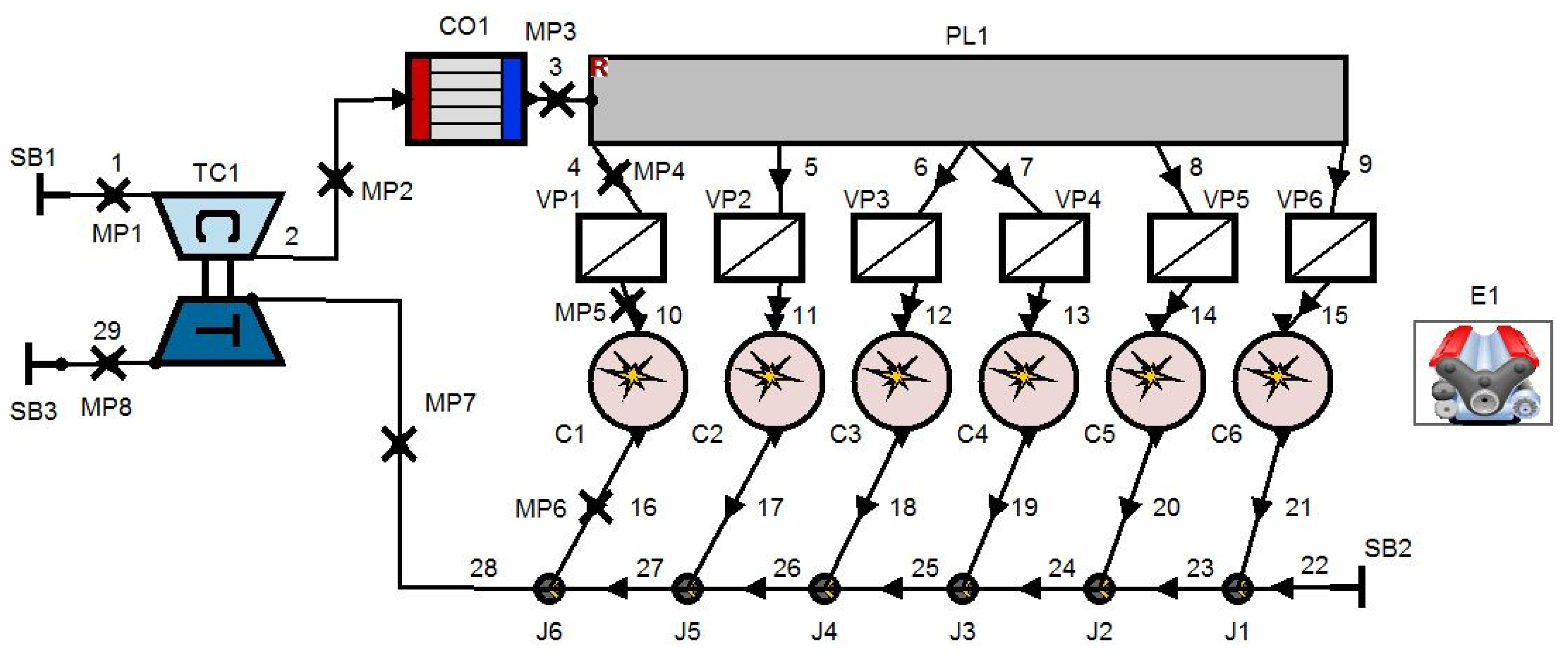
3.1. Engine Simulation Model

The 1D/0D simulation model of a six-cylinder two-stroke marine diesel engine is made in AVL Boost™, as shown in Figure 5. The model consists of a turbocharger (TC1), intake air cooler (CO1), intake plenums (PL1 and VP), cylinders (C1–C6), and exhaust pipes.

The intake system boundary (SB1) defines the intake boundary condition of pressure and temperature set to 0.98 bar and 25 °C, respectively. On the other hand, the exhaust boundary condition (SB2) of pressure is set to 0.98 bar, while the temperature is set to 225 °C. Such specification of boundary conditions represents the reduced engine intake and exhaust system without detailed modeling of filters, plenums, aftertreatment systems, etc. A simplified model of the turbocharger is used in which the turbocharger discharge coefficient is calculated to satisfy the desired pressure ratio at the compressor. At the engine speed of 102 rpm and BMEP of 19.6 bar (R1 operating point), the calculated boost pressure is equal to 3.7 bar. The excess air ratio is set to 1.6 at maximum loads and it increases as the engine load decreases. The combustion process is described using a two-zone Vibe function. A two-zone combustion model formulation means that in-cylinder mass during the combustion process consists of burned and unburned zones, creating better conditions for pollutant calculation, especially NO_X. The start of combustion is set to 5° crank angles after the Top Dead Center (TDC) at maximum engine speed according to manufacturer data regarding fuel injection timing [32]. The shape parameter and combustion duration of the Vibe function are set to 0.6 and 35° crank angles, respectively. The combustion model parameters are selected because the engine has 3 diesel fuel injectors per cylinder that intensify in-cylinder swirling, mixture formation, and hence the combustion burning rate is increased. The in-cylinder heat transfer is calculated using the well-known Woschni correlation, while the maximum temperature of the piston top surface is set to 380 °C as measured by the manufacturer [32]. The cylinder head temperature is set to 370 °C, while the cylinder liner temperature at TDC is equal to 285 °C and it decreases to BDC (bottom dead center) to 240 °C.

NO_X emissions are calculated considering six reactions that are based on the Zeldovich mechanism. More detail about reaction rates (r₁ − r₆) and coefficients (k_0,1 − k_0,6) using the Arrhenius-type form can be found in [34].

The soot emission is considered by calculating the soot formation and oxidation mechanism [35]. A soot formation reaction is related to the combustion rate of diffusion combustion $\frac{{\mathrm{d}m}_{\mathrm{fb},\mathrm{diff}}}{\mathrm{d}t}$ as follows:

$$\frac{{\mathrm{d}m}_{\mathrm{soot},\mathrm{f}}}{\mathrm{d}t}=A_{\mathrm{s},\mathrm{f}}·\frac{{\mathrm{d}m}_{\mathrm{fb},\mathrm{diff}}}{\mathrm{d}t}{·\left(\frac{p}{p_{\mathrm{ref}}}\right)}^{{\mathrm{n}}_1}·e^{\frac{E_{\mathrm{s},\mathrm{f}}}{R_{m}T}}$$

(1)

where A_s,f is the soot formation tuning parameter, p is the actual in-cylinder pressure, p_ref is the reference pressure, and E_s,f is the activation energy for soot formation. The soot oxidation reaction depends on the actual soot mass in the cylinder and available oxygen in the burned zone:

$$\frac{{\mathrm{d}m}_{\mathrm{soot},\mathrm{o}}}{\mathrm{d}t}=A_{\mathrm{s},\mathrm{o}}·\frac{1}{{\tau }_{\mathrm{char}}}·m_{\mathrm{soot}}^{{\mathrm{n}}_2}{·\left(\frac{p_{\mathrm{O}2}}{p_{\mathrm{O}2,\mathrm{ref}}}\right)}^{{\mathrm{n}}_3}·e^{\frac{E_{\mathrm{s},\mathrm{o}}}{R_{m}T}}$$

(2)

where A_s,o is the soot oxidation tuning parameter, τ_char is the characteristic mixing time related to the overall heat release rate, m_soot is the actual soot mass, p_O2 is the partial pressure of oxygen, p_O2,ref is the reference partial pressure of oxygen, and E_s,o is the activation energy for soot oxidation. In Equations (1) and (2), R_m and T are the individual gas constant and the temperature of the burned zone, respectively. In addition, n₁, n₂, and n₃ are model constants.

Once the simulation model was calibrated, the simulation results at reference operating points (design operation) were validated. After that, the simulation model was used to simulate the engine performance in off-design conditions (engine speed range 22–120 rpm and load range from 2.5% to 100%).

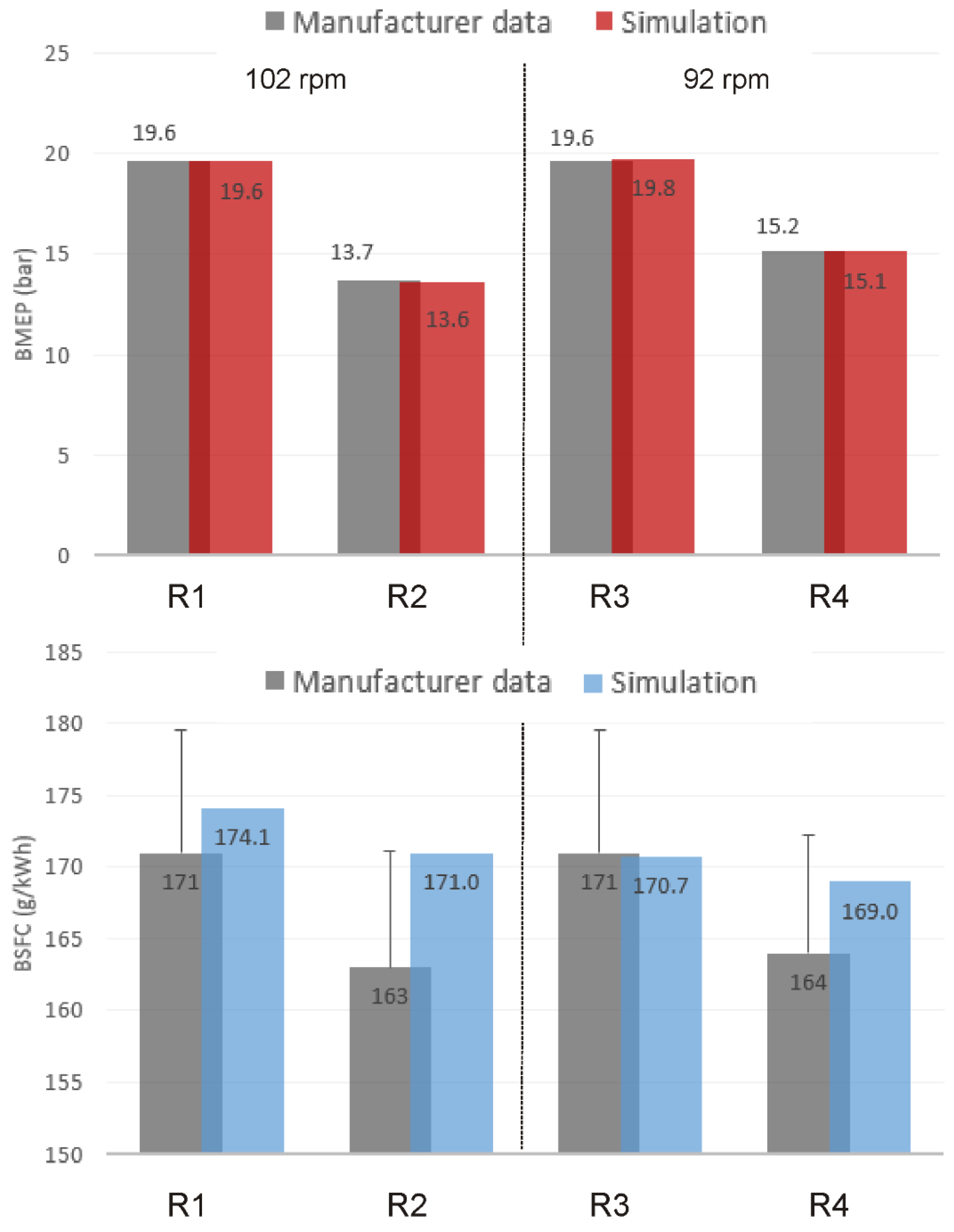
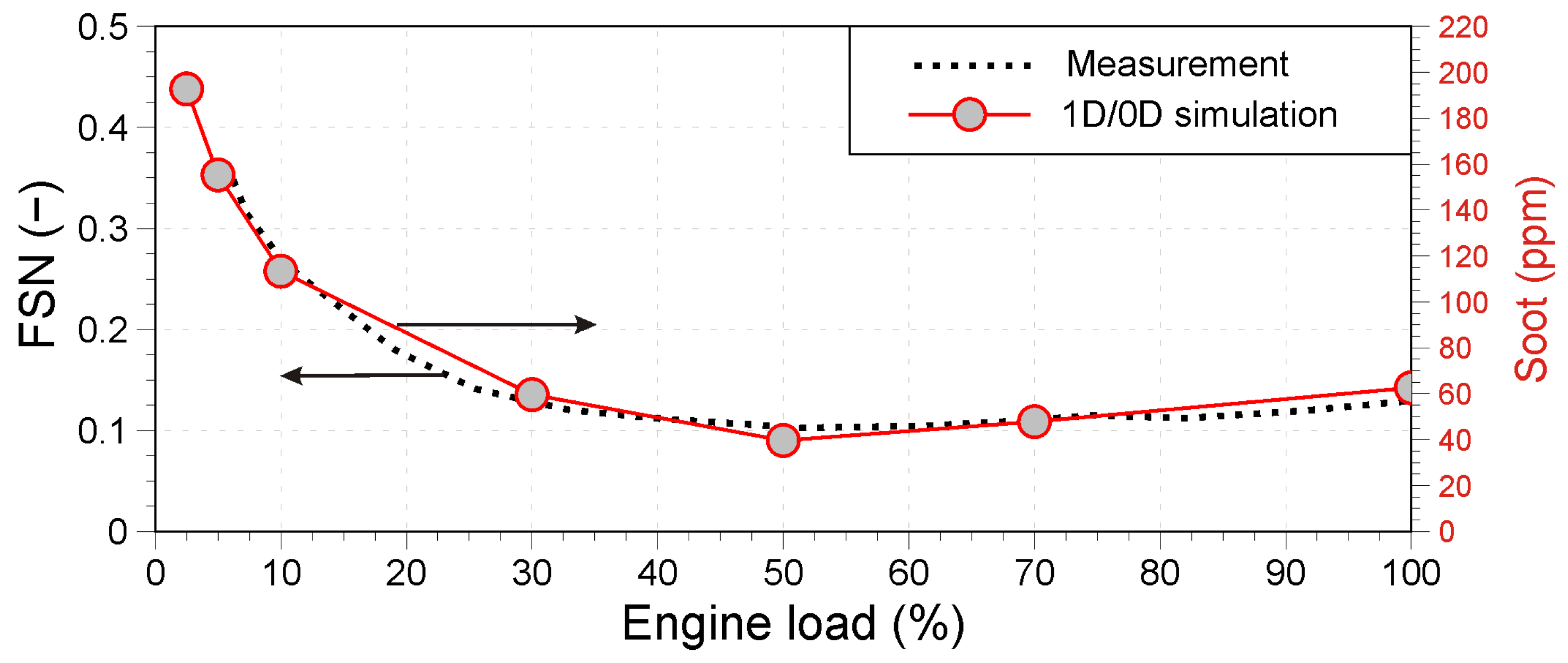
3.2. Validation of 1D/0D Simulation Model

The validation of the simulation model was performed by comparing the simulation results with engine performance data declared by the engine manufacturer. Figure 6 shows the comparison of BMEP and BSFC at four operating points (R1—full load at 102 rpm, R2—70% of load at 102 rpm, R3—full load at 92 rpm, and R4—load equal to R2 at 92 rpm).

During the model calibration process, several additional parameters are controlled. For example, the peak cylinder pressure is controlled by reaching a maximum value of 156 bar, the maximum fuel mass injected per cycle at 102 rpm is equal to 160 g and the boost pressure approximately is equal to 3.7 bar. Once the mentioned parameters were matched in the simulation model with a deviation of ±5%, the fine model tuning was performed. It includes the adoption of a heat transfer calibration factor for the piston, cylinder liner, and head to a value of 0.1, enabling the prediction of BSFC values within the deviation range of ±5% from the declared data, as shown in Figure 6. The comparison of the simulation results of BMEP and BSFC shown in Figure 6 confirms that the simulation model is validated in 4 different operating points (design engine operation), and it is applied to simulate the operation in off-design conditions. Before that, the soot emission results were compared over different engine loads at a reference engine speed of 102 rpm, Figure 7. The data measured by the manufacturer of soot emission are represented with values of Filter Smoke Number (FSN), while the simulation results are related to the soot mass ratio expressed in ppm units. To achieve simulation results of soot emission that increases as the engine load decreases, the soot formation parameter was calibrated and calibrated values that depend on engine load were applied for the simulation of other engine operating points. The soot oxidation parameter was kept at the default value.

The simulation results of soot emission matched the reference measured data of FSN well. As the engine load decreases, more soot is emitted because the lower boosting pressure is applied, reducing the quality of cylinder scavenging and turbulence quantities that are responsible for primary and secondary fuel break-up and the fuel/air mixing process.

The NO_X emission sub-model has two constants that can be modified during the calibration steps. The first constant named NO_X Kinetic Multiplier was set to the default unit value, while the NO_X Postprocessing Multiplier was increased from the default value of 0.64 to 0.80 so that the maximum NO_X emissions at R1 and R3 operating conditions do not exceed the threshold of 14.4 g/kWh, as defined by Trier II standard for ship engines with rotational speeds below 130 rpm.

4. Results and Discussions

4.1. Fuel Consumption and Emissions

Once the simulation model of the selected two-stroke marine diesel engine was calibrated, it was applied to simulate the off-design operating range. Topographic diagrams of BSFC, NO_X and soot emission are given in Figure 8, Figure 9 and Figure 10.

Ten engine speeds in the range from 22 rpm to 120 rpm are simulated, and at each engine speed, seven loads are analyzed, corresponding to 2.5%, 5%, 10%, 30%, 50%, 70% and 100% of the full load referenced at each engine speed. It means that 70 operating points were simulated, representing the overall engine operating range that includes design and off-design conditions.

BSFC is calculated so that the total fuel flow is divided by the engine brake power. When the engine power is lower, the mechanical losses become dominant in the total energy balance and therefore the BSFC increases significantly.

The engine power required by the propeller is also shown in Figure 8, Figure 9 and Figure 10. Since the transitional times of the propeller usually last for short periods while changing rotational speed, the engine operating points are positioned on the propeller curve. In other words, the equilibrium state between the engine and propeller is assumed.

The maximum values of specific emissions of NO_X are achieved at maximum engine loads when the maximum peak in-cylinder temperatures are reached. The NO_X model is calibrated so that the specific NO_X emissions at R1 and R3 operating points do not exceed values of 14.4 g/kWh, as limited by Tier II regulation standards for ship engines with rotational speed below 130 rpm. Since the two-zone combustion model formulation is used in this study, the main parameter responsible for the calculated NO_X emissions is the burned zone temperature. It can be seen from Figure 9 that a reduction in engine speed below 70 rpm will reduce NO_X emissions more than twice compared to the operating point at 102 rpm, where the maximum sailing speed of 23 knots will be achieved for the six-cylinder engine variant.

The specific soot emissions, shown in Figure 10, are calculated after the soot emission model is calibrated with reference data at 102 rpm, as already shown in Figure 7. The main characteristic of a marine two-stroke diesel engine is that soot emissions increase as the engine load decreases. Since the two-stroke marine diesel engine considered has unidirectional scavenging that mainly depends on the intake port pressure, an increased soot emission at a low engine load is caused by the increased residual gas concentration and lower in-cylinder turbulence intensity (lower flow velocities at intake port sectional area). The applied soot emission model used in this study does not include details about residual gas concentration and turbulence quantities and therefore the calibration of the soot formation parameter was required.

4.2. Engine Configuration with Six, Seven and Eight Cylinders

Considering the engine data declared by the manufacturer, the BMEP that is achieved at the R1 and R3 operating points is fully independent of the number of cylinders. This means that the brake engine power is proportional to the number of cylinders and the maximum engine power for the engine with seven and eight cylinders can be easily computed so that the brake power of the six-cylinder engine variant is multiplied by 7/6 and 8/6, respectively. Topographic diagrams of fuel consumption, NO_X and soot for seven- and eight-cylinder engine variants are generated so that the engine power at each operating point is multiplied by 7/6 and 8/6, respectively, while the property of fuel consumption and emissions expressed as specific values remain unchanged. The increase in maximum engine brake power increases the achievable maximum sailing speed. With a seven-cylinder engine variant, the maximum engine speed is equal to 110 rpm (speed of 25 knots), while the maximum engine speed of 116 rpm (speed of 26 knots) can be achieved with the eight-cylinder engine variant. The engine performance for operating points that are positioned at the propeller curve is calculated using linear interpolation.

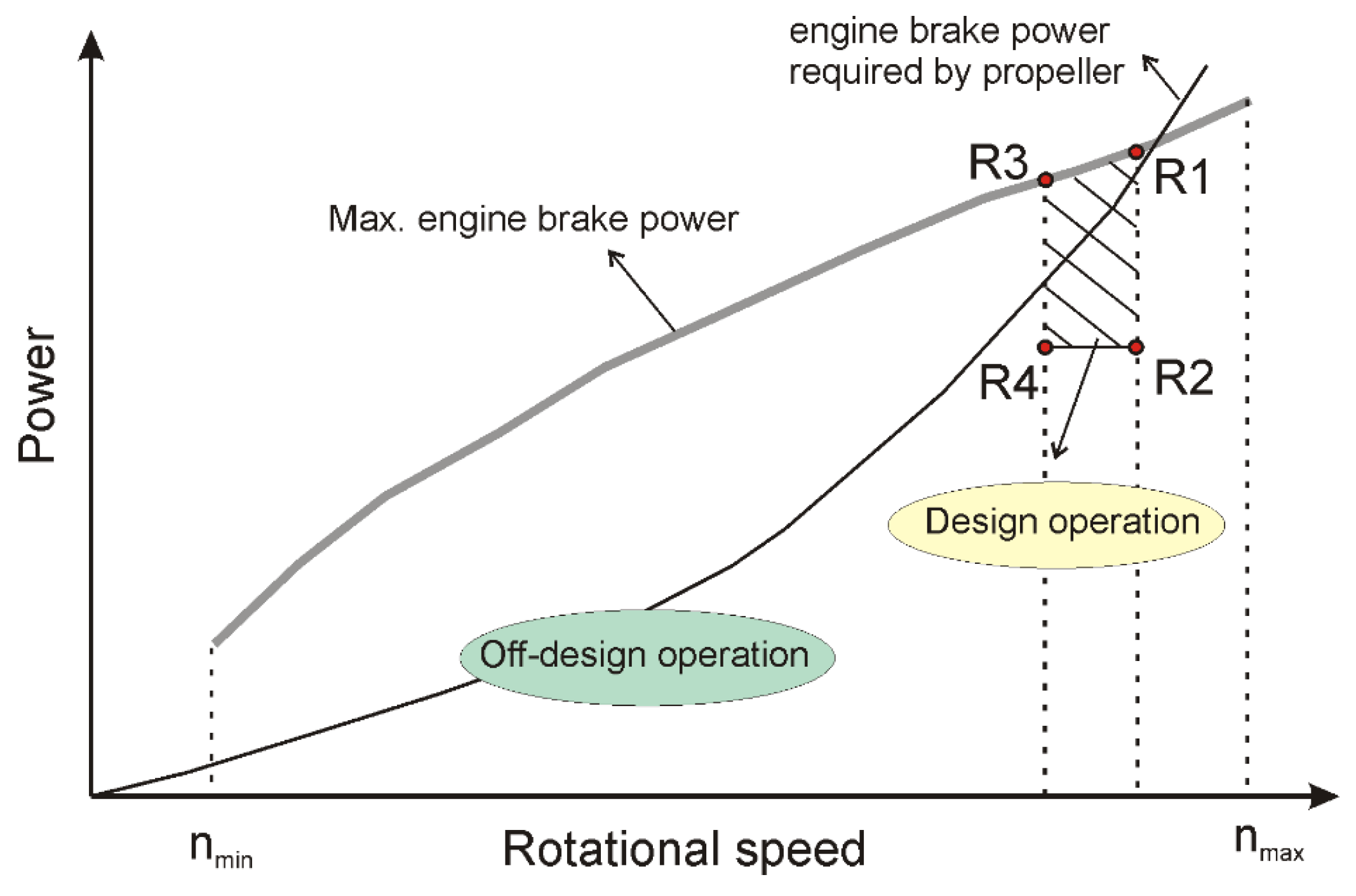
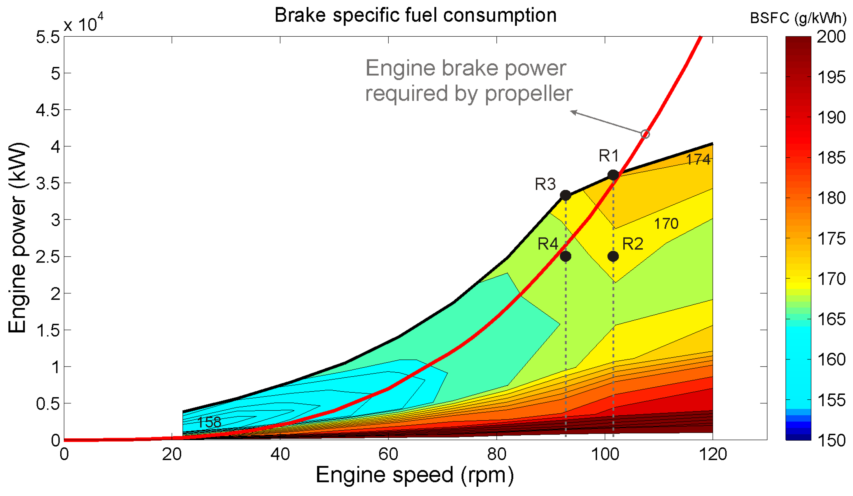
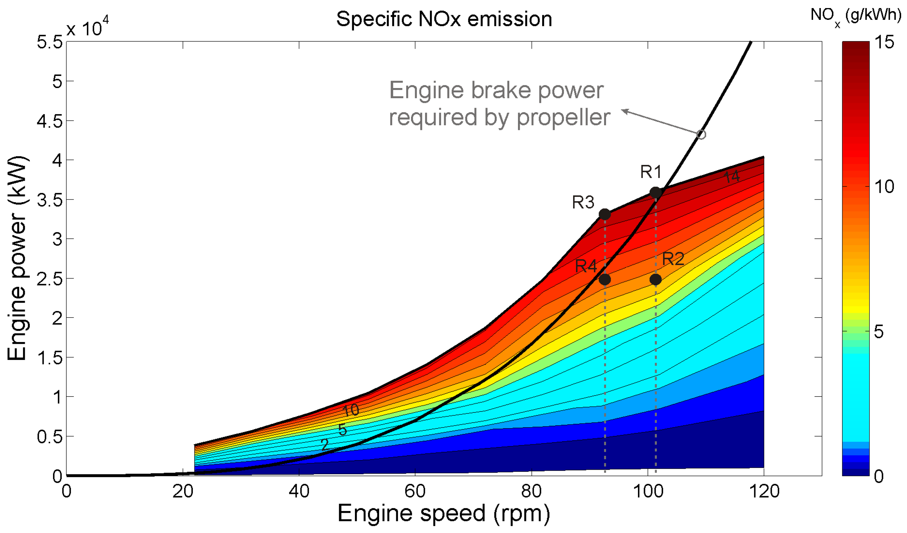
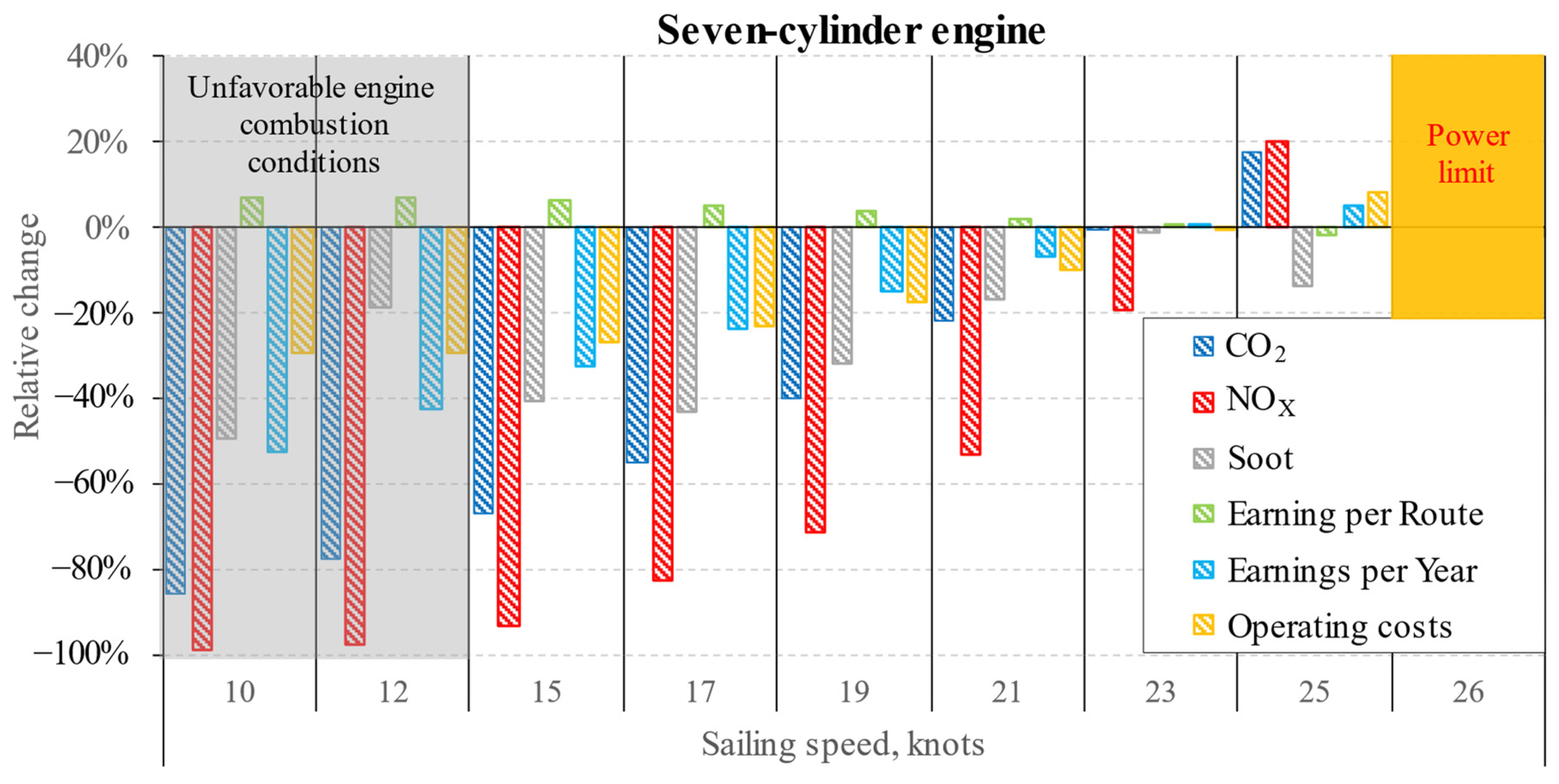
4.3. Off-Design Conditions

To determine the suitable engine variant under the slow steaming for the analyzed containership, an analysis of CO₂, NO_X, soot emissions, operating costs, annual incomes, and incomes per route was conducted. Figure 11, Figure 12 and Figure 13 provide an overview of the simulation results for CO₂, NO_X and soot emissions for simulated engine variants and engine speeds which correspond to sailing speeds from 10 to 26 knots. CO₂ emissions correspond to BSFC and fuel consumption, which depends on the engine load and in-cylinder conditions. Therefore, the CO₂ emissions decrease with sailing speed up to a certain speed, at which point the trend changes. The six-cylinder engine variant could not provide the required power at sailing speeds of 25 and 26 knots nor could the seven-cylinder engine variant at the speed of 26 knots. Each engine variant has minimum CO₂ emission at different sailing speeds. For a six-cylinder engine variant, the minimum of 508.2 g/kWh is achieved at 10 knots (42 rpm). The minimum for a seven-cylinder engine variant (509.23 g/kWh) is achieved at 12 knots (52 rpm), and for an eight-cylinder engine variant (509.86 g/kWh), it is also achieved at 12 knots. The minimum CO₂ emission is achieved with a six-cylinder engine variant because more favorable in-cylinder conditions and higher load conditions at low engine speeds are achieved. At sailing speeds below 12 knots, lower CO₂ emissions are achieved with engine variants with a lower number of cylinders, but above 12 knots, the trend changes. At higher speeds, favorable conditions for more efficient combustion, i.e., lower BSFC values, as shown in Figure 8, are achieved in engine variants with a greater number of cylinders.

The NO_X emissions decrease with the decrease in sailing and engine speeds, which is expected because NO_X emissions are highly dependent on in-cylinder temperature conditions, as shown in Figure 12. The minimum value is achieved at the lowest sailing speed (10 knots) with the eight-cylinder engine variant (0.57 g/kWh). At that operating point, the eight-cylinder engine variant has the lowest load and the lowest in-cylinder temperature. Soot emissions show the opposite trend compared to NO_X emissions.

With the reduction in sailing speed, the soot emissions increase (see Figure 13) because the unfavorable in-cylinder mixing conditions caused by lower boost pressure and in-cylinder turbulence intensity are achieved. An indicator of a less favorable combustion behavior, which could lead to higher repair and maintenance costs, is a large gradient in the specific soot emission. Keeping that in mind, the sailing speed for six-cylinder and seven-cylinder engine variants could be limited to 12 knots (engine speed of 52 rpm) and that for the eight-cylinder engine variant to 15 knots (engine speed of 62 rpm).

The confirmation for such criteria is that the relative increase in specific soot emissions of 95.5% in the case of the six-cylinder engine variant is observed in the sailing speed reduction from 15 to 12 knots. For the seven-cylinder engine variant, the relative increase in specific soot emission of 97.7% is also observed in the sailing speed reduction from 15 to 12 knots. For the eight-cylinder engine variant, the relative increase in specific soot emissions of 91.2% is observed in the sailing speed reduction from 17 to 15 knots.

In addition to emissions, slow steaming also affects the operating costs. During slow steaming, the fuel costs are reduced and, due to longer sailing time, the crew costs are increased. Changes in operating costs consequently change the ship’s income. The effects of sailing speed on operating costs, income per route and annual income are shown in Figure 14, Figure 15 and Figure 16. The costs and income were analyzed for the Trans-Pacific route (4503 nm). According to [36], the average contract freight rate for a 40-foot container or 40-foot equivalent unit (FEU) on the route from Asia to North America is 2580 USD/FEU. The ship is designed to carry 6750 TEU, which is equal to 3375 FEU and represents a cargo value of USD 8,707,500.00. The reference ship marine engine is the six-cylinder engine variant. As each new cylinder section of the Wartsila Sulzer RTA-96C engine series adds additional weight, the seven-cylinder engine variant has 130 tons more weight [37], which is the weight of 5 TEU and the carrying capacity for the seven-cylinder engine variant is 6745 TEU. The eight-cylinder engine variant has 300 tons more than the six-cylinder engine variant, which means that the carrying capacity of the eight-cylinder engine variant is 6738 TEU. That represents a decrease in cargo value of 0.07% and 0.18% for the ship configuration with the seven-cylinder and eight-cylinder engine variants, respectively. In general, the operating costs are comprise fuel costs, port charges, crew costs, repair and maintenance costs, insurance charges, parts and lubes costs, and administration costs [38]. According to the diagram which depicts the distribution of operating costs of Panamax, Post Panamax and Post Panamax plus containerships sourced from Drewry Shipping Consultants Ltd., London, United Kingdom in [38], in the case of a Post Panamax containership, the fuel contributes to 49% of operating costs, port charges to 23%, insurance charges to 8%, repair and maintenance costs to 8%, stores and lubes to 2%, manning or crew costs to 8%, and administration to 2%. The fuel costs and overall operating costs were calculated based on the global 20 ports’ average price of Very Low Sulfur Fuel Oil (VLSFO), also known as IMO2020 grade bunkers, which is currently 658 USD/ton [39]. The operating costs for all engine configurations are calculated based on the assumption that 49% of operating costs are fuel costs and all other operating costs are calculated according to their above-mentioned contribution to overall operating costs. The reference operating costs are calculated for the sailing speed of 23 knots at which the ship can sail the selected route in 195.5 h. Insurance charges, repair and maintenance costs, stores and lubes costs and administrative costs are assumed independent on sailing time and frequency and these costs are set to constant values. Crew costs are calculated by multiplying the required sailing time and the crew costs per hour.

The crew cost per hour (825.3 USD/hour) is calculated by dividing the reference crew cost (161,363.75 USD/route) by the reference sailing time (195.5 h). The operating costs decrease with the reduction in sailing speed, as can be seen in Figure 14. The reduction in operating costs is the result of lower fuel consumption in the analyzed operating range of the engine. At the reference sailing speed (23 knots), the six-cylinder engine variant has the highest operating costs (USD 1,457,491.47) because the highest fuel consumption is reached. On the other hand, the eight-cylinder engine variant works at the most efficient engine operating point, resulting in the lowest operating costs (USD 1,453,675.24).

The operating costs decrease with the increase in the number of cylinders at sailing speeds of 19, 21, and 23 knots. At lower sailing speeds, the differences between the operating costs for different engine variants are negligible. The decrease in operating costs results in an increase in ship income per route, as shown in Figure 15. Due to longer sailing time, less cargo can be transported in one year and therefore the annual income decreases significantly with the reduction in sailing speed, as shown in Figure 16.

Relative changes in emissions, operating costs, income per route and annual incomes with sailing speed for all three engine variants compared to the six-cylinder engine variant at the design speed of 23 knots are shown in Figure 17, Figure 18 and Figure 19. The annual incomes are calculated assuming the same ship sailing route for the entire year.

The lowest sailing speed is determined as the speed at which the specific soot emissions significantly increase, as shown in Figure 13. For the six- and seven-cylinder engine variants, the engine can be safely operated up to a sailing speed of 15 knots, and for the eight-cylinder engine variant, up to 17 knots. With a higher number of cylinders, the NO_X emissions significantly decrease, i.e., 19.7% in the case of the seven-cylinder engine variant and 34.5% in the case of the eight-cylinder engine variant. This occurred because lower engine loads in the seven- and eight-cylinder engine variants and consequently lower in-cylinder temperatures are achieved. For all engine variants and sailing speeds below the reference one, CO₂ emissions can be reduced by up to 67.2%, NO_X emissions up to 93.3% and soot emissions up to 53.4%. The same is true for operating costs, where the largest reduction of 27.13% can be achieved with the seven-cylinder engine variant. The largest reduction in operating costs in the case of the six-cylinder engine variant is 27.1%, and in the case of the eight-cylinder engine variant, 23.18%. The income per route slowly increases with the decrease in sailing speed. The highest feasible increase in ship income per route is 6.16% and it is achieved with the six-cylinder engine variant at a sailing speed of 15 knots. With the seven-cylinder engine variant, the highest achievable increase in income per route is 6.08%, and with the eight-cylinder engine variant, 5.06%. The annual income decreases with sailing speed up to 32.84% in the case of the seven-cylinder engine variant and at a sailing speed of 15 knots. The decrease in annual income in the case of the six-cylinder engine variant is up to 32.79%, and in the case of the eight-cylinder engine variant, 23.73%. The smallest decrease in annual income in the case of the eight-cylinder engine variant is because the lowest achievable sailing speed is 17 knots. Also, with the increase in sailing speed, the annual income can increase 8.58% above the reference value in the case of the eight-cylinder engine variant, but in that case, the CO₂ emissions would increase by 32.8%. In 2023, IMO introduced a new measure to reduce the carbon intensity of existing ships, the EEXI. It requires ships to meet certain emission targets based on their size, type, and age, at their next annual, intermediate, or renewal survey after January 1st 2023. The aim is to achieve a 40% reduction in carbon emissions by 2030 compared to 2008 levels. The EU introduced a package of legislative proposals called Fit for 55, which also includes the reform of the EU ETS. It aims to achieve a 55% reduction in GHG emissions by 2030 compared to 1990 levels.

To comply with the regulations, in the case of the six- and seven-cylinder engine variants, the lowest sailing speed is equal to 15 knots, and for the eight-cylinder engine variant, it is equal to 17 knots, as shown in Figure 20.

In the case of a sailing speed of 17 knots, the eight-cylinder engine variant is the only one that complies with EU legislative requirements, but the differences are in the range of 1%. The decrease in the sailing speed to 17 knots results in an annual income decrease of around 24% compared to the reference engine variant and sailing speed. To maximize the income per route, the most suitable sailing speed is 15 knots with the six-cylinder engine variant, where the income per route increases by up to 6.2% and the CO₂ emissions decrease by up to 67.1%.

5. Conclusions

In this article, the goal was to investigate the influence of the two-stroke marine diesel engine variant on the selection of the most favorable slow steaming speed and its environmental and economic impact. This research was conducted on a case study of a Post Panamax containership with three different two-stroke marine diesel engine variants (six-cylinder, seven-cylinder and eight-cylinder engine). To select the sailing speed in slow steaming conditions, which would result in optimal correlation between reduced fuel costs, CO₂ emissions, NO_X emissions and increased operating costs in the frame of recent legislative measures to reduce GHG and NO_X emissions, the propeller-delivered power and engine performance and emissions must be estimated with a high level of accuracy. The propeller-delivered power–engine speed function required for the engine selection was experimentally determined based on the hydrodynamic characteristics of the selected ship and propeller and it defined the required engine brake power and engine speed. The marine two-stroke diesel engine was simulated using a comprehensive thermodynamic 1D/0D tool to predict the engine performance and emissions in design and off-design conditions. Engine variants with six, seven and eight cylinders were analyzed, and the effect of slow steaming on engine emissions and operating costs was quantified for one typical Trans-Pacific route. For the analyzed containership and propeller, the maximum sailing speeds of 23 knots, 25 knots, and 26 knots can be achieved with the engine variants with six, seven, and eight cylinders, respectively.

The case study investigated resulted in the following conclusions:

• The application of the 1D/0D simulation model and propeller-delivered power function can be a useful step for the calculation of ship engine performance and exhaust gas emissions in off-design conditions typical for slow steaming.
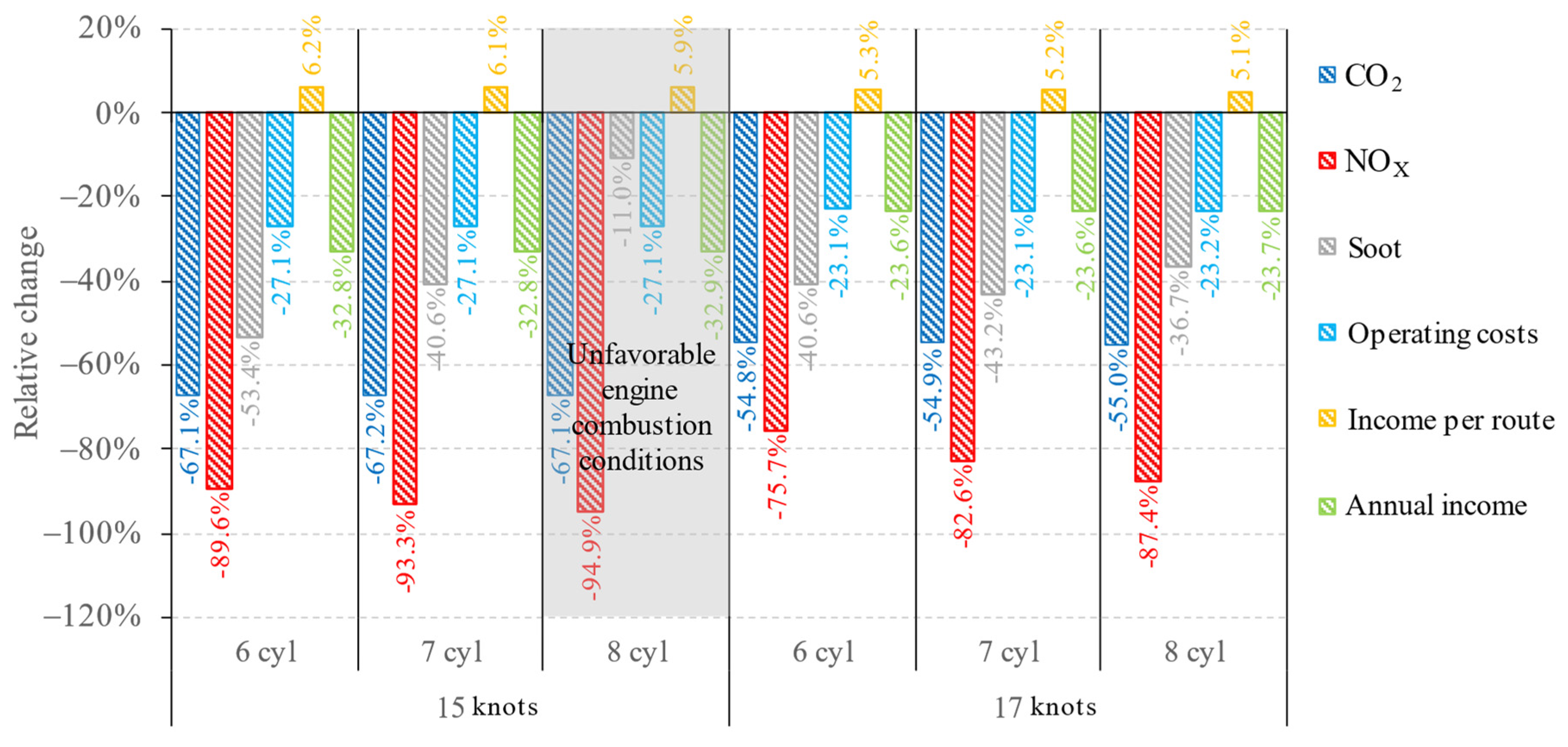
• The lowest engine speed, which the engine can safely sustain, varies between engine variants. The lowest achievable sailing speed for six-cylinder and seven-cylinder engines is 15 knots, and for the eight-cylinder engine, it is 17 knots.
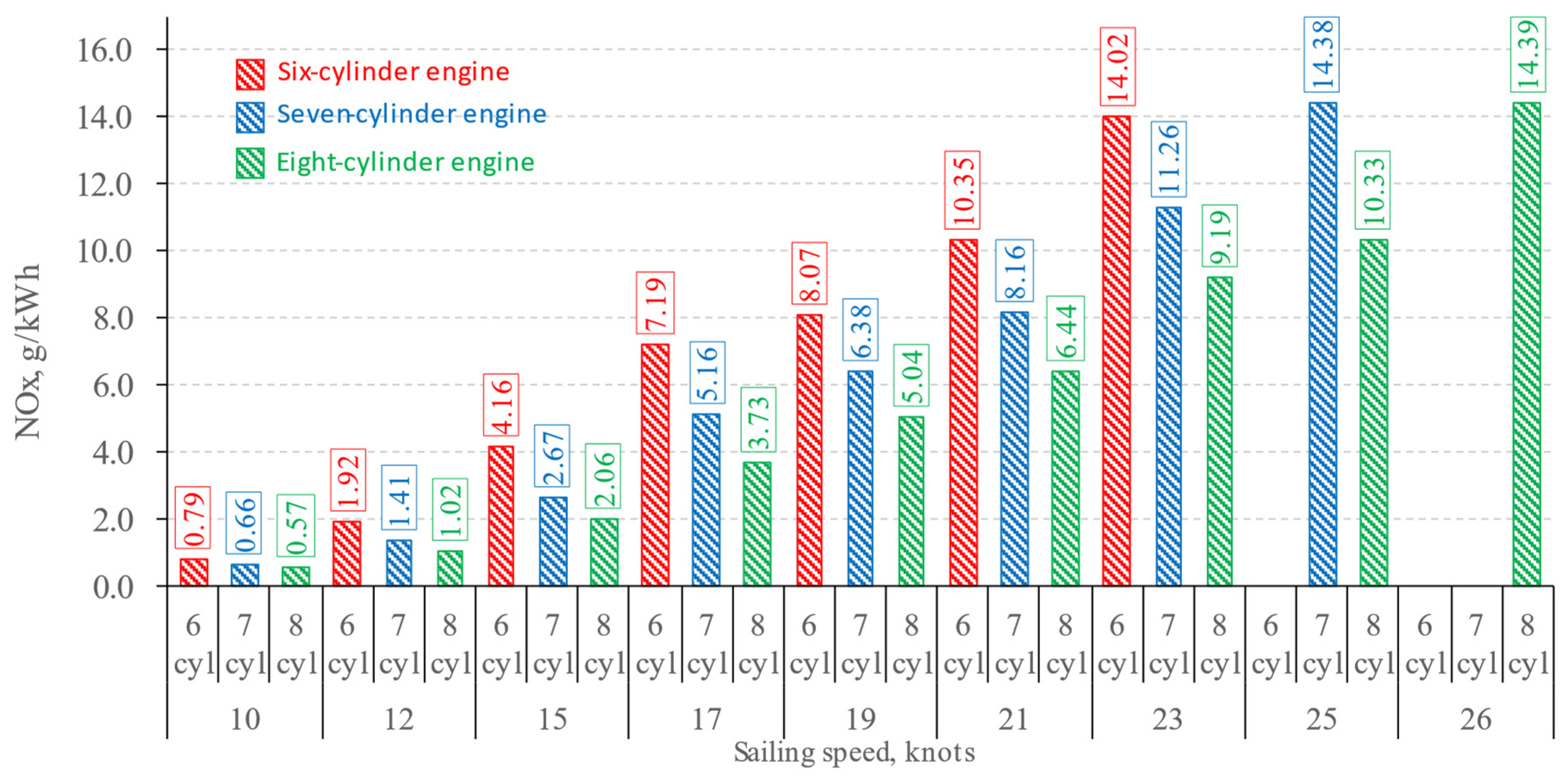
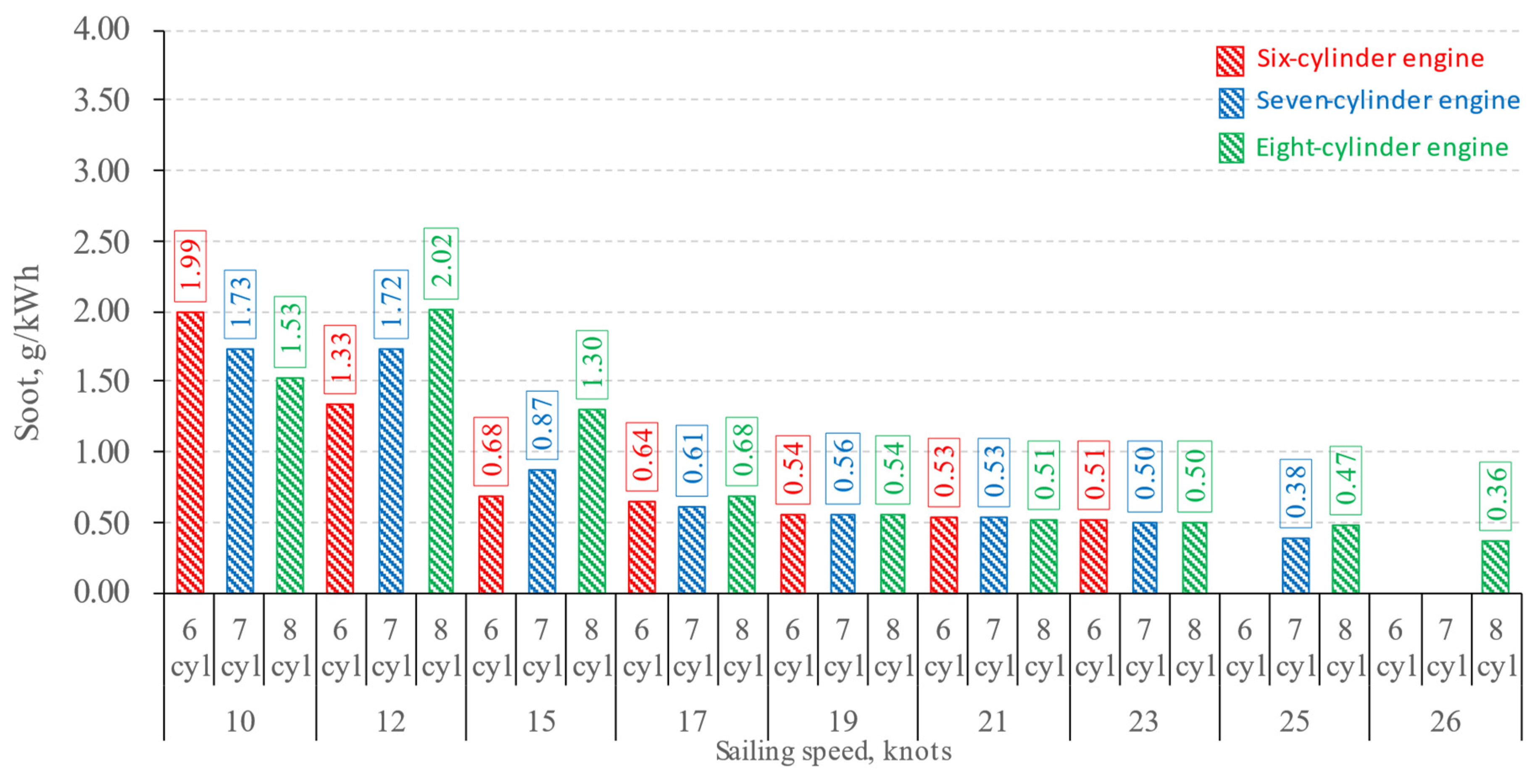
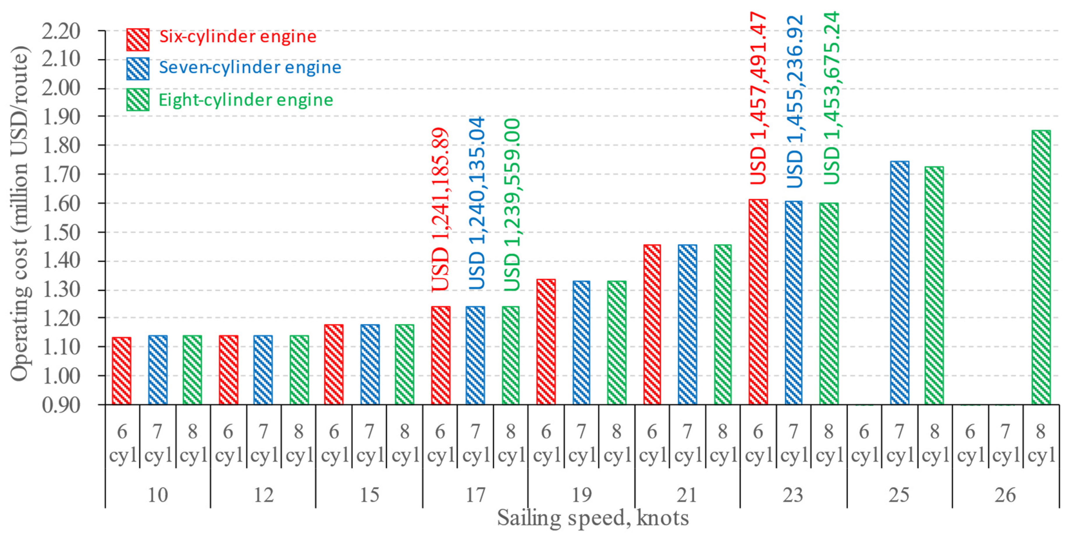
• The reduction in sailing speed by 35% (from 23 knots to 15 knots) for ship powered by the six-cylinder engine variant resulted in the reduction in CO₂, NO_X, and soot by 67.1%, 89.6% and 53.4%, respectively, and that engine variant provides the highest income per route.
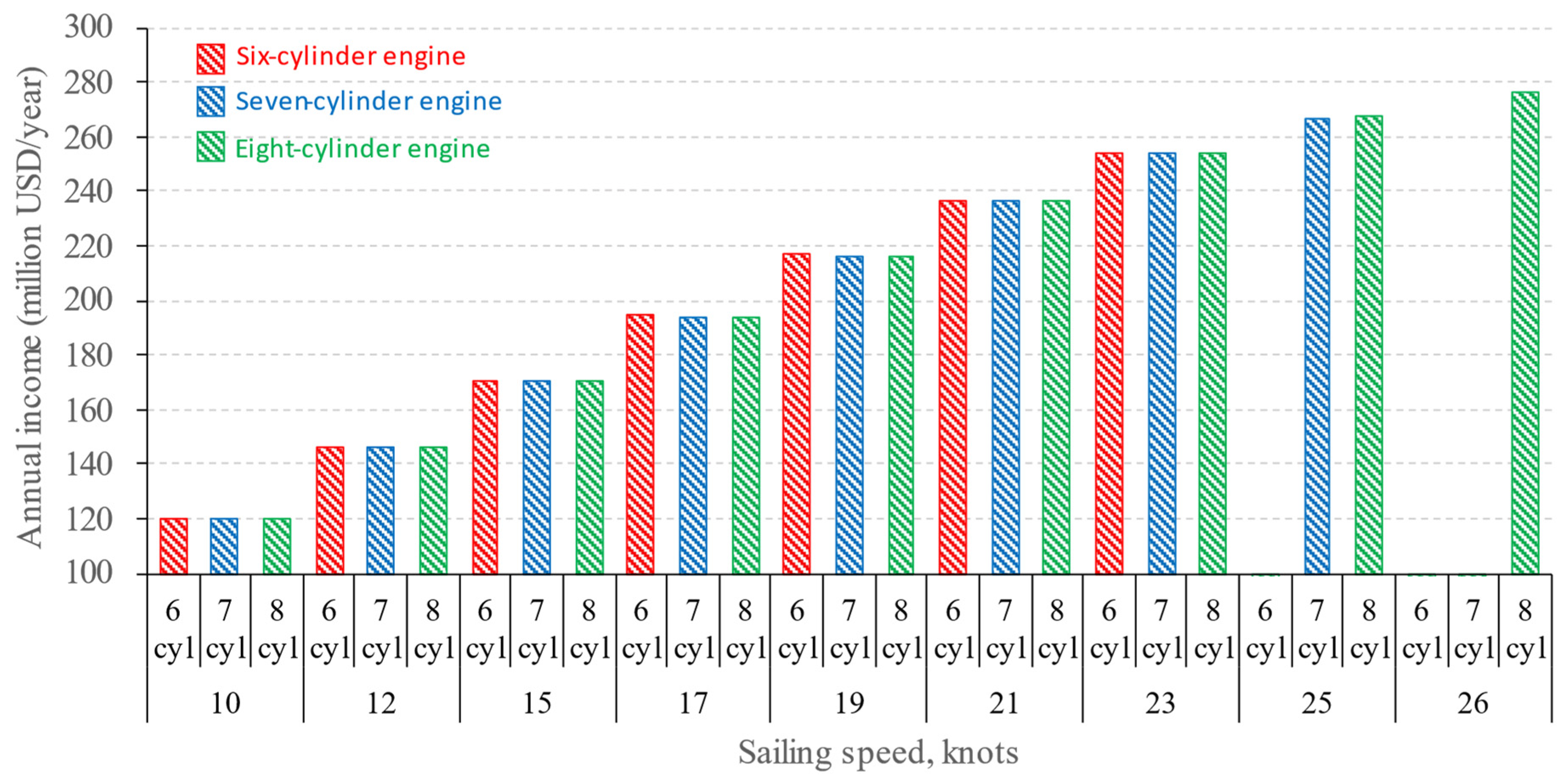
• The income for the analyzed Trans-Pacific route at the sailing speed of 15 knots is increased by 6.2%, while the annual income is decreased by 32.8% because a longer sailing time per route is required.
• To satisfy the targeted 55% reduction in GHG emissions by 2030 under slow steaming conditions, the sailing speed should be reduced by at least 26% compared to the design speed. Such a reduction can be achieved with all engine variants at sailing speed of 17 knots, in which case the eight-cylinder engine variant ensures the highest reduction in CO₂ emission (55%), NO_X emission (87.4%) and the highest annual income decrease (23.7%).

Future studies could be focused on the analysis of the environmental and economic impact of ship fleets, which includes different engine sizes, ship capacities and sailing routes. On the other hand, the application of alternative fuels such as natural gas, e-fuels and ammonia has great potential to reduce GHG emissions, especially under slow steaming, which could also be incorporated into the analysis.

References

1. International Maritime Organization. 2023 IMO Strategy on Reduction of GHG Emissions from Ships; Annex 1, Resolution MEPC.377(80); IMO: London, UK, 2023. [Google Scholar]
2. European Comission, Regulation (EU) 2023/957 of the European Parliament and of the Council. Available online: https://eur-lex.europa.eu/eli/reg/2023/957 (accessed on 18 February 2024).
3. Chua, Y.J.; Soudagar, I.; Ng, S.H.; Meng, Q. Impact analysis of environmental policies on shipping fleet planning under demand uncertainty. Transp. Res. D Transp. Environ. 2023, 120, 103744. [Google Scholar] [CrossRef]
4. Tuswan, T.; Sari, D.P.; Muttaqie, T.; Prabowo, A.R.; Soetardjo, M.; Murwantono, T.T.P.; Utina, R.; Yuniati, Y. Representative application of LNG-fuelled ships: A critical overview on potential GHG emission reductions and economic benefits. Brodogradnja 2023, 74, 63–83. [Google Scholar] [CrossRef]
5. Dotto, A.; Satta, F.; Campora, U. Energy, environmental and economic investigations of cruise ships powered by alternative fuels. Energy Convers. Manag. 2023, 285, 117011. [Google Scholar] [CrossRef]
6. Bayraktar, M.; Yuksel, O. A scenario-based assessment of the energy efficiency existing ship index (EEXI) and carbon intensity indicator (CII) regulations. Ocean Eng. 2023, 278, 114295. [Google Scholar] [CrossRef]
7. Horvath, S.; Fasihi, M.; Breyer, C. Techno-economic analysis of a decarbonized shipping sector: Technology suggestions for a fleet in 2030 and 2040. Energy Convers. Manag. 2018, 164, 230–241. [Google Scholar] [CrossRef]
8. Xing, H.; Spence, S.; Chen, H. A comprehensive review on countermeasures for CO2 emissions from ships. Renew. Sustain. Energy Rev. 2020, 134, 110222. [Google Scholar] [CrossRef]
9. United Nations. Review of Maritime Transport. Available online: https://unctad.org/system/files/official-document/rmt2023_en.pdf (accessed on 18 February 2024).
10. Czermański, E.; Oniszczuk-Jastrząbek, A.; Spangenberg, E.F.; Kozłowski, L.; Adamowicz, M.; Jankiewicz, J.; Cirella, G.T. Implementation of the Energy Efficiency Existing Ship Index: An important but costly step towards ocean protection. Mar. Policy 2022, 145, 105259. [Google Scholar] [CrossRef]
11. Braidotti, L.; Bertagna, S.; Rappoccio, R.; Utzeri, S.; Bucci, V.; Marinò, A. On the inconsistency and revision of Carbon Intensity Indicator for cruise ships. Transp. Res. D Transp. Environ. 2023, 118, 103662. [Google Scholar] [CrossRef]
12. Godet, A.; Nurup, J.N.; Saber, J.T.; Panagakos, G.; Barfod, M.B. Operational cycles for maritime transportation: A benchmarking tool for ship energy efficiency. Transp. Res. D Transp. Environ. 2023, 121, 103840. [Google Scholar] [CrossRef]
13. Farkas, A.; Degiuli, N.; Martić, I.; Grlj, C.G. Is slow steaming a viable option to meet the novel energy efficiency requirements for containerships? J. Clean. Prod. 2022, 374, 133915. [Google Scholar] [CrossRef]
14. Marques, C.H.; Pereda, P.C.; Lucchesi, A.; Ramos, R.F.; Fiksdahl, O.; Assis, L.F.; Pereira, N.N.; Caprace, J.D. Cost and environmental impact assessment of mandatory speed reduction of maritime fleets. Mar. Policy 2023, 147, 105334. [Google Scholar] [CrossRef]
15. Finnsgård, C.; Kalantari, J.; Roso, V.; Woxenius, J. The Shipper’s perspective on slow steaming-Study of Six Swedish companies. Transp. Policy 2020, 86, 44–49. [Google Scholar] [CrossRef]
16. Wu, W.M. The optimal speed in container shipping: Theory and empirical evidence. Transp. Res. E Logist. Transp. 2020, 136, 101903. [Google Scholar] [CrossRef]
17. Kalajdžić, M.; Vasilev, M.; Momčilović, N. Power reduction considerations for bulk carriers with respect to novel energy efficiency regulations. Brodogradnja 2022, 73, 79–92. [Google Scholar] [CrossRef]
18. Tran, N.K.; Lam, J.S.L. Effects of container ship speed on CO2 emission, cargo lead time and supply chain costs. Res. Transp. Bus. 2022, 43, 100723. [Google Scholar] [CrossRef]
19. Farkas, A.; Degiuli, N.; Martić, I.; Mikulić, A. Benefits of slow steaming in realistic sailing conditions along different sailing routes. Ocean Eng. 2023, 275, 114143. [Google Scholar] [CrossRef]
20. Yu, H.; Fang, Z.; Fu, X.; Liu, J.; Chen, J. Literature review on emission control-based ship voyage optimization. Transp. Res. D Transp. Environ. 2021, 93, 102768. [Google Scholar] [CrossRef]
21. Berthelsen, F.H.; Nielsen, U.D. Prediction of ships’ speed-power relationship at speed intervals below the design speed. Transp. Res. D Transp. Environ. 2021, 99, 102996. [Google Scholar] [CrossRef]
22. Psaraftis, H.N.; Lagouvardou, S. Ship speed vs. power or fuel consumption: Are laws of physics still valid? Regression analysis pitfalls and misguided policy implications. Clean. Logist. Supply Chain 2023, 7, 100111. [Google Scholar] [CrossRef]
23. Lee, C.Y.; Lee, H.L.; Zhang, J. The impact of slow ocean steaming on delivery reliability and fuel consumption. Transp. Res. E Logist. Transp. 2015, 76, 176–190. [Google Scholar] [CrossRef]
24. Zincir, B. Slow steaming application for short-sea shipping to comply with the CII regulation. Brodogradnja 2023, 74, 21–38. [Google Scholar] [CrossRef]
25. Degiuli, N.; Martić, I.; Farkas, A.; Buča, M.P.; Dejhalla, R.; Grlj, C.G. Experimental assessment of the hydrodynamic characteristics of a bulk carrier in off-design conditions. Ocean Eng. 2023, 280, 114936. [Google Scholar] [CrossRef]
26. Zhang, F.; Chen, Y.; Su, P.; Cui, M.; Han, Y.; Matthias, V.; Wang, G. Variations and characteristics of carbonaceous substances emitted from a heavy fuel oil ship engine under different operating loads. Environ. Pollut. 2021, 284, 117388. [Google Scholar] [CrossRef] [PubMed]
27. Guan, C.; Theotokatos, G.; Zhou, P.; Chen, H. Computational investigation of a large containership propulsion engine operation at slow steaming conditions. Appl. Energy 2014, 130, 370–383. [Google Scholar] [CrossRef]
28. Di Natale, F.; Carotenuto, C. Particulate matter in marine diesel engines exhausts: Emissions and control strategies. Transp. Res. D Transp. Environ. 2015, 40, 166–191. [Google Scholar] [CrossRef]
29. Duan, K.; Li, Q.; Liu, H.; Zhou, F.; Lu, J.; Zhang, X.; Zhang, Z.; Wang, S.; Ma, Y.; Wang, X. Dynamic NOx emission factors for main engines of bulk carriers. Transp. Res. D Transp. Environ. 2022, 107, 103290. [Google Scholar] [CrossRef]
30. Brodarski Institute. Resistance, Self-Propulsion and 3D Wake Measurement Test Results; Report 6652-M; Brodarski Institute: Zagreb, Croatia, 2022. [Google Scholar]
31. AVL BOOST, version 2013. Computer software. AVL List GmbH: Graz, Austria, 2013.
32. Demmerle, R. Sulzer RTA-C, Technology Review—Sulzer RTA84C and RTA96C Engines: The Reliable Driving Forces for Large, Fast Containerships; Wärtsillä NSD Swizerland Ltd.: Winterthur, Switzerland, 1997. [Google Scholar]
33. ISO 3046-1:2002; Reciprocating Internal Combustion Engine—Performance, Part 1: Declarations of Power, Fuel and Lubrication Oil Consumption, and Test Methods—Additional Requirements for Engines for General Use. Edition 5; ISO: Geneva, Switzerland, 2002.
34. Sjerić, M.; Krajnović, J.; Vučetić, A.; Kozarac, D. Influence of Swirl Flow on Combustion and Emissions in Spark-Ignition Experimental Engine. J. Energy Eng. 2021, 147, 04021014. [Google Scholar] [CrossRef]
35. Schubiger, R.A.; Boulouchos, K.; Eberle, M.K. Rußbildung und Oxidation bei der dieselmotorischen Verbrennung. MTZ-Mot. Z. 2002, 63, 342–353. [Google Scholar] [CrossRef]
36. United Nations. Review of Maritime Transport. Chapter 3: Freight Rates, Maritime Transport Costs and Their Impact on Prices. 2021. Available online: https://unctad.org/system/files/official-document/rmt2021_en_0.pdf (accessed on 19 February 2024).
37. Bilousov, I.; Bulgarkov, M.; Savchuk, V. Modern Marine Internal Combustion Engines—A Technical and Historical Overview; Springer Nature: Cham, Switzerland, 2020; Volume 8, pp. 347–349. [Google Scholar]
38. The Geography of Transport Systems—Operating Costs of Panamax and Post-Panamax Containerships. Available online: https://transportgeography.org/contents/chapter5/maritime-transportation/containerships-operating-costs-panamax-post-panamax/ (accessed on 19 February 2024).
39. Ship & Bunker—Hong Kong Bunker Prices. Available online: https://shipandbunker.com/prices/apac/ea/cn-hok-hong-kong#VLSFO (accessed on 19 February 2024).
Figure 1. Hull lines of the 6750-TEU containership.
Applsci 14 04634 g001
Figure 2. Three-dimensional model of the 6750-TEU containership.
Applsci 14 04634 g002
Figure 3. Self-propulsion test at the speed corresponding to 22 knots in full scale.
Applsci 14 04634 g003
Figure 4. Definition of off-design engine operation and positions of calibration operating points R1-R4 declared by engine manufacturer.
Applsci 14 04634 g004
Figure 5. Simulation model of two-stroke diesel engine Wartsila Sulzer RTA-96C.
Applsci 14 04634 g005
Figure 6. Validation of simulation results with engine manufacturer data.
Applsci 14 04634 g006
Figure 7. Validation of soot emission results at 102 rpm.
Applsci 14 04634 g007
Figure 8. Diagram of BSFC for design and off-design operating range.
Applsci 14 04634 g008
Figure 9. Diagram of specific NOX emissions for design and off-design operating range.
Applsci 14 04634 g009
Figure 10. Diagram of specific soot emission for design and off-design operating range.
Applsci 14 04634 g010
Figure 11. The comparison of CO2 emissions for different engine variants at different sailing speeds.
Applsci 14 04634 g011
Figure 12. The comparison of NOx emissions for engine variants at different sailing speeds.
Applsci 14 04634 g012
Figure 13. The comparison of soot emissions for engine variants at different sailing speeds.
Applsci 14 04634 g013
Figure 14. Operating costs for different engine variants and sailing speeds.
Applsci 14 04634 g014
Figure 15. Income per route for different engine variants and sailing speeds.
Applsci 14 04634 g015
Figure 16. Annual income for different engine variants and sailing speeds.
Applsci 14 04634 g016
Figure 17. Relative change in income and operating costs for different engine variants and sailing speeds for the six-cylinder engine variant.
Applsci 14 04634 g017
Figure 18. Relative change in income and operating costs for different engine variants and sailing speeds for the seven-cylinder engine variant.
Applsci 14 04634 g018
Figure 19. Relative change in income and operating costs for different engine variants and sailing speeds for the eight-cylinder engine variant.
Applsci 14 04634 g019
Figure 20. Income and operating cost comparison of the chosen engine variants for different sailing speeds.
Applsci 14 04634 g020