Abstract
The present work deals with the modeling of the response to neutrons of heteronuclear diatomic liquids, with special interest in the case of hydrogen deuteride (HD), as a possible candidate for the moderation process required in the production of cold neutrons. Preliminary evaluations of the model giving the neutron double differential cross section of a heteronuclear vibrating rotor were performed in the recent past by using, as a first approximation, the ideal gas law for the center-of-mass translational dynamics. Here, the state-of-the-art methodology (based on the use of quantum simulations of the velocity autocorrelation function) for predicting the neutron response of moderately quantum fluids (like molecular hydrogen and deuterium at low temperatures) is applied to the heteronuclear form of this molecular liquid. The unavailability of the double differential cross section experimental data on liquid HD still compels us to test the calculations only at an integral level, i.e., against the only available measurements of the total neutron cross section of HD. Despite the well-tested and parameter-free computational approach, which includes proper consideration of the quantum effects, the present findings on HD indicate the evident need for more accurate measurements of its total cross section in extended ranges of incident energy, as well as of an experimental determination of the double differential cross section of this mild quantum liquid. For further applicative purposes, a very useful by-product of this study is the determination of the self diffusion coefficient D of the HD in the liquid phase.
1. Introduction
Liquid hydrogen and its isotopic forms are among the most renowned cryogenic fluids and, in the specific application to neutron techniques, are the most important low-temperature moderating materials used to realize cold (0.1–10 meV) [1] neutron sources. In recent years, quite an effort has been devoted to deeply refine the ability to predict the neutron scattering properties of these diatomic fluids and build up reliable databases collecting their double differential cross section (DDCS) in as wide kinematic ranges as possible. As far as hydrogen () and deuterium () are concerned, significant progress was possible some years ago when crucial experimental work was dedicated to accurate measurements of the total scattering cross section of para- [2] and, at the same time, quantum calculation methods have been employed, in place of classical computations of the translational dynamics, in the DDCS algorithms for these low-mass molecules undergoing nonnegligible quantum delocalization effects [3,4]. More recently, the latter approach, which gives the unique opportunity to get rid of adjustable parameters in DDCS evaluations, has been successfully adopted in moderator design and nuclear data processing codes [5,6] implemented at the European Spallation Source (ESS, Sweden). Recent experiments aimed at a better assessment of the coherent scattering properties of , and providing absolute scale determinations of its DDCS by inelastic neutron scattering [7], will also help further refinement of the scattering libraries for . Therefore, concerning the homonuclear representatives of the hydrogen family, we can be rather satisfied with the present computational and predicting capabilities, now permitting well-grounded and safe applications to forthcoming and existing neutron sources.
Nonetheless, another member among the hydrogen liquids, namely hydrogen deuteride (HD), has not received the same attention as its homonuclear partners in recent years, either from a scientific point of view or in applications, although some of its midway properties between and might also be conveniently exploited in neutron moderation processes, as explored in previous moderator experimental studies [8,9]. For instance, at the same (manageable) low temperatures of liquid and (∼20 K), HD provides stronger scattering than and lower absorption than , while its molecular mass does not critically decrease the moderation efficiency, as shown by the successful use of an even heavier liquid, like , for cold neutron production. Also, mixtures of and (partly combining themselves in the form of HD molecules) could be envisaged. Indeed, it has been suggested that adding a small percentage of to liquid might improve the moderation efficiency in the case of small moderator volumes [10,11].
Nevertheless, when exploring the literature about experimental, theoretical and simulation work on liquid HD and, in particular, its neutron scattering properties, one is compelled to face an unexpected lack of published results, with the only exception being Ref. [9] which, however, requires a rather detailed inquiry about various unreported instrumental parameters needed for an accurate modeling of the experimental conditions. It is also quite surprising that the neutron response of HD, which belongs to an important class of systems anyway, has, for decades, escaped a detailed treatment like those elegantly devised, in the mid 1960s, on homonuclear diatomic molecules by Young and Koppel (YK) [12] and by Sears [13], or on other linear molecules by Lurie [14]. Indeed, only much later, the neutron cross section of HD has been briefly taken into consideration in the analysis of solid state data [15], and further years passed before a formal description of the heteronuclear diatomic case was tackled in studying the behavior of HD in the cages of clathrate hydrates [16,17]. However, like the papers by Sears [13] and by Lurie [14], these last works also deal with the scattering of cold and thermal neutrons from a low-temperature sample, therefore vibrations are not excited and the developed formalism is rightly limited to the specific case under consideration, where rotations alone are excited and only zero-point vibrational effects must be retained.
In order to extend the applicability of the model to the higher incident energies involved in moderation at neutron sources as well, we therefore found it important to provide a more general treatment of heteronuclear diatomic fluids, including harmonic vibrations, as formalized for the homonuclear case in Refs. [12,18], and as we performed in Refs. [3,4,19,20], and overcoming the use of vibrational Debye–Waller factors [15]. Here, we summarize the formalism for the DDCS of a heteronuclear (harmonically) vibrating rotor, and use it in connection with quantum calculations of the translational dynamics, following the same methodology described in Refs. [3,4]. The agreement of the present computational results for HD with the only available total cross section experimental data, collected by Seiffert in the 1970s [21,22], is only found to be very good by including systematic errors and by considering impurities. Future efforts regarding liquid HD should therefore be devoted to new neutron scattering experiments, taking advantage of the much higher performance of the instrumentation available nowadays.
2. Materials and Methods
Before summarizing the basic formalism, it is useful to recall under which hypotheses the adopted modeling of the DDCS holds [12,18,19]: (i) molecules are considered to be free vibrating rotors, i.e., the translational center of mass (CM) dynamics is assumed to be completely decoupled from the intramolecular motions; (ii) rotations are treated as independent of vibrations; and (iii) anharmonicity effects are neglected. The first hypothesis corresponds to consider an isotropic interaction among the molecules, with negligible orientational correlations. Assumptions (i) to (iii) are known to be very well satisfied for hydrogen, even in the (low pressure) solid phase [23]. However, since the centers of mass and charge do not coincide in the heteronuclear case, the full validity of hypothesis (i) for HD also can only be verified a posteriori. Moreover, for the case of low temperature liquids, an additional assumption is that all the molecules in the system initially (that is, before interaction with neutrons) lie in their ground vibrational state. Finally, only the case of unpolarized neutrons is considered here.
The above general assumptions for the treatment of the neutron cross sections of diatomic low temperature fluids are further accompanied by the important simplifications introduced by the heteronuclear nature of the molecule, which allows us to consider its nuclei as distinguishable particles. The absence of symmetry requirements for the total molecular wave function implies that there is no coupling between the total molecular spin and the rotational state of the molecule. Therefore, one can refer to the so-called “uncorrelated spin” case [19], where quantum-statistical averages involving nuclear and neutron spin variables can be carried out separately from those related to position variables.
In the mentioned hypotheses and conditions, the basic starting formulas leading to the double differential (per unit solid angle and exchanged frequency interval) cross section are those gathered in Equation (7) of Ref. [19] which, by omitting the superscript uncorr, we rewrite as:
where and are the incident and scattered neutron wavevectors, and is the total dynamic structure factor provided by neutron scattering, i.e., the time Fourier transform of , which is the neutron weighted combination of the distinct and self intermediate scattering functions and , respectively. For molecular fluids, the latter are to be identified with the CM functions defined by
which provide the total CM intermediate scattering function . In the above equations, N is the total number of molecules, is the CM position of the ith molecule in the (arbitrarily chosen) time origin, and is the CM position of a different molecule at a subsequent time t. The angle brackets denote the quantum canonical ensemble average. The isotropy of the fluid actually makes these functions depend only on the modulus Q of the exchanged wavevector . Furthermore, in the last member of Equation (1) the functions and play the role of inter- and intramolecular form factors weighting, respectively, the distinct and self CM dynamics. In analogy with the monatomic case, purely coherent scattering characterizes , that is, only the so-called coherent part of the neutron cross section of the scattering unit probes the interparticle translational dynamics. As a consequence, exclusively contains the coherent scattering lengths of the various nuclei present in the molecule, and is independent of time. Differently, the intramolecular form factor is a function of time, and generally depends on both the coherent and incoherent nuclear scattering lengths. Explicit expressions for the form factors of a heteronuclear diatomic molecule at a low temperature are derived in Appendix A for direct implementation in computing code. There, the various parameters relevant to HD are also given.
The neutron DDCS is then obtained by inserting Equations (A14) and (A17) into Equation (1). Before discussing reasonable modelings of the CM translational dynamics, we wish to point out a few basic facts that are significant for the comparison of calculations with the (possibly available) neutron experimental spectra.
The first point regards what is actually accessed by experiments. It is well known that conventional neutron spectroscopy provides the Fourier transforms of space and time correlation functions. In Equations (2) and (3), we introduced the time autocorrelation of the space Fourier transform of the microscopic density, i.e., the total intermediate scattering function , separated into its distinct and self parts. The latter were used in particular to describe the neutron version of the molecular scattering function as . Such a separation of the total , inherited from the formalism used to describe neutron scattering from monatomic fluids, i.e., , has the merit of highlighting the relationship between the coherent scattering and the distinct dynamics. This also holds true for molecular liquids, since we saw that only contains the coherent scattering lengths of the constituent atoms. However, despite its conceptual significance, the mentioned separation has no feedback from reality, since neutrons provide a different combination and can only be the probe of “true” correlation functions, such as and , differently from . This means that the self and distinct contributions to the total dynamics cannot be disentangled in a neutron measurement on a totally coherent sample. Conversely, it is incoherent scattering that provides an (as remarkable as exclusive) pathway to the self dynamics. In other words, the output of a neutron experiment on a monatomic sample with nonzero coherent and incoherent scattering lengths is actually , the molecular version of which is
The second thing worth recalling concerns the spectral properties and the general features of the resulting DDCS. By completing the switching to Fourier space, Equation (4) becomes
The first term is, therefore, related to distinct CM dynamic structure factor we are interested in when studying the translational collective dynamics of the system. Concerning the self properties, it is seen instead that the dependence of on time prevents one from expressing the second term as directly proportional to the self dynamic structure factor . However, Equation (A14) shows that time enters only in exponential form; therefore, it is possible to write
where the explicit expression for in the low temperature case is given in Equation (A13) of Appendix A. In Equation (6), the rotational () and vibrational () transition frequencies, involving the initial (subscript 0) and final (subscript 1) quantum numbers, are seen to determine the time dependence of . In the special case of a low temperature sample, all molecules are assumed to lie initially in the vibrational ground state (); therefore, it is possible to write , with indicating the frequency of the harmonic oscillator of reduced mass , with and the mass of the two (different) atoms in the molecule and .
Consequently, the DDCS finally reads
Equation (7) shows that the single-molecule contribution to the DDCS corresponds to a comb of lines centered at the frequencies of the possible rotovibrational transitions. These spectral components are therefore either central or shifted replicas of the lineshape describing the CM , with amplitudes ruled by the involved quantum numbers, the initial state probabilities and the nuclear scattering lengths.
Calculations of the DDCS, of course, require a modeling of both and . It is worth recalling that a comparison with the experiment is only possible if the model lineshapes obey the detailed balance principle. Therefore, if classical (i.e., symmetric) models are used for the dynamic structure factors, these must be duly asymmetrised via multiplication by the factor prior to their inclusion in Equation (7), where is the Bose factor [24], with and ℏ indicating the Boltzmann and Planck constants, respectively. Moreover, the finite energy resolution of the spectroscopic data needs to be taken into account by performing comparisons with calculations only after these have been properly broadened by the experimental resolution function.
As mentioned, the present work focuses on HD. It is well known that the low mass (between 2 and 6 a.m.u.) and relatively low temperatures (e.g., around 20 K) of molecular hydrogen and its isotopes in the liquid phase make the de Broglie thermal wavelength [25] reach values of the order of the molecular size, while remaining inferior to the average intermolecular distance [26]. Therefore, the quantum delocalization of individual particles affects the static and dynamic CM properties of these systems with respect to classical behavior, while indistinguishability can still be assumed to play a negligible role, thus justifying the use of Boltzmann statistics.
These overall assumptions are commonly summarized by saying that hydrogens are moderate quantum fluids, if compared to the paradigmatic case of helium. From a practical point of view, such a mild quantum nature has been the rationale behind the undiscouraged development of simulation algorithms still based on the possibility of defining trajectories in the phase space, but aimed at capturing the nonclassical effects of particle delocalization, at least on the simplest time correlation functions relevant to fluid dynamics. In this respect, several positive results were gathered in recent decades about the effectiveness of Centroid Molecular Dynamics (CMD) [27,28,29] and Ring Polymer Molecular Dynamics (RPMD) [30,31,32] simulation methods for the prediction of the CM velocity autocorrelation function (VAF) of the hydrogen homonuclear liquids. Among these confirmations, in the present context, the good performance of RPMD or CMD VAF calculations in estimating the total scattering neutron cross section of both [3] and [4] is of special relevance. In particular, the above algorithms were used to obtain quantum compliant evaluations of the VAF, which, combined with the Gaussian Approximation (GA) [33,34], are able to provide, at present, the most reliable determination of the CM of the mentioned homonuclear liquids. A summary of the GA for is provided in Appendix B.
Concerning the total dynamics, unfortunately no analogous way exists to derive accurate quantum-compliant CM from RPMD simulations. Indeed, such semiclassical techniques do not properly capture the quantum character of the system when dealing with nonlinear-operator time correlation functions like , as shown in recent years by experimental determinations of the total dynamics of liquid [7]. However, as we have shown in the case of DDCS calculations [4], a simple, yet effective, solution is to use the Sköld approximation [35], which provides the total as a suitable modification of its self part alone, namely:
where is the CM static structure factor. In the absence of experimental values of , a valid alternative is to resort to simulations of this quantity, which is also a by-product of the Path Integral (PI) RPMD calculations.
For the reasons explained above, we therefore performed a PI RPMD simulation for the case of HD at a temperature 17 K (rather close to the HD triple point temperature = 16.60 K) and number density n = 24.37 . Note that data are not available for HD, with the only tabulated values being those on the () liquid–vapor coexistence curve reported in Ref. [36]. The chosen temperature is the one where the experimental total cross section data for HD are available [22]. The open source molecular dynamics code, i-PI v2.0 [37], was used for the RPMD simulations.
The simulations were carried out using a Trotter number (number of beads on each polymer) , timestep of 1 fs, and with a system of polymers interacting through the Silvera–Goldman potential [38], which is the state-of-the-art interaction model for the hydrogen liquids. The system of polymers was equilibrated in the NVT ensemble for 50 ps using the white noise Langevin thermostat option “pile_g” of the software and with the coefficient fs. The VAF was calculated in the NVE ensemble up to a maximum time lag of 2.5 ps. For the calculations of , the same equilibrium procedure was followed; however, the number of polymers was set to N = 4096. The pair distribution function was obtained through the TRAVIS code [39,40] using the trajectory files of the simulations, and then used to compute . Together with the canonical VAF, it was then possible to implement both the GA and the Sköld approximation in the neutron scattering law summarized in Equation (7).
3. Results
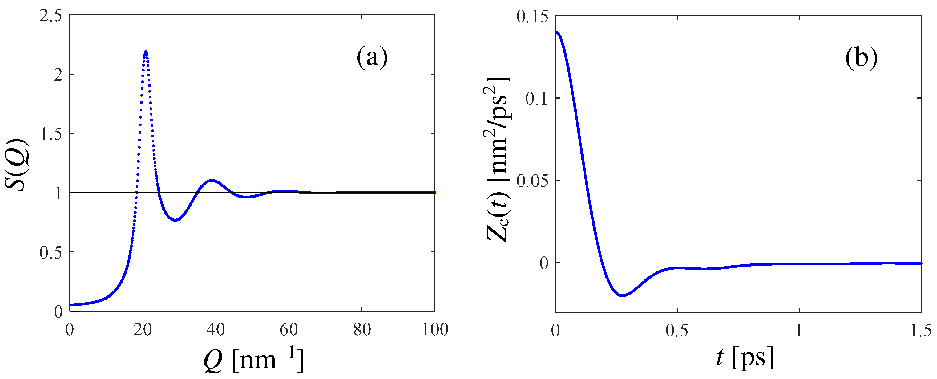
The results of the PI RPMD simulation of HD are reported in Figure 1, where both and the canonical VAF (see Appendix B) are displayed. The latter shows the expected behavior for a dense liquid, with a negative minimum witnessing the rattling motion of the tagged molecule within the temporary cage formed by its neighbors. In Appendix B, we show how an accurate estimate of the self diffusion coefficient D can be obtained from the simulated VAF, finding the value D = 3.2 for HD at the mentioned thermodynamic state. This is a significant outcome of this work, given the lack of literature values for D.
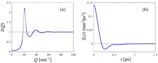
Figure 1.
(a): Static structure factor obtained from the PI RPMD calculation for HD at 17 K and n = 24.37 . (b): Simulated canonical VAF (see Appendix B) at the mentioned thermodynamic state of HD.
Specific calculations of the form factors of HD and of Equation (7) within the GA and Sköld approximations were performed by using the molecular parameters and neutron scattering lengths listed in Table A1 of Appendix A.
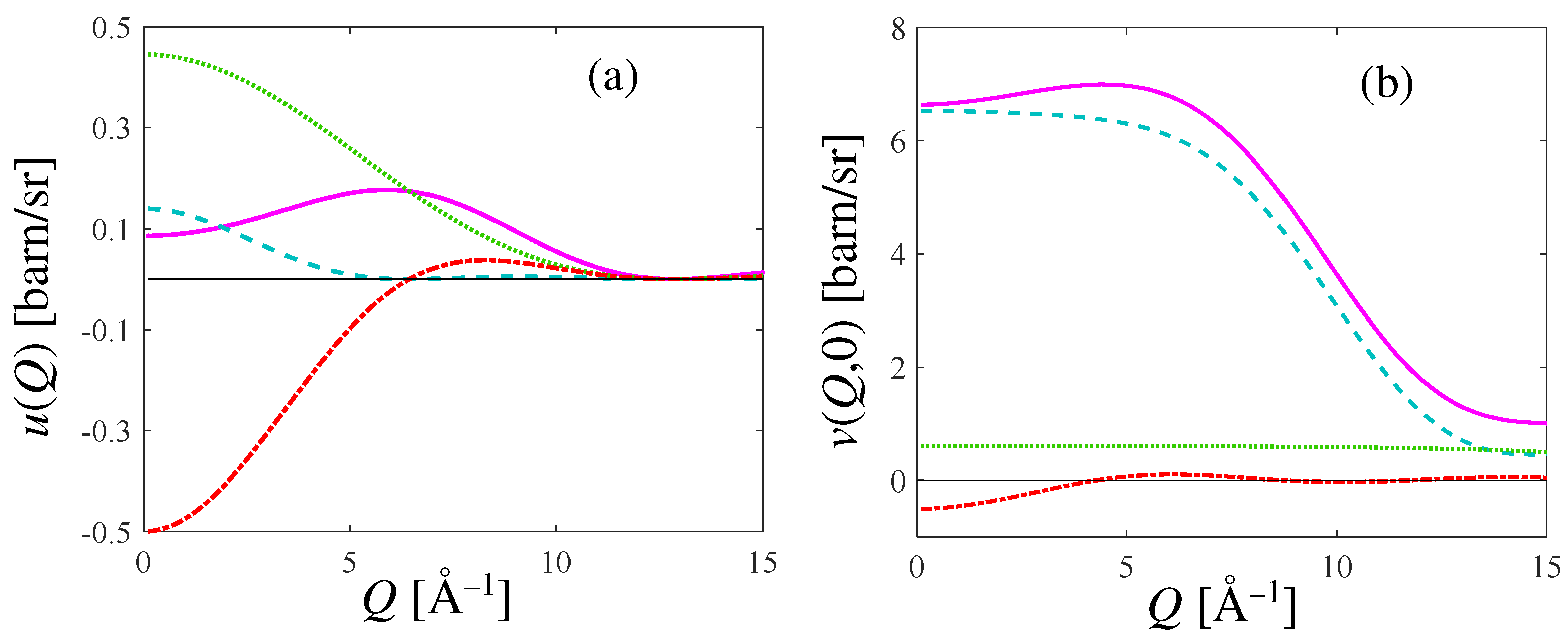
In Figure 2, we show the general features of the inter- and intramolecular form factors, and , as a function of the exchanged wavevector Q. The various terms contributing, respectively, to Equation (A17) and, at , to Equation (A12), are also displayed separately. Note that while does not depend on the incident energy, may vary with because, in practical implementations of the summation of Equation (A12), the number of rotovibrational transitions grows with incident energy. The example of Figure 2 refers, in particular, to an incident energy = 80 meV. As evident from Figure 2, the intramolecular form factor of HD overwhelms the intermolecular one, as expected.
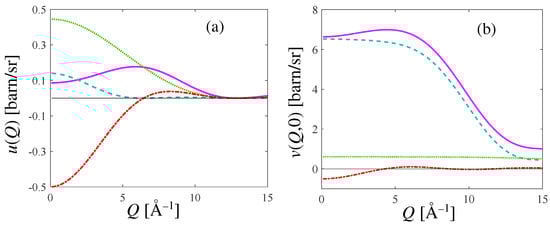
Figure 2.
(a): Intermolecular form factor (pink curve) according to Equation (A17) for HD at 17 K. (b): Intramolecular form factor (pink curve) from Equation (A12) calculated at and = 80 meV, for HD at the same temperature as in (a). In both panels, the three different terms of the quoted equations are also plotted: the contribution due to H is the dashed cyan curve, the one due to D is the green dotted curve, and the cross HD term is the red chain curve; their sum provides the pink curves.
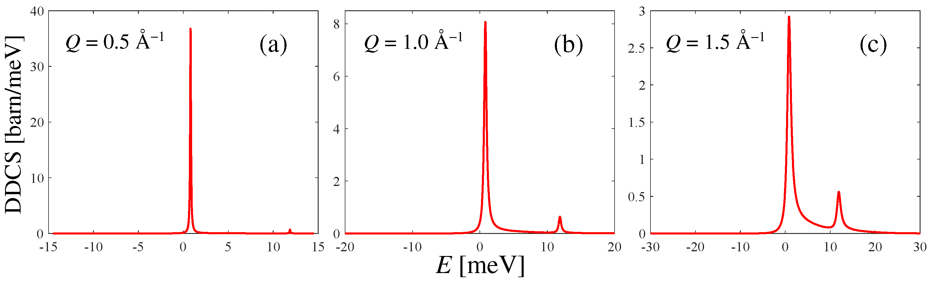
Examples of the DDCS spectra according to Equation (7) for = 80 meV are shown in Figure 3 at three selected Q values. The typical asymmetry of the spectra of quantum systems, as well as the rotational line at about 11 meV, can be better appreciated with a growing Q. Instead, due to the rather low temperature, the detailed balance strongly depletes the anti-Stokes line , which is present despite the low population (the level of HD at 17 K corresponds to a 0.16% occupation probability), but not appreciable on the scale of the figure. The example value chosen for allows to span a reasonable exchanged-energy range, and is a plausible choice if one were interested in performing a DDCS measurement on liquid HD, similarly to what was performed in Ref. [7] for liquid . Of course, as mentioned in Section 2, before comparison with any (forthcoming) experimental DDCS result, the spectra of Figure 3 should be convoluted with the energy resolution function of the used instrument.

Figure 3.
Calculated double differential cross section of HD at an incident neutron energy = 80 meV and at three example Q values, for 17 K. In panels (b,c), the rotational line at 11 meV starts to be appreciable compared to the elastic one. The progressive broadening and increasing detailed-balance asymmetry of the lines can also be observed as Q grows.
It is worth stating, finally, that the total DDCS of Figure 3, i.e., including the distinct dynamics, differs negligibly, at all Q values and at all incident energies, from its self component alone (not shown in the figure), as predictable from the very small values of of Figure 2. This simply means that HD is a “true” predominantly incoherent scatterer at all incident energies, even more than para-. Indeed, the absence of spin correlations in HD does not introduce different scattering cross sections according to the parity of the levels involved in the transitions and the spin statistics of the nuclei in the molecule. Conversely, in para-, if is insufficient to excite the first rotational line , then only the even–even transition contributes, and spin correlations can be found [19] to weight such kinds of transitions only by the coherent cross section. Therefore, at some incident energies ( meV), para- behaves coherently and the distinct dynamics plays a role. In HD, this is never the case, and the huge incoherent cross section of H dominates the scattering behavior independently of .
In order to make a comparison with the experimental total cross section possible, the DDCS of HD was calculated at K as a function of scattering angle and exchanged energy at various values of the incident energy ranging between 1 and 85 meV. At such energies, only rotations are excited and the main contribution to the spectra comes from the elastic line and the mentioned Stokes transition (when excited).
Double integration of the DDCS over the exchanged energy and solid angle, according to:
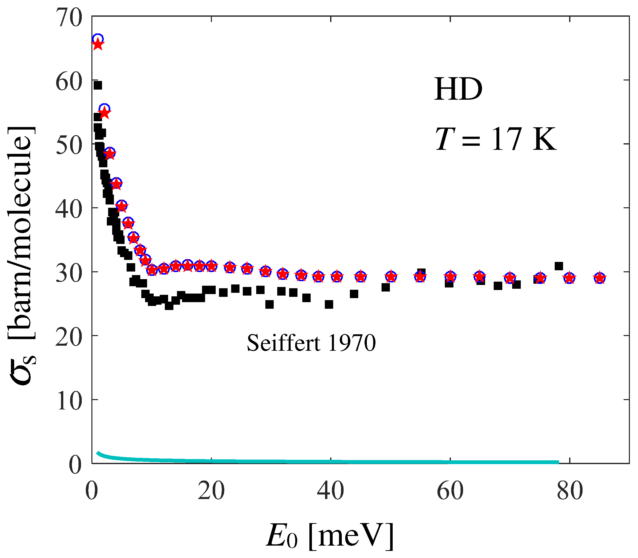
provides the total scattering cross section shown in Figure 4, in comparison with Seiffert’s data [21], from which the known absorption cross section [41] has been subtracted: in formulas, . The effect of the neglect of the distinct part in the calculation of is observed to be very small (compare the blue circles with the red stars in Figure 4), and slightly appreciable only at very low values.
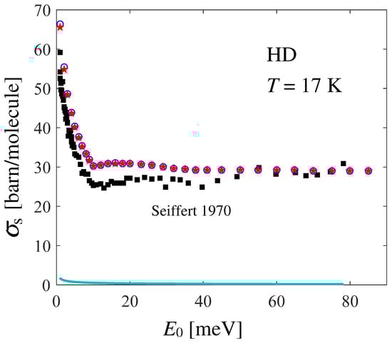
Figure 4.
Dependence on the incident energy of the total neutron scattering cross section of HD at 17 K, as obtained by absorption-subtracted Seiffert’s data [21] (black full squares) and by double integration of Equation (7) following Equation (9) (red stars), using the GA plus Sköld approximations for the CM translational dynamics. The blue empty circles represent the self component of alone, as obtained by double integration of the last term in Equation (7). The small effect of the absorption cross section of HD (cyan line) is also shown.
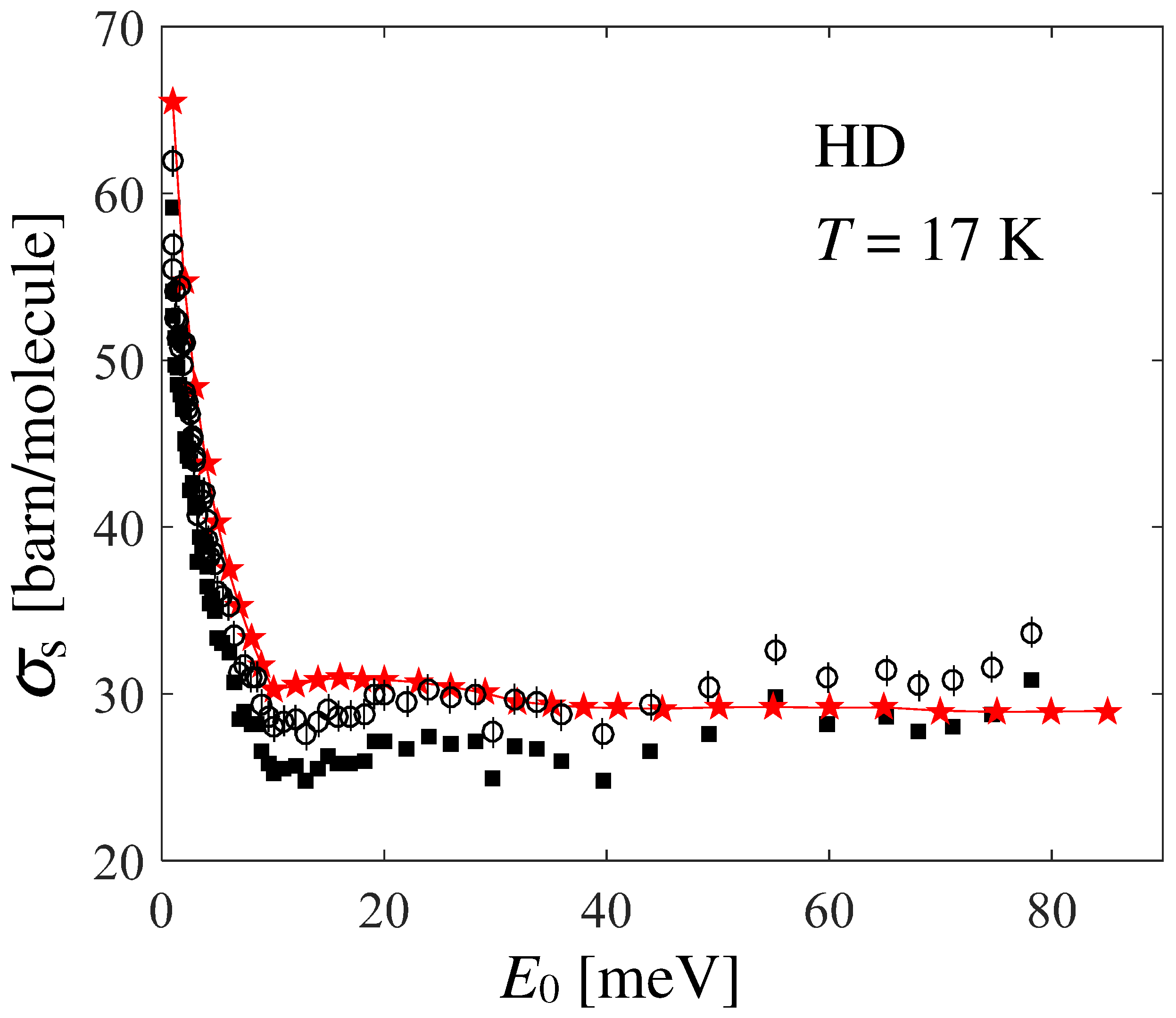
Unexpectedly, agreement between the data and calculations is not as good as the one found for normal and [4,20]. In Ref. [21], the author reports an average systematic error of and an average statistical error of for HD. Figure 5 shows the possible effect of shifting Seiffert’s data upwards by the systematic error (empty circles), while statistical uncertainties are taken into account by the corresponding error bars. By doing so, a good agreement is recovered at all energies (given that the experimental data points are rather scattered), except in the low-energy range meV, a disagreement which is worth investigating and discussing.
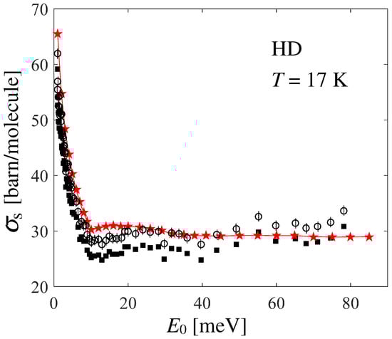
Figure 5.
Black full squares and red stars with thin line represent Seiffert’s data and present calculations, respectively, like in Figure 4. Empty circles with error bars take the systematic and statistical uncertainties of the measurements into account, as explained in the text.
4. Discussion
Trying to explore the reasons for the mismatch in the subthermal region, a possible effect of sample contamination might be considered. Information on this can be found in another paper by Seiffert [22], which reports the following composition determined by mass spectrometry: 94% HD, 5.5% and 0.5% . However, it is not specified whether the systematic error estimated by the author already included the role played by the impurities, or if these have to be considered as an additional source of error. Moreover, normal cannot be assumed to be part of the mixture, since even a small amount would provide total cross section values higher than those calculated for pure HD. This can be understood by considering the cross section monotonic behavior reported for n- in Refs. [20,21]. Conversely, the much lower cross section of para- in the range meV might well explain the discrepancy.
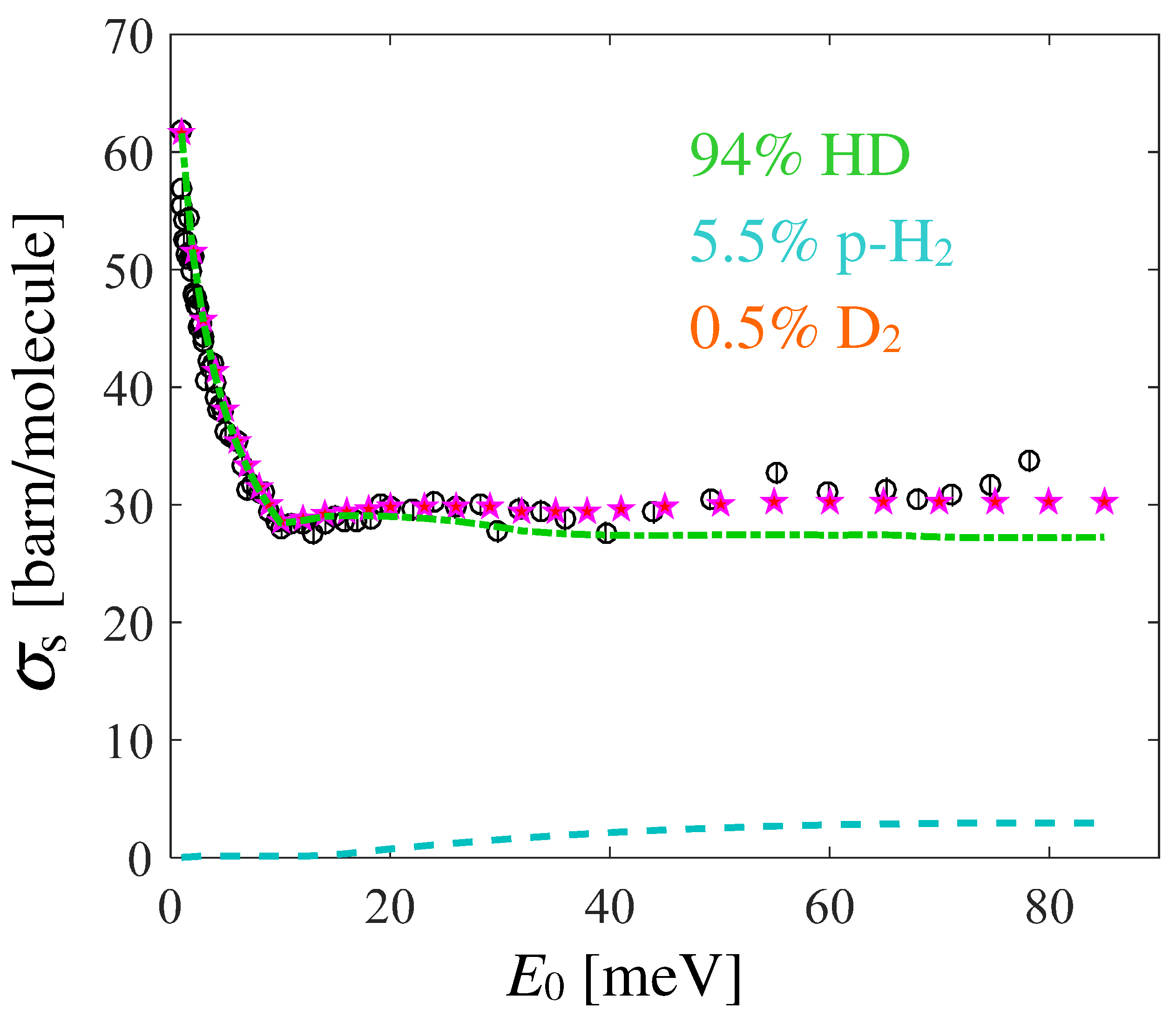
Preliminary calculations for the pure HD and the mentioned mixture were performed in past years using the Gaussian lineshape of the ideal gas for , finding an overall disagreement even by accounting for the presence of impurities [42], and which could not be recovered, even by adding the declared systematic errors. Here, however, we also adopted the more refined RPMD-based GA approach for HD, so it is worth analyzing the possible improvements due to the model lineshape. Although the available data for and para- are not exactly at 17 K, we combined the various calculations (all based on the GA and on quantum evaluations of the VAF) according to the declared composition, and report the results in Figure 6. The agreement is now very good at almost all energies. These results confirm both the sample contamination (likely not included in the estimate of systematic errors) but, more importantly, the improvements introduced by the use of quantum-compliant lineshapes, with respect to the earlier ideal gas modeling [42].
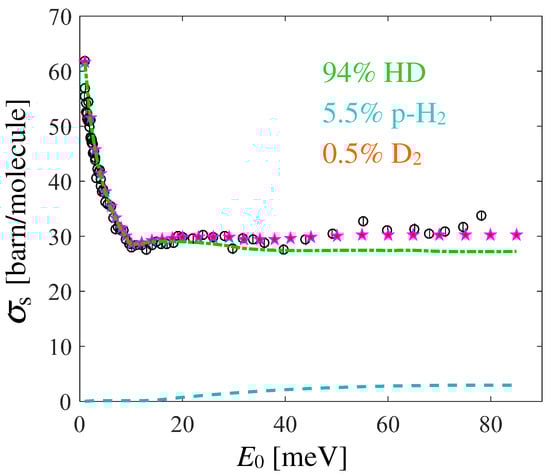
Figure 6.
Black empty circles with error bars are the experimental data corrected for the systematic errors, and pink stars are the GA-based calculations for the hydrogen isotopes mixture reported in the legend. The contribution of is not shown, since it is negligible on the scale of the figure, while the para- (dashed cyan curve) and HD (chain green curve) ones are also shown.
Nonetheless, the impressive result shown in Figure 6 has been obtained by assuming a well-defined direction of the systematic effects: an assumption the correctness of which we are, of course, not able to prove. A separate preliminary study [43], based on combining the earlier work of Ref. [14] with the approaches described in Ref. [6], indicated, on average, a roughly 10% lower cross section between 10 and 80 meV compared to the results presented here. Although the source of this discrepancy is under detailed investigation, it anyway emerges very clearly that new accurate measurements, as those performed in recent years for para-, are also highly auspicable for HD.
5. Conclusions
This work completes the picture of the calculation of the neutron double differential cross section of diatomic molecules, providing formulas for a heteronuclear vibrating rotor at low temperature. The interest for a treatment of the heteronuclear case, and particularly for hydrogen deuteride, was triggered by possible applications of this fluid in neutron moderation. Unfortunately, the lack of experimental DDCS data for HD prevents one from a stringent test of the calculations. It is, therefore, clear that our capability to predict the neutron DDCS of this cryogenic liquid and the setting up of reliable scattering libraries would profit from accurate inelastic scattering experiments and improved quantum simulation methods. Similar importance would have experimental work aimed at the determination of the thermodynamic properties of HD, at least in the low temperature dense liquid region useful in applications.
Author Contributions
Conceptualization, E.G.; methodology, U.B., E.G. and M.C.; software, E.G., U.B., D.D.D. and J.I.M.D.; formal analysis E.G. and D.D.D.; data curation, E.G., D.D.D. and J.I.M.D.; writing original draft preparation, E.G.; writing review and editing, all authors; funding acquisition, E.G. All authors have read and agreed to the published version of the manuscript.
Funding
This work has been funded by the Next Generation EU project PRIN-2022JWAF7Y.
Institutional Review Board Statement
Not applicable.
Informed Consent Statement
Not applicable.
Data Availability Statement
All data reported in this work are available on request.
Acknowledgments
The authors are grateful to Daniele Colognesi for fruitful discussions and a critical reading of the manuscript.
Conflicts of Interest
The authors declare no conflicts of interest. The funders had no role in the design of the study; in the collection, analyses, or interpretation of data; in the writing of the manuscript; or in the decision to publish the results.
Abbreviations
The following abbreviations are used in this manuscript:
| CM | center of mass |
| CMD | centroid molecular dynamics |
| DDCS | double differential scattering cross section |
| ESS | European spallation source |
| GA | Gaussian approximation |
| PI | path integral |
| RPMD | ring polymer molecular dynamics |
| VAF | velocity autocorrelation function |
Appendix A. Explicit Formulas for the Form Factors of Heteronuclear Diatomic Molecules
As reported in Equation (7) of Ref. [19], the form factors can be written as
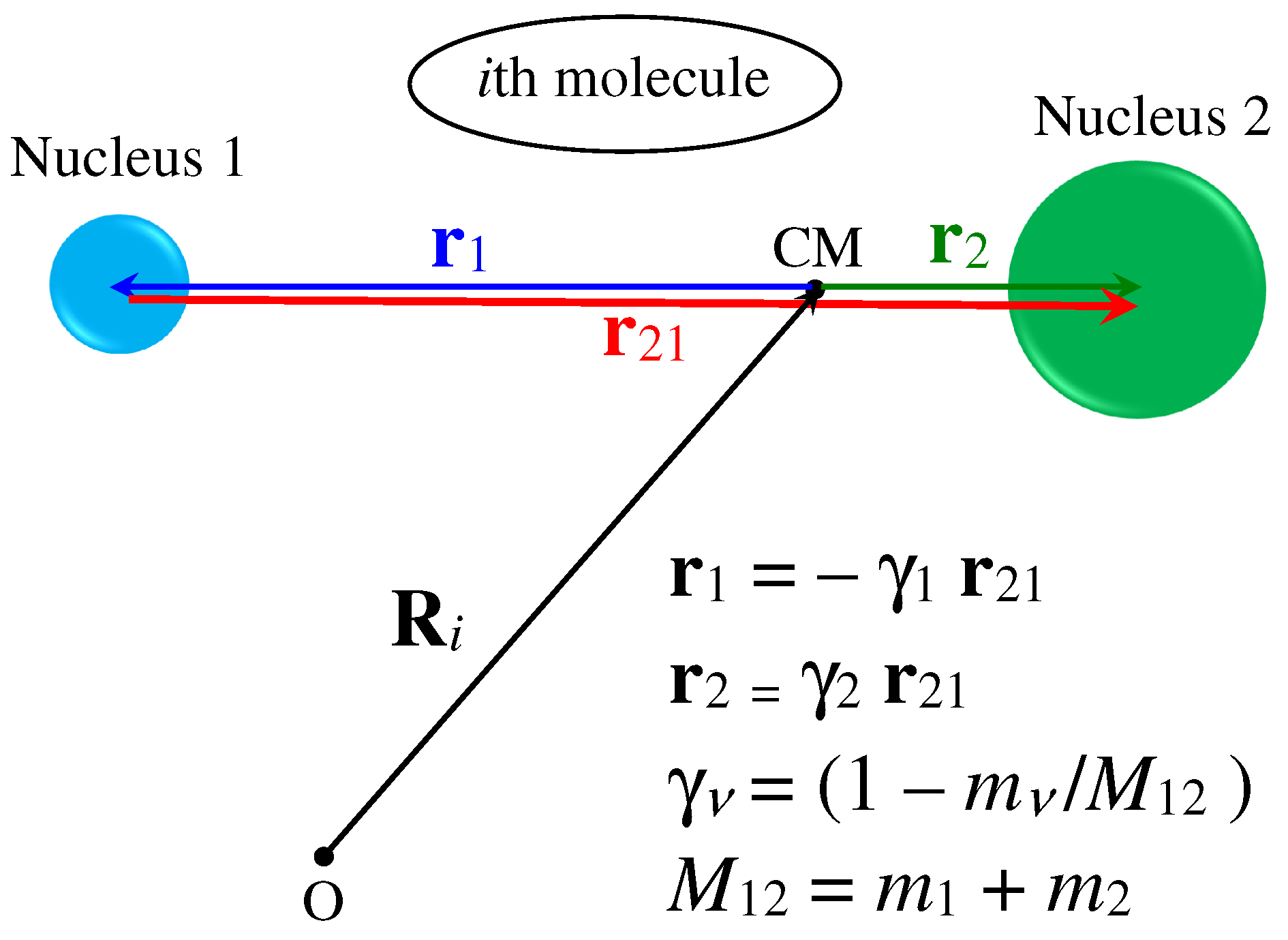
where and are the coherent and incoherent scattering lengths of the th nucleus in the molecule, which, in the most general case, is assumed to be characterized by a total of n (not necessarily different) nuclei. In the above equations, is the vector defining the position, at , of the th nucleus with respect to the CM of the molecule. Figure A1 summarizes the various definitions in the simple case we are interested in, i.e., with nucleus 1 (e.g., H) different from nucleus 2 (e.g., D).
The form factors are seen to involve the calculation of matrix elements of the kind , where denotes a generic rotovibrational state of the molecule. Subscripts 0 and 1 are used to indicate the initial (before scattering) and final (after scattering) molecular state, respectively. This, of course, can be written explicitly by adopting the usual notation for the rotational and vibrational quantum numbers, i.e., , with the last equality descending from the mentioned hypothesis of negligible coupling between rotations and (harmonic) vibrations.
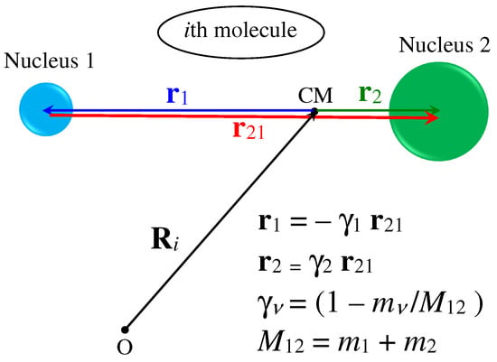
Figure A1.
Geometry and position vectors defined for the case of a heteronuclear diatomic molecule. The positions of the nuclei with respect to the CM are expressed by the appropriate fractions and of the internuclear distance vector (red arrow) joining the two nuclei of mass and , respectively. is the total molecular mass. Note that is meant to represent the instantaneous value of the internuclear distance, which can further be written as , with x the bond stretching and the average equilibrium distance.
Equations (A1) and (A2) include the statistical average over the initial state probabilities governed by the Boltzmann thermal distribution. Since the molecules are assumed to lie initially in the ground vibrational state (), it is possible to write . Finally, the time dependence in Equation (A2) comes simply from the Heisenberg representation of as , where is the total (rotational plus vibrational) Hamiltonian, ℏ is the reduced Planck constant, and we defined the transition frequency as . For a diatomic molecule, the latter can obviously also be written as , with the frequency of the harmonic oscillator of mass , i.e., corresponding to the reduced mass of the two-body system of total mass , and whose energy levels are given by .
The rotational energy levels of a free rotor are given by , with B being the rotational constant and D accounting for the centrifugal distortion.
The various parameters and scattering lengths specifically used for HD are given in Table A1.
Starting from Equations (A1) and (A2), one can explicitly write
where [13] results from the average of the scattering length over neutron and nuclear spin states which, in the uncorrelated case, can be performed separately from those involving position dependent operators.

Table A1.
Basic quantities used in the present calculations for HD.
Table A1.
Basic quantities used in the present calculations for HD.
| Parameter | Description |
|---|---|
| B = 5.538 meV [44] | Rotational constant in the vibrational ground state |
| D = 0.003263 meV [44] | Centrifugal distortion coefficient in the vibrational ground state |
| = 450.38 meV [44] | Quantum of vibrational energy |
| = 0.74142 Å [44] | Equilibrium internuclear distance |
| = 1.00794 a.m.u. | Mass of the proton |
| = 2.01410 a.m.u | Mass of the deuteron |
| Fraction of the internuclear distance pertaining to the H nucleus | |
| Fraction of the internuclear distance pertaining to the D nucleus | |
| = −3.7406 fm [41] | Coherent scattering length of the H nucleus |
| = 25.274 fm [41] | Incoherent scattering length of the H nucleus |
| = 6.674 fm [41] | Coherent scattering length of the D nucleus |
| = 4.033 fm [41] | Incoherent scattering length of the D nucleus |
By following Figure A1, and using the synthetic notation for , Equation (A4) becomes
where, in the last member, we introduced the internuclear vector , duly weighted, through the factor , by the mass of the nucleus under consideration. Note that in the adopted notation, both and are positive. Moreover, , while when .
All terms in Equation (A5) require the evaluation of the generic matrix element . In Equation (A5), the vibrational matrix element regarding, for instance, nucleus 2 (, with ), can be written as
where we explicitly wrote the scalar product posing , being the angle between Q and . Note that the prime is used here to distinguish the present angular coordinates from those related to the geometry of a scattering experiment used in the main text. In Equation (A6), the internuclear distance was also expressed as the sum of the equilibrium one, , and the bond stretching x. Finally, we defined . Care must be taken in the case of nucleus 1, where the change of the sign in the exponential at the first member of Equation (A6), when is replaced by , with , is transmitted to both exponentials of the last member of the equation.
In order to evaluate the last member of Equation (A6), we direct the reader to the quantum mechanical treatment of a one-dimensional harmonic oscillator [45] of mass , which provides in terms of the Bose creation and annihilation operators obeying the commutation relation . Using the properties (which is valid in the present case) and , the exponential of an operator, and considering the way operates on vibrational levels (leading, e.g., to ), it is possible to find that, for nucleus 2, we have
where we defined and . For nucleus 1, the vibrational matrix element is similar to Equation (A7), with replaced by .
The next step consists of the calculation of the rotational matrix element
where we introduced the spherical harmonics [45], omitting for brevity their argument , and integration is performed over the solid angle . Well-known properties (see, e.g., [46]) can be used to rewrite Equation (A8) in terms of appropriate Clebsch–Gordan coefficients, , and Legendre polynomials of order l, , with (see [42] for further details).
We can finally calculate the self-atomic terms in Equation (A5) according to
which is valid for any j. In analogy with Ref. [19], we can here define the integrals for nucleus 2 as
which will be used in what follows to shorten the notation. Note that the first exponential in the integrand is an even function of . So, if the complex exponential is split according to Euler formula, the former does not alter the well-defined parity of the remaining product function. Again, for nucleus 1, must be replaced by or, equivalently, we can define . Therefore, the distinct-atomic “cross” term turns out to be
Combining Equations (A5), (A9), (A10) and (A11), the intramolecular form factor of a heteronuclear diatomic fluid turns out to be
where
denotes the time-independent part of the intramolecular form factor.
It can be shown that Equation (A12) can also be written in a way that disentangles the roles played by and l, and is governed exclusively by the parity of l, i.e.,
where we recall that, by definition, .
As mentioned, the advantage of such a formulation for becomes evident in the homonuclear case, for which , , , , , and Equation (A14) can be cast in the elegant form
which is effectively identical to Equation (31) given in Ref. [19] for the uncorrelated spin case. We specified effectively because, for the ease of notation here, formal differences appear between the formulas in Ref. [19] and the present ones. In fact, the quantities (when ) and used here are not the same as in Ref. [19]. In particular, by renaming those defined in Ref. [19] as and (the subscript ho meaning “homonuclear”), we have
Nonetheless, Equations (A10) and (A15) only depend on the products and ; that is, exactly on and (since ).
The calculation of the intermolecular form factor given in Equation (A3) follows similar steps as before, but is further simplified by the fact that a quantum average of the exponential operators has to be performed, i.e., and in the previous formulas. In particular, we obtain
where was used to indicate . The final expression turns out to be
Note that the integrals are real-valued quantities in the case , . Therefore, in the homonuclear case, Equation (A17) actually adds up to
in agreement with Equation (27) of Ref. [19].
Appendix B. The Self Dynamic Structure Factor in the Gaussian Approximation
The dynamical information conveyed by the VAF is a keypoint in the development of models for the self part of the DDCS of viscous dense fluids. In the present case of a molecular liquid, the considered velocity autocorrelation is that of the molecular centers of mass
which is a complex-valued quantity satisfying and , with the latter property descending from the detailed balance principle.
However, the output of an RPMD simulation is the canonical (or Kubo-transformed [47]) VAF:
where H is the Hamiltonian operator of the system. The canonical VAF is a real and even function of time. By Fourier transformation of and , the respective frequency spectra and are obtained. Both functions are real and, while is even, can be decomposed into its symmetric and antisymmetric parts, , which are the Fourier transforms of Re and i Im , respectively. The three quantities just defined are all related to each other by the detailed balance requirement, , and the following relationships hold [26]:
The link between the above formalism about the VAF and the CM self intermediate scattering function is easily obtained by recalling that the latter is a Gaussian in wave vector Q in both the two limiting cases of hydrodynamic diffusion (, ) and the ideal gas behavior (, ) [25], with exactly known functions of time alone entering the expression of for a classical system:
where D is the self diffusion coefficient.
The Gaussian Approximation, introduced by Vineyard in 1958 [33], simply extends the above functionality to any intermediate time and Q value, i.e., it assumes that
This assumption was more deeply formalized, even for quantum systems, by Rahman and co-workers [34], who demonstrated that the self intermediate scattering function can be expressed as an infinite series of the form
whose first term, coinciding with Vineyard’s hypothesis, is related to the VAF spectrum. In particular, the final, and most significant expression of the GA in the Rahman et al. quantum picture provides the function of Equation (A24) as:
Such equations have been used in this work, starting from the RPMD simulation of , and developing the formalism previously described to implement the quantum GA in the DDCS algorithm.
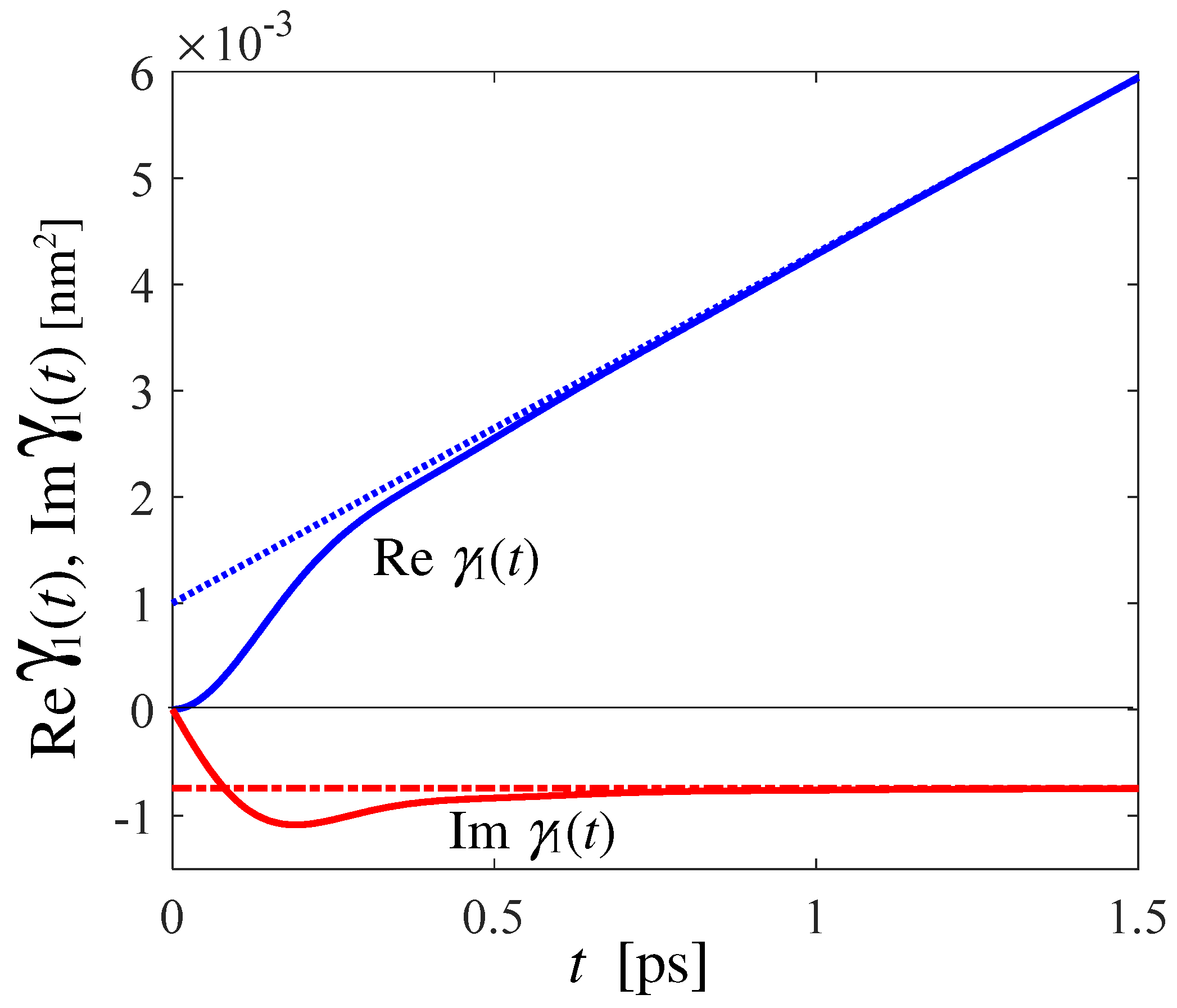
For the special case of HD at 17 K, from the canonical VAF of Figure 1b, we calculated Equation (A26) by obtaining the real and imaginary parts reported in Figure A2. Asimptotically, Re , which is proportional to the mean square displacement [34], tends to linear behavior with a slope that corresponds to the self diffusion coefficient D, while Im tends to a constant value, also related to D [34]. The asymptotic trends are shown in Figure A2 with dotted and dot-dashed lines. In particular, the slope of Re provides a self diffusion coefficient equal to D = 3.2 for HD, which is compatible with that of at a higher temperature (20.7 K), but a greater density (25.40 ) [4], which was = 3.8 .
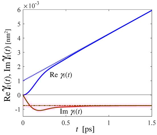
Figure A2.
Real (blue solid curve) and imaginary (red solid curve) parts of Equation (A26). The asymptotic trends are shown, respectively, as dotted blue and dot-dashed red lines.
Figure A2.
Real (blue solid curve) and imaginary (red solid curve) parts of Equation (A26). The asymptotic trends are shown, respectively, as dotted blue and dot-dashed red lines.
References
- Willis, B.T.M.; Carlile, C.J. Experimental Neutron Scattering; Oxford University Press: New York, NY, USA, 2009. [Google Scholar]
- Grammer, K.B.; Alarcon, R.; Barrón-Palos, L.; Blyth, D.; Bowman, J.D.; Calarco, J.; Crawford, C.; Craycraft, K.; Evans, D.; Fomin, N.; et al. Measurement of the scattering cross section of slow neutrons on liquid parahydrogen from neutron transmission. Phys. Rev. B 2015, 91, 180301. [Google Scholar] [CrossRef]
- Guarini, E.; Neumann, M.; Bafile, U.; Celli, M.; Colognesi, D.; Farhi, E.; Calzavara, Y. Velocity autocorrelation in liquid parahydrogen by quantum simulations for direct parameter-free computations of neutron cross sections. Phys. Rev. B 2015, 92, 104303. [Google Scholar] [CrossRef]
- Guarini, E.; Neumann, M.; Bafile, U.; Celli, M.; Colognesi, D.; Bellissima, S.; Farhi, E.; Calzavara, Y. Velocity autocorrelation by quantum simulations for direct parameter-free computations of the neutron cross sections. II. Liquid deuterium. Phys. Rev. B 2016, 93, 224302. [Google Scholar] [CrossRef]
- Marquez Damian, J.I.; DiJulio, D.D.; Muhrer, G. Nuclear data development at the European Spallation Source. arXiv 2021, arXiv:2103.06133v1. [Google Scholar] [CrossRef]
- DiJulio, D.D.; Marquez Damian, J.I.; Muhrer, G. Generation of thermal neutron scattering libraries for liquid para-hydrogen and ortho-deuterium using ring-polymer molecular dynamics. EPJ Web Conf. 2023, 284, 17006. [Google Scholar] [CrossRef]
- Guarini, E.; Barocchi, F.; Francesco, A.D.; Formisano, F.; Laloni, A.; Bafile, U.; Celli, M.; Colognesi, D.; Magli, R.; Cunsolo, A.; et al. Collective dynamics of liquid deuterium: Neutron scattering and approximate quantum simulation methods. Phys. Rev. B 2021, 104, 174204. [Google Scholar] [CrossRef]
- Butterworth, I.; Egelstaff, P.A.; London, H.; Webb, F.J. The production of intense cold neutron beams. Phil. Mag. 1957, 2, 917. [Google Scholar] [CrossRef]
- Sasaki, K.; Konno, M.; Hiraga, F.; Iwasa, H.; Kamiyama, T.; Kiyanagi, Y.; Iverson, E.B.; Carpenter, J.M. Experimental Studies on Neutronics of CH3D and HD Cold Neutron Moderators. In Proceedings of the JAERI-Conf 2001-002 and KEK Proceedings 2000-22, International Collaboration on Advanced Neutron Sources ICANS-XV, Tsukuba, Japan, 6–9 November 2000; Available online: https://inis.iaea.org/collection/NCLCollectionStore/_Public/33/010/33010071.pdf?r=1 (accessed on 18 March 2024).
- Ageron, P. Special Neutron Sources. In Proceedings of the Conference Organized by the International Atomic Energy Agency in Collaboration with the Jülich Nuclear Research Centre. Neutron Scattering in the ‘Nineties, Jülich, Germany, 14–18 January 1985; Available online: https://inis.iaea.org/collection/NCLCollectionStore/_Public/16/076/16076003.pdf (accessed on 18 March 2024).
- Gobrecht, K.; Gutsmiedl, E.; Scheuer, A. Status report on the cold neutron source of the Garching neutron research facility FRM-II. Physica B 2002, 311, 148. [Google Scholar] [CrossRef]
- Young, J.A.; Koppel, J.U. Slow neutron scattering by molecular hydrogen and deuterium. Phys. Rev. A 1964, 135, 603. [Google Scholar] [CrossRef]
- Sears, V.F. Theory of cold neutron scattering by homonuclear diatomic liquids. I Free rotation. Can. J. Phys. 1966, 44, 1279. [Google Scholar] [CrossRef]
- Lurie, N.A. Influence of rotational levels on slow-neutron scattering by linear gases. J. Chem. Phys. 1967, 46, 352. [Google Scholar] [CrossRef]
- Colognesi, D.; Formisano, F.; Ramirez-Cuesta, A.J.; Ulivi, L. Lattice dynamics and molecular rotations in solid hydrogen deuteride: Inelastic neutron scattering study. Phys. Rev. B 2009, 79, 144307. [Google Scholar] [CrossRef]
- Xu, M.; Ulivi, L.; Celli, M.; Colognesi, D.; Bačić, Z. Rigorous quantum treatment of inelastic neutron scattering spectra of a heteronuclear diatomic molecule in a nanocavity: HD in the small cage of structure II clathrate hydrate. Chem. Phys. Lett. 2013, 563, 1. [Google Scholar] [CrossRef]
- Colognesi, D.; Powers, A.; Celli, M.; Xu, M.; Bačić, Z.; Ulivi, L. The HD molecule in small and medium cages of clathrate hydrates: Quantum dynamics studied by neutron scattering measurements and computation. J. Chem. Phys. 2014, 141, 134501. [Google Scholar] [CrossRef] [PubMed]
- Zoppi, M. Neutron scattering of homonuclear diatomic liquids. The rotating harmonic oscillator model. Physica B 1993, 183, 235. [Google Scholar] [CrossRef]
- Guarini, E. The neutron double differential cross-section of simple molecular fluids: Refined computing models and nowadays applications. J. Phys. Condens. Matter 2003, 15, R775. [Google Scholar] [CrossRef]
- Guarini, E. The neutron cross section of the hydrogen liquids: Substantial improvements and perspectives. arXiv 2014, arXiv:2104.05004. [Google Scholar]
- Seiffert, W.D. Messung der Streuquerschnitte von Flüssigem und Festem Wasserstoff, Deuterium und Deuteriumhydrid für Thermische Neutronen, Euratom Report No. EUR 4455d. 1970; unpublished.
- Seiffert, W.D.; Weckermann, B.; Misenta, R. Messung der Streuquerschnitte von flüssigem und festem Wasserstoff, Deuterium und Deuteriumhydrid für thermische Neutronen. Z. Naturforsch. A 1970, 25, 967. [Google Scholar] [CrossRef]
- van Kranendonk, J. Solid Hydrogen; Plenum: New York, NY, USA, 1983. [Google Scholar]
- Ashcroft, N.W.; Mermin, N.D. Solid State Physics; Saunders College: Philadelphia, PA, USA, 1976. [Google Scholar]
- Hansen, J.P.; McDonald, I.R. Theory of Simple Liquids, 2nd ed.; Academic Press: London, UK, 1986. [Google Scholar]
- Bellissima, S.; Neumann, M.; Bafile, U.; Colognesi, D.; Barocchi, F.; Guarini, E. Density and time scaling effects on the velocity autocorrelation function of quantum and classical dense fluid parahydrogen. J. Chem. Phys. 2019, 150, 074502. [Google Scholar] [CrossRef]
- Cao, J.; Voth, G.A. The formulation of quantum statistical mechanics based on the Feynman path centroid density. II. Dynamical properties. J. Chem. Phys. 1994, 100, 5106. [Google Scholar] [CrossRef]
- Jang, S.; Voth, G.A. Path integral centroid variables and the formulation of their exact real time dynamics. J. Chem. Phys. 1999, 111, 2357. [Google Scholar] [CrossRef]
- Hone, T.D.; Voth, G.A. A centroid molecular dynamics study of liquid para-hydrogen and ortho-deuterium. J. Chem. Phys. 2004, 121, 6412. [Google Scholar] [CrossRef] [PubMed]
- Craig, I.R.; Manolopoulos, D.E. Quantum statistics and classical mechanics: Real time correlation functions from ring polymer molecular dynamics. J. Chem. Phys. 2004, 121, 3368. [Google Scholar] [CrossRef]
- Miller, T.F., III; Manolopoulos, D.E. Quantum diffusion in liquid para-hydrogen from ring-polymer molecular dynamics. J. Chem. Phys. 2005, 122, 184503. [Google Scholar] [CrossRef] [PubMed]
- Habershon, S.; Manolopoulos, D.E.; Markland, T.E.; Miller, T.F., III. Ring-Polymer Molecular Dynamics: Quantum effects in chemical dynamics from classical trajectories in an extended phase space. Annu. Rev. Phys. Chem. 2013, 64, 387. [Google Scholar] [CrossRef] [PubMed]
- Vineyard, G.H. Scattering of Slow Neutrons by a Liquid. Phys. Rev. 1958, 110, 999. [Google Scholar] [CrossRef]
- Rahman, A.; Singwi, K.S.; Sjölander, A. Theory of slow neutron scattering by liquids. I. Phys. Rev. 1962, 126, 986. [Google Scholar] [CrossRef]
- Sköld, K. Small energy transfer scattering of cold neutrons from liquid argon. Phys. Rev. Lett. 1967, 19, 1023. [Google Scholar] [CrossRef]
- Roder, H.M.; Childs, G.E.; McCarty, R.D.; Angerhofer, P.E. Survey of the Properties of the Hydrogen Isotopes below Their Critical Temperatures; NBS Technical Note 641; National Bureau of Standards: Gaithersburg, MD, USA, 1973. [Google Scholar]
- Kapil, V.; Rossi, M.; Marsalek, O.; Petraglia, R.; Litman, Y.; Spura, T.; Cheng, B.; Cuzzocrea, A.; Meißner, R.H.; Wilkins, D.M.; et al. i-PI: A universal force engine for advanced molecular simulations. Comput. Phys. Comm. 2019, 236, 214. [Google Scholar] [CrossRef]
- Silvera, I.F.; Goldman, V.V. The isotropic intermolecular potential for H2 and D2 in the solid and gas phases. J. Chem. Phys. 1978, 69, 4209. [Google Scholar] [CrossRef]
- Brehm, M.; Kirchner, B. TRAVIS—A Free Analyzer and Visualizer for Monte Carlo and Molecular Dynamics Trajectories. J. Chem. Inf. Model. 2011, 51, 8. [Google Scholar] [CrossRef]
- Brehm, M.; Kirchner, B. TRAVIS—A free analyzer for trajectories from molecular simulation. J. Chem. Phys. 2020, 152, 164105. [Google Scholar] [CrossRef] [PubMed]
- Sears, V.F. Neutron scattering lengths and cross sections. Neutron News. 1992, 3, 26. [Google Scholar] [CrossRef]
- Guarini, E. The neutron cross section of low-temperature heteronuclear diatomic fluids. arXiv 2021, arXiv:2107.05422. [Google Scholar]
- Huusko, A. Calculation of Neutron Scattering Libraries for Liquid Ortho-Deuterium and Hydrogen Deuteride. Master’s Thesis, Lund University, Lund, Sweden, 2021. Available online: https://lup.lub.lu.se/search/ (accessed on 18 March 2024).
- Huber, K.P.; Herzberg, G. Molecular Spectra and Molecular Structure IV. Constants of Diatomic Molecules; van Nostrand-Reinhold: New York, NY, USA, 1979. [Google Scholar]
- Messiah, A. Quantum Mechanics, 11th ed.; North-Holland: Amsterdam, The Netherlands, 1986; Volumes 1 and 2. [Google Scholar]
- Gray, C.G.; Gubbins, K.E. Theory of Molecular Fluids; Clarendon: Oxford, UK, 1984. [Google Scholar]
- Kubo, R. The fluctuation-dissipation theorem. Rep. Prog. Phys. 1966, 29, 255. [Google Scholar] [CrossRef]
Disclaimer/Publisher’s Note: The statements, opinions and data contained in all publications are solely those of the individual author(s) and contributor(s) and not of MDPI and/or the editor(s). MDPI and/or the editor(s) disclaim responsibility for any injury to people or property resulting from any ideas, methods, instructions or products referred to in the content. |
© 2024 by the authors. Licensee MDPI, Basel, Switzerland. This article is an open access article distributed under the terms and conditions of the Creative Commons Attribution (CC BY) license (https://creativecommons.org/licenses/by/4.0/).