Abstract
This study introduces a compact Raman spectrometer with a 1064 nm excitation laser coupled with a fiber probe and an inexpensive motorized stage, offering a promising alternative to widely used Raman imaging instruments with 785 nm excitation lasers. The benefits of 1064 nm excitation for biomedical applications include further suppression of fluorescence background and deeper tissue penetration. The performance of the 1064 nm instrument in detecting cancer in human bladder resectates is demonstrated. Raman images with 1064 nm excitation were collected ex vivo from 10 human tumor and non-tumor bladder specimens, and the results are compared to previously published Raman images with 785 nm excitation. K-Means cluster (KMC) analysis is used after pre-processing to identify Raman signatures of control, tumor, necrosis, and lipid-rich tissues. Hierarchical cluster analysis (HCA) groups the KMC centroids of all specimens as input. The tools for data processing and hyperspectral analysis were compiled in an open-source Python library called SpectraMap (SpMap). In spite of lower spectral resolution, the 1064 nm Raman instrument can differentiate between tumor and non-tumor bladder tissues in a similar way to 785 nm Raman spectroscopy. These findings hold promise for future clinical hyperspectral Raman imaging, in particular for specimens with intense fluorescence background, e.g., kidney stones that are discussed as another widespread urological application.
1. Introduction
Optical and spectral technologies offer many opportunities in intraoperative histopathology [1]. Among the techniques that are already approved or close to being applied in standard clinical practice for in vivo and ex vivo monitoring are Raman-based methods [2]. Raman spectroscopy probes inherent molecular vibrations without markers by inelastic scattering of monochromatic laser light. The general advantages are no or minimal sample preparation, no need for extrinsic markers, and high specificity of the spectrum of Raman-active vibrations. The main limitation of spontaneous Raman spectroscopy as a biomedical tool is due to the weak scattering cross-sections of biomolecules and the fluorescence emission of chromophores that overlap or obscure the Raman signals even in trace amounts. Several Raman variants were developed in the past decade to overcome this limitation, including (i) coherent Raman scattering [3,4], (ii) time-gated Raman scattering [5], and (iii) shifted excitation Raman difference spectroscopy [6,7] that are all experimentally complex, (iv) surface-enhanced Raman scattering [8,9] which requires complex preparation protocols involving nanostructured surfaces or particles, and (v) data processing procedures [10,11] that require expert knowledge in data science. An alternative approach that was developed more than two decades ago is spontaneous Raman spectroscopy with 1064 nm laser excitation. As this excitation wavelength is not absorbed by most chromophores, the acquired Raman spectra are minimally affected by the fluorescence background. The first technical realization used the Fourier transformation (FT) principle with a liquid nitrogen-cooled germanium-based detector for the registration of Raman spectra [12]. With the advent of dispersive spectrometers with holographic transmissive gratings and indium gallium arsenide (InGaAs) based array detectors, a new generation of versatile Raman instruments was developed that are compact, less expensive, and more sensitive than FT–Raman systems [13,14]. In this work, a laser and spectrometer for 1064 nm Raman spectroscopy are coupled with a fiber-optic Raman probe, an inexpensive motorized stage, and a digital camera. As a first biomedical application, Raman images are collected from bladder tissue specimens for tumor identification.
Bladder cancer is the 10th most frequently diagnosed cancer worldwide (source: World Cancer Research Fund International [15]). Cystoscopy is the standard diagnostic method followed by excision of surgical biopsies and pathological inspection [16]. Raman spectroscopic-based techniques have been suggested as a complementary diagnostic tool to assess bladder tissues ex vivo in thin sections or biopsies and in vivo during cystoscopy. Raman papers in the context of bladder cancer between 2005 and 2022 have recently been summarized [17]. Of particular relevance for the current work was the characterization of bladder tissue using probe-based Raman spectroscopy [18]. As most Raman spectra in this study were affected by an intense background, a data processing workflow was presented to suppress the background. Subsequently, machine learning models distinguished tumor from non-tumor with sensitivity and specificity of 92% and 93%, respectively, and low-grade from high-grade tumor tissues with sensitivity and specificity of 85% and 83%, respectively. More recent work demonstrated the combination of a 2D spectrogram along with a convolutional neural network for the diagnosis of bladder cancer with an even higher accuracy of 99.2% [19]. Here, upscaling techniques were used to transform 1D Raman spectral data into a variety of 2D spectrograms. In addition, a weighted feature fusion network was constructed which was employed to evaluate multiple spectrograms. A translational approach introduced the combined use of in vivo Raman spectroscopy and in vivo cryoablation to detect and remove the residual bladder tumor during transurethral resection of bladder tumor (TURBT) [20]. First, reference Raman spectra were collected from a group of 74 bladder cancer patients, and a machine learning model was trained for classification. Then, an independent group of 26 patients accepted traditional TURBT, whereas another group of 27 patients accepted TURBT, followed by Raman scanning and cryoablation if Raman detected the existence of residual tumor. Interestingly, 2 in 27 patients had cancer recurrence in the Raman–Cryoablation group, while 8 in 26 patients had cancer recurrence in the traditional TURBT group during follow-up. This shows how the combined use of Raman and cryoablation can serve as adjuvant therapy to improve therapeutic effects and reduce recurrence rates.
The current work applies for the first time an in-house developed dispersive 1064 nm Raman instrument to collect Raman images from bladder tissue. The reduced background is expected to simplify the data processing and to contribute to improved tumor identification. The sample cohort consists of non-tumor and tumor specimens that were prepared from ten human bladder resectates. The samples were already studied by 785 nm Raman microscopic imaging [17] and the previous results are compared with the new results. As most bladder specimens showed an unusually low background in the 785 nm Raman study, the Raman analysis of four kidney stones were included in the discussion section. Two of them did not give usable Raman spectra at 785 nm excitation, whereas high quality spectra were acquired with the 1064 nm Raman system.
2. Materials and Methods
2.1. Dispersive Raman Instrument with 1064 nm Excitation Laser
A schematic of the dispersive Raman instrument with a 1064 nm excitation laser is depicted in Figure 1A. The compact spectrometer (Wasatch Photonics, Logan, UT, USA) offered a spectral range of 250–1850 cm−1 using a holographic transmissive grating. The spectral resolution was 10 cm−1 at a slit size of 50 µm. The spectrometer featured a 512-pixel InGaAs array detector (Hamamatsu G9214-512S, Hamamatsu, Japan, pixel size 25 × 500 nm), which was thermoelectrically cooled to −15 °C. A 1064 nm laser with a linewidth < 0.1 nm corresponding to <0.9 cm−1 (Innovative Photonics Solution, Plainsboro Township, NJ, USA) was coupled via a 105 µm multimode fiber to a Raman probe with a focusing lens of numerical aperture 0.3, offering a working distance of 12 mm (Wasatch Photonics, Logan, UT, USA). The Raman probe focused the laser to a spot diameter of roughly 200 µm. A collection fiber with a 600 µm core diameter guided the Raman scattered signal to the spectrometer. Raman images were acquired using an inexpensive three-dimensional stage (SainSmart Genmitsu CNC 3018-PRO, Shanghai, China). A USB-coupled full HD digital microscope camera (Facamword, Chicago, IL, USA) was installed next to the fiber probe, and the offset between the microscope and Raman probe was calibrated to define the region of interest. In-house LabVIEW (National Instruments, Austin, TX, USA) routines were developed to control the components and spectra acquisition. Raman images were acquired from bladder tissue samples with an exposure time of 10 s, laser power of 450 mW, and 400 to 500 µm step size.
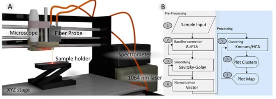
Figure 1.
Dispersive Raman instrument with 1064 excitation laser (A) with fiber probe, microscope, and motorized stage, and (B) hyperspectral processing algorithm provided by SpMap.
2.2. Data Analysis
The Python package SpMap performed all spectral processing [21]. The data processing workflow is shown in Figure 1B. SpMap provides several pre-processing tools, such as dark noise subtraction, wavelength and intensity calibration, cosmic ray correction, and filtering of spectra below an intensity threshold. To suppress detector and probe background noise, a dark spectrum (laser off) and probe background (laser on) without samples were collected. Then, the fingerprint region from 500 to 1800 cm−1 was selected. An advanced airPLS baseline correction [22] was applied to remove the remaining tissue and microscope system backgrounds. Finally, all spectra were smoothed with a Savitzky-Golay filter [23] and vector normalized.
After preprocessing, the first step involved the use of k-means cluster analysis (KMC) in the spectral range 600–1800 cm−1 to identify the main spectral signatures in each sample, such as control, tumor, necrosis, and lipid-rich tissues. KMC was also employed to reduce the size of data to a few clusters and increase the signal-to-noise ratios because each cluster centroid represents the mean of the cluster. These cluster centroids were then labeled based on the sample origin, i.e., whether they originated from a non-tumor or a tumor specimen. Hierarchical cluster analysis (HCA) was then performed in the spectral range 800–1150 cm−1 to arrange the KMC centroids found in the bladder tissue into the four categories, thereby reducing the computational cost. As the distance matrix in HCA can become large and calculation of the dendrogram can become time-consuming for large data sets, similar strategies have been applied before [24].
2.3. Study Population
The study used both non-tumor and tumor samples from ten human bladder resections obtained from the tissue bank of the Comprehensive Cancer Centre Freiburg (Freiburg im Breisgau, Germany). The samples were shipped on dry ice to Jena and stored at −80 °C until 785 nm Raman experiments. After finishing the 785 nm data collection, the samples were stored again in the −80 °C freezer until the 1064 nm Raman experiments. The size of each sample was approximately 10 × 10 mm2, and measurements were performed in a closed sample chamber without any sample preparation as described previously [17].
3. Results
3.1. K-Means Cluster Analysis of Tumor 3 and Control 5 Specimens
Figure 2 shows photomicrographs and KMC membership maps of control bladder sample 5 (Figure 2A,B) and tumor bladder sample 3 (Figure 2C,D). The spectral results followed the processing workflow shown in Figure 1B. Lipid-rich tissue can be found both inside and around the tissue sample (Figure 2B). Control tissue is most abundant in control specimen 5 (Figure 2B), and tumor tissue is most abundant throughout tumor specimen 3 (Figure 2D). Figure 2E–G shows cluster centroid spectra in the fingerprint region (600–1800 cm−1) of the control bladder, bladder tumor, and lipid-rich tissue, respectively. The tumor and control signatures show bands at 1003/1004, 1250–1308, and 1653/1661 cm−1, which are characteristic of phenylalanine, amide III, and amide I vibrations, respectively. Further bands at 858/859 and 930/939 cm−1 are assigned to collagen triple helices of fibrous proteins that are more intense in control than in tumor bladder. Besides the depleted collagen contributions, the band at 1076 cm−1 shifts toward 1091 cm−1, which points to elevated DNA contributions in tumor tissue. The bands around 1655 cm−1 are broader for control and tumor bladder than for lipids because the amide I band, which is a marker for protein secondary structures, has a larger width than the C=C band of lipids. Spectra of lipid-rich tissue has strong signatures at 1077 cm−1 for C–C vibrations, at 1304 and 1446 cm−1, which are characteristic of CH2 bending vibrations, and at 1269 and 1663 cm−1, that are characteristic of C=CH and C=C vibrations, respectively, in unsaturated lipids. Further spectral contributions in lipid-rich tissues are due to phosphate groups at 1077 cm−1 and C=O groups at 1746 cm−1, typical for phospholipids.
The 785 nm excited Raman spectra from the same specimens are included in Figure 2E–G for comparison [17]. The overall signature and band positions agree well. The main deviation near 1660 cm−1 is observed for the tumor (Figure 2F), which is tentatively assigned to lower spectral contributions of water near 1640 cm−1 in the 1064 nm Raman spectrum. Other deviations are related to the lower spectral resolution of the 1064 nm instrument than the 785 nm instrument. The resolution of the 1064 nm data is further affected by Savitzy–Golay smoothing, as indicated in Figure 1B. The lower resolution broadens the bands, which is particularly evident for the phenylalanine band at 1004 cm−1. Careful inspection of 785 nm Raman spectra resolves more bands of aromatic amino acids at 621, 643, 756, 1031, 1209, 1548, 1584, 1606, and 1620 cm−1 (see also Table S1 in the Supplementary Materials and spectra in the main text of Krafft et al. [17]). Another fine structure is better resolved in 785 nm Raman spectra of lipids at 1065 (C–C vibration), 1082 (phosphate vibration), and 1122 (C–C vibration) cm−1, which gives a broad envelope at 1077 cm−1 in 1064 nm Raman spectra. Such band overlap can be resolved by calculating the second derivative of spectra. A previous Raman study of cell classification using spectra of spectral resolution between 8 and 48 cm−1 demonstrated that the spectral information is not lost but conserved in lower-resolution spectra [25]. Consistent with similar cell classification for low- and high-resolution spectra in [25,26], tissue types could be distinguished by 1064 nm and 785 nm Raman spectroscopy at lower and higher spectral resolution, respectively.
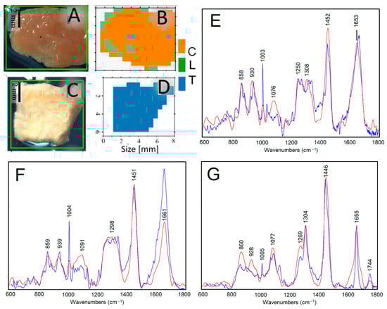
Figure 2.
K-means cluster analysis of Raman images: photomicrographs and cluster membership maps of control bladder sample 5 (A,B) and tumor bladder sample 3 (C,D), and cluster centroid spectra of control—C (E), tumor—T (F), and lipid-rich—L (G) tissues. Labels refer to 1064 nm Raman spectra (red traces) that are overlaid with 785 nm Raman spectra (blue traces) from the same specimens for comparison.
3.2. Overview of the Clustering Results of the Specimens
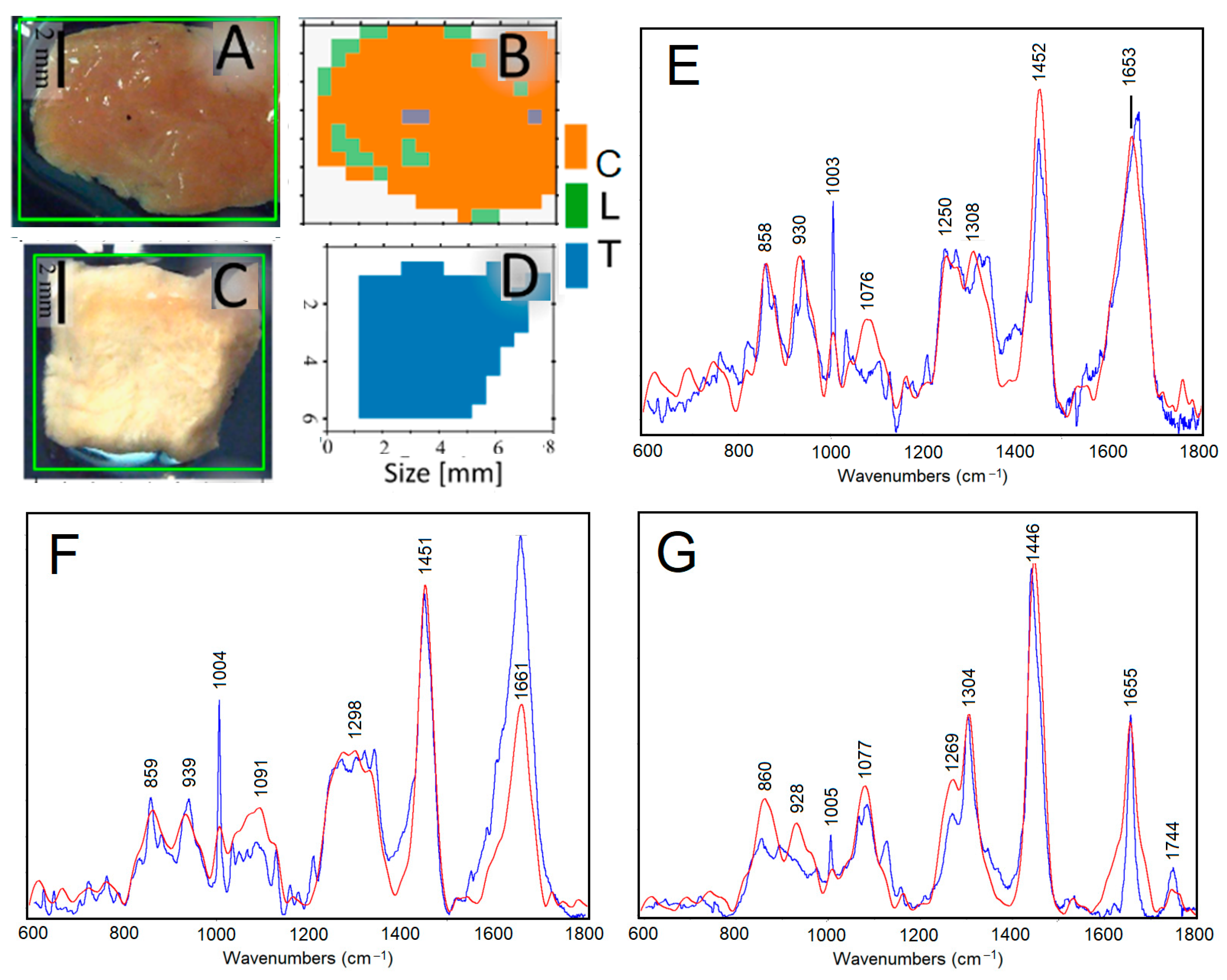
Table 1 summarizes the results of an HCA for which the KMC centroids of non-tumor and tumor samples served as input. The dendrogram of the HCA in Figure 3 arranges the centroids of 23 clusters into four groups, namely lipids—L, necrosis—N, tumor—T, and control—C. Non-tumor and tumor samples 8 and tumor sample 4 did not give usable data because of their carbon-like appearance, probably due to cauterization during surgery. It is evident from Table 1 and Figure 3 that non-tumor specimens contain beside control and lipid-rich tissue also tumor in 1 and 2, and vice versa, tumor specimens contain beside tumor and necrosis also control tissue in 7 and 10. This is consistent with the previous study and will be discussed in Section 4.

Table 1.
Assignment of cluster membership of centroid Raman spectra: control (C), necrosis (N), tumor (T), and lipid-rich tissue (L). Shaded entries are from previous work [17].
The dendrogram arranges lipid-rich tissues of non-tumor specimens 1, 2, 3, 5, 6, and 9 in a well-separated group. Necrotic tissues are identified in non-tumor specimen 3 and tumor specimens 1 and 5. Tumor tissues are found in four tumor and two non-tumor specimens and control tissue in six non-tumor and two tumor specimens.

Figure 3.
Dendrogram of hierarchical cluster analysis with k-means cluster centroids of Raman spectra as input: tumor (red), lipid (orange), necrosis (green), and control (purple) in the spectral region 800–1150 cm−1. The samples are labeled as non-tumor (N) and tumor (T) according to Table 1.
Figure 3.
Dendrogram of hierarchical cluster analysis with k-means cluster centroids of Raman spectra as input: tumor (red), lipid (orange), necrosis (green), and control (purple) in the spectral region 800–1150 cm−1. The samples are labeled as non-tumor (N) and tumor (T) according to Table 1.
3.3. Variations of Raman Spectra of Tumor and Control Tissue
Figure 4 compares the four tumor-assigned clusters in tumor specimens and six control-assigned clusters in non-tumor specimens. Control tissues tend to show more intense collagen bands near 850 and 935 cm−1 relative to the phenylalanine band at 1006 cm−1 than tumor tissue. Therefore, HCA was performed in the spectral range 800–1150 cm−1. Unspecific variations were evident for band positions and intensities in the spectral range from 1150 to 1400 cm−1. Similarly, main bands near 1450 and 1660 cm−1 did not change significantly, and the observed changes did not improve the separation of tissue classes.
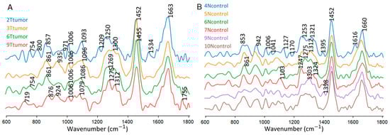
Figure 4.
Centroid Raman spectra of tumor-assigned clusters in tumor specimens (A) and control-assigned clusters in control specimens (B).
4. Discussion
Although the experimental parameters and data processing differed between 1064 nm and 785 nm Raman instruments, the main spectral findings were consistent, as shown by the summarized assignments in Table 1. Lipid and control tissues were detected in non-tumor specimen 5, and tumor was detected in tumor specimen 3, both in this work using the 1064 nm Raman probe system and in the previous work using a 785 nm Raman microscope [17]. Overall, the results from both instruments agree better for non-tumor specimens, according to Table 1, whereas discrepancies are more prevalent in tumor specimens. A difference in non-tumor 3 is the detection of necrosis at 1064 nm excitation and tumor at 785 nm. Differences in tumor 5 are related to the detection of necrosis at 1064 nm excitation and tumor, lipid, and necrosis at 785 nm, and differences in tumor 7 are the detection of control at 1064 nm and tumor at 785 nm. The discrepancies may originate from variations in sample orientations and heterogeneities, which occurred when the sample was returned to the vial after 785 nm experiments, frozen, thawed, and remounted again into the holder for the 1064 nm experiments. During intraoperative frozen section analysis, ink spots are commonly employed to mark the sample’s orientation within the resection area, minimizing ambiguities. However, the spectral contributions of the ink may interfere with the Raman results.
As a main difference between results from 1064 nm and 785 nm instruments, more tissue types are identified at 785 nm excitation. For simplicity, in Table 1, epithelial tissue, plastic, and pigment particles were not included, and they were detected at 785 nm excitation but not at 1064 nm excitation. Possible explanations are the better spectral resolution of 4 cm−1 at 785 nm (instead of 10 cm−1 here), better lateral resolution at a step size of 250 µm (instead of 400 to 500 µm here), and the vertex component analysis (VCA) algorithm. The superior discriminatory power of VCA was already demonstrated to visualize individual cell nuclei in Raman images of lung tissue [27] and 3D cell cultures [28]. KMC that was applied here failed to resolve cell nuclei in the same data sets. Another factor for the reduced discrimination ability could be the ca. twofold deeper penetration of 1064 nm light than 785 nm light that was recently quantitatively assessed [29]. Whereas deeper light penetration is beneficial for higher Raman intensities, signal detection from deeper tissue layers may result in “spectral dilution”. This term was introduced in the context of infrared imaging, where lower-resolved images failed to resolve spectral features [30]. Here, the deeper penetration of 1064 nm light tends to probe more lipids in control tissue, as evident from more intense lipid bands near 1076 and 1452 cm−1 (Figure 2E), and vice versa, more proteins in lipid-rich tissue, as evident from more intense collagen bands near 860, 928, 1269 in amide III region, and 1655 cm−1 in amide I region (Figure 2G).
The dendrograms of the HCA show for 1064 and 785 nm data that tumor forms a separate group and lipid-rich tissues are well separated from necrosis, tumor, and control. Necrosis was arranged between the tumor and lipids here, whereas necrosis overlaps with the control at 785 nm excitation. This can be explained by the selected spectral range from 800 to 1150 cm−1 here and from 800 to 1380 cm−1 in reference [17]. Tumor tissue is characterized by lower spectral contributions of collagenous proteins relative to non-collagenous proteins, which is detectable in both spectral ranges. A smaller spectral range was chosen due to unspecific variations that will be further studied in upcoming work.
In the urological context, Raman-based techniques also offer potential applications in kidney diseases [31]. Raman spectroscopy of urinary calculi was already reviewed in 1997 [32], and progress in the analysis and classification of kidney stones has recently been reported [33]. Raman spectra were used to identify cystine-type kidney stones [34], calcium-oxalate-type kidney stones [35], and phosphate-type kidney stones [36]. Kidney stones are known for their intense autofluorescence, which has even been used for experimental evaluation of human kidney stone fluorescence spectra [37]. Chemical bleaching of renal stones was one approach to reduce fluorescence in Raman spectra at 532 nm laser excitation [38]. Other approaches analyzed human urinary stones by FT–Raman [39,40] and a portable dispersive Raman system [14], both at 1064 nm excitation to suppress unwanted fluorescence background. Raman chemical imaging using a confocal Raman microspectrometer generated maps of the constituents’ distribution in a case study of structural analysis of kidney stones [41]. It was concluded that (i) a huge autofluorescence background interferes with the detection of low-concentrated and poor Raman scatterers, and (ii) this analysis is time-consuming. The Raman imaging spectrometer described here allows a faster and more sensitive way to map kidney stones due to the larger laser diameter and absence of fluorescence background. Furthermore, the lower confocality of our fiber probe instrument would facilitate the mapping of uneven stone surfaces.
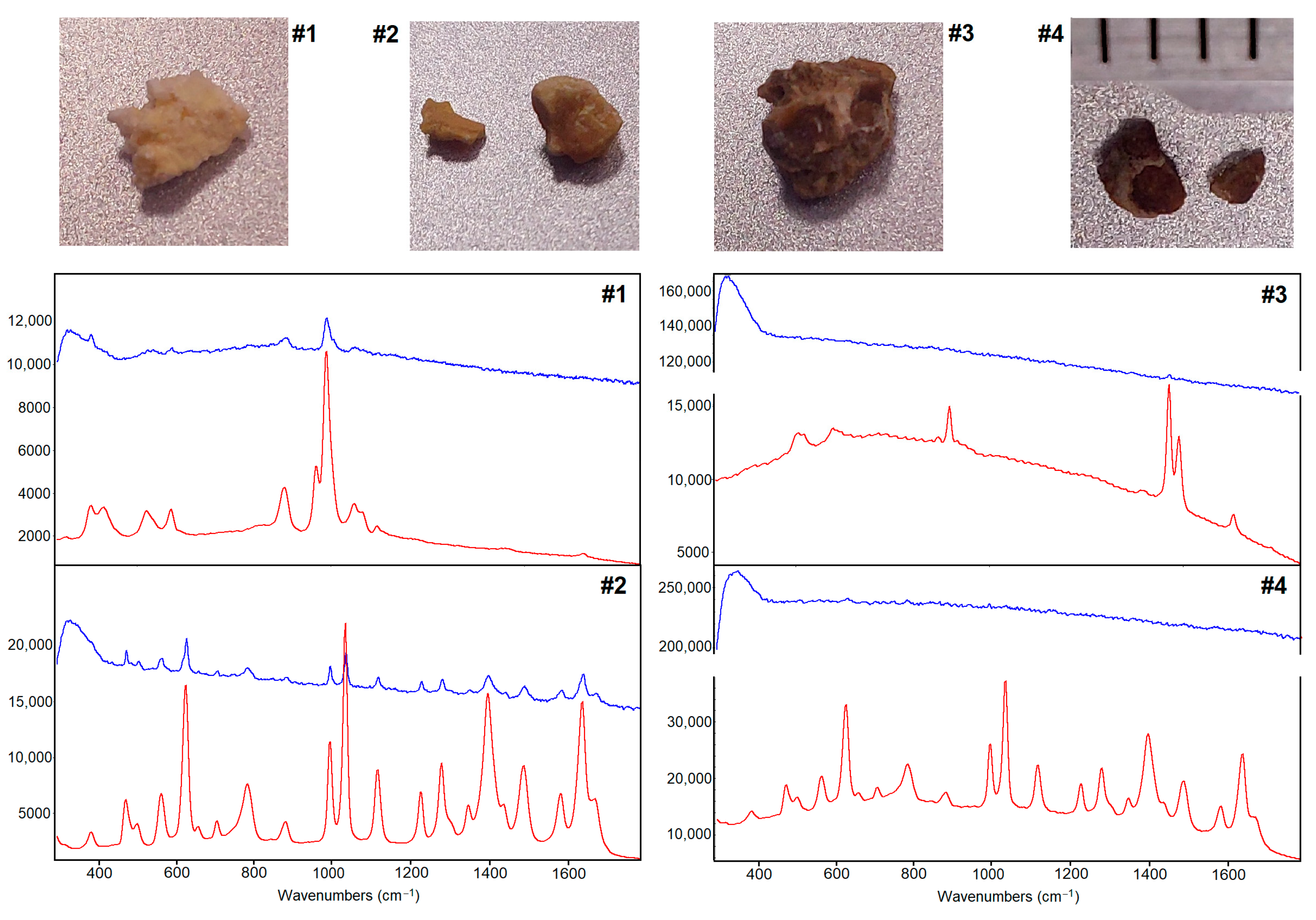
Preliminary experiments in Figure 5 compare the quality of 1064 nm excited Raman spectra of four kidney stones with 785 nm excited Raman spectra that were collected with a state-of-the-art instrument (RNX1 microprobe, Kaiser Optical System, Ann Arbor, MI, USA) used in a previous study [17]. A quantitative analysis of the signal-to-noise ratios is complicated considering the quantum efficiency and the dark noise of InGaAs versus CCD detectors, the exposure time, the laser intensity, and the wavelength−4 dependent light scattering. According to this law, the scattered band intensities are expected to decrease by a factor of 0.3 = 1064−4/785−4. Qualitative comparisons are given instead. With the same exposure time of 5 s, the better signal-to-noise ratio with the 1064 nm instrument is due to the higher laser power and enables to assign stone #1 to Ca2+ hydrogen phosphate. The intensity of the 987 cm−1 band at 450 mW of the 1064 nm laser is estimated as 8000 counts above a 2000 counts background, whereas the intensity of this band at 100 mW of the 785 nm laser (maximum power determined at the sample plane) is reduced to 2000 counts above an elevated 10,000 counts background. To avoid detector saturation, the 785 nm laser power was reduced to 25 mW, and the acquisition time was set to three exposures of 2 s for stones #2 and #3 and six exposures of 1 s for stone #4, totaling 6 s. Despite the reduced laser power, the background increases to 15,000, 100,000, and 200,000 counts for stones #2, #3, and #4, respectively. The most intense bands in stone #2 at 1649, 1037, and 628 cm−1 show ca. 3000 counts above the background, and virtually no bands are resolved in stones #3 and #4 with a darker appearance. At unchanged 1064 nm laser power and 5 s exposure time, acceptable background between 1000 and 10,000 counts and maximum band intensities between 5000 and 20,000 counts enable to assign stone #3 to Ca2+ oxalate monohydrate and stones #2 and #4 to cystine types. This clearly demonstrated the benefits of 1064 nm Raman spectroscopy, and more data will be collected in the future.
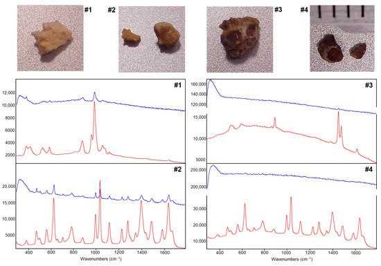
Figure 5.
Photomicrographs and Raman spectra of kidney stones at 785 nm (blue traces) and 1064 nm excitation (red traces). Unprocessed spectra are displayed at an appropriate intensity scale for comparison. The scale of a ruler in mm units in #4 is also valid for #1 to #3.
The energy deposit of inelastic light scattering in Raman spectroscopy depends on the wavelength and the absorption properties of the sample. The laser threshold, which is allowed during endoscopy to excite Raman spectra without harming tissue, is under debate [42]. An in vivo Raman study with 785 nm excitation to study atherosclerotic plaque depositions in blood vessels of a rabbit model used a fiber optic probe with a 100 µm core diameter and 100 mW laser power without a focusing element and good Raman spectra were acquired without noticeable photo-induced degradation [43]. The intensity per area using a 200 µm focus diameter and 450 mW power of a 1064 nm laser is almost equal to these conditions as the fourfold power is distributed over a four times larger area. Considering the weaker absorption of 1064 nm than 785 nm light, the risk of phototoxic effects is lower, and potential endoscopic applications are expected to be suitable with dedicated fiber probes using 450 mW power at 1064 nm excitation.
5. Conclusions
A Raman system with a 1064 nm excitation laser was coupled to a fiber probe, a digital microscope, and a motorized stage. The near-infrared excitation wavelength (λ) enabled light penetration down to several hundred micrometers. The detection by a lens with NA 0.3 in combination with a 600 µm fiber core gave poor confocality but offered extracting volumetric information from deeper tissue layers, which partly compensates for the lower scattering intensity of factor 0.3 due to the λ−4 Rayleigh law. As a consequence of the focus diameter near 200 µm, a high-precision motorized stage was not required, and an inexpensive model was selected instead with a large scan range of 200 × 300 mm. Overall, such a compact and versatile Raman instrument shows great potential for applied sciences, in particular for samples with a high fluorescent background.
The performance of the 1064 nm Raman instrument was demonstrated for non-tumor and tumor specimens of resected human bladders. Radical cystectomy is performed in patients with high-grade, muscle-invasive tumor diseases. Due to previous treatments such as endoscopic resection of non-muscle-invasive tumors and photodynamic therapy, necrosis is often present beside lipid-rich, control, and tumor tissue. Preprocessing of 1064 nm Raman images by baseline correction, smoothing, and normalization followed by processing with KMC and HCA revealed four clusters that were assigned to necrosis, lipid-rich, control, and tumor tissue. The findings agreed well with Raman images at 785 nm of these specimens. Deviations between 1064 nm and 785 nm Raman data sets might be due to different sample orientations. Proper correlation with the histopathological gold standard of parallel hematoxylin and eosin-stained tissue sections is also impaired by different orientations. Resected tissue can be stained by inks to label the orientation, e.g., to assess the tumor margin. However, these inks give intense Raman signals and/or high backgrounds that interfere with the spectral fingerprint of tissue. The 1064 nm option would be interesting for Raman imaging of intraoperative specimens with ink labels because inks do not contribute to 1064 nm excited Raman spectra. Another interesting urological application of a portable dispersive 1064 nm fiber probe Raman imaging spectrometer is the assessment of kidney stones whose Raman spectra are often affected by intense fluorescence at visible excitation wavelengths. It was shown that the identification of the stone type failed in two cases with the 785 nm Raman instrument and was successful in all cases with the 1064 nm instrument.
Author Contributions
Conceptualization, J.D.M.-B., T.A.S. and C.K.; methodology, J.D.M.-B. and T.A.S.; software, J.D.M.-B. and T.A.S.; investigation, J.D.M.-B.; resources, C.K., J.P. and A.M.; writing—original draft preparation, J.D.M.-B. and C.K.; writing—review and editing, all; supervision, C.K. and J.P.; funding acquisition, C.K. and A.M. All authors have read and agreed to the published version of the manuscript.
Funding
This work has partially been funded by the German Federal Ministry of Education and Research (BMBF) under the project UroMDD (03ZZ0444).
Institutional Review Board Statement
The study was conducted in accordance with the Declaration of Helsinki and approved by the Institutional Ethics Committee) of the University of Freiburg (protocol code 592/17 (191723) approved on 30 January 2020) for studies involving humans.
Informed Consent Statement
Informed consent was obtained from all subjects involved in the study.
Data Availability Statement
The raw data supporting the conclusions of this article will be made available by the authors on request.
Acknowledgments
The authors thank Peter Bronsert (Faculty of Medicine, University Freiburg, Germany) for support in providing bladder specimens.
Conflicts of Interest
The authors declare no conflicts of interest.
References
- Heidkamp, J.; Scholte, M.; Rosman, C.; Manohar, S.; Fütterer, J.J.; Rovers, M.M. Novel imaging techniques for intraoperative margin assessment in surgical oncology: A systematic review. Int. J. Cancer 2021, 149, 635–645. [Google Scholar] [CrossRef]
- Krafft, C.; Popp, J. Opportunities of optical and spectral technologies in intraoperative histopathology. Optica 2023, 10, 214–231. [Google Scholar] [CrossRef]
- Lee, M.; Herrington, C.S.; Ravindra, M.; Sepp, K.; Davies, A.; Hulme, A.N.; Brunton, V.G. Recent advances in the use of stimulated raman scattering in histopathology. Analyst 2021, 146, 789–802. [Google Scholar] [CrossRef]
- Zhang, C.; Aldana-Mendoza, J.A. Coherent raman scattering microscopy for chemical imaging of biological systems. J. Phys. Photonics 2021, 3, 032002. [Google Scholar] [CrossRef]
- Kögler, M.; Heilala, B. Time-gated raman spectroscopy—A review. Meas. Sci. Technol. 2020, 32, 012002. [Google Scholar] [CrossRef]
- Korinth, F.; Shaik, T.A.; Popp, J.; Krafft, C. Assessment of shifted excitation raman difference spectroscopy in highly fluorescent biological samples. Analyst 2021, 146, 6760–6767. [Google Scholar] [CrossRef]
- Sowoidnich, K.; Towrie, M.; Maiwald, M.; Sumpf, B.; Matousek, P. Shifted excitation raman difference spectroscopy with charge-shifting charge-coupled device (ccd) lock-in detection. Appl. Spectrosc. 2019, 73, 1265–1276. [Google Scholar] [CrossRef] [PubMed]
- Kozik, A.; Pavlova, M.; Petrov, I.; Bychkov, V.; Kim, L.; Dorozhko, E.; Cheng, C.; Rodriguez, R.D.; Sheremet, E. A review of surface-enhanced raman spectroscopy in pathological processes. Anal. Chim. Acta 2021, 1187, 338978. [Google Scholar] [CrossRef] [PubMed]
- Langer, J.; Jimenez de Aberasturi, D.; Aizpurua, J.; Alvarez-Puebla, R.A.; Auguié, B.; Baumberg, J.J.; Bazan, G.C.; Bell, S.E.; Boisen, A.; Brolo, A.G. Present and future of surface-enhanced raman scattering. ACS Nano 2019, 14, 28–117. [Google Scholar] [CrossRef]
- Ye, J.; Tian, Z.; Wei, H.; Li, Y. Baseline correction method based on improved asymmetrically reweighted penalized least squares for the raman spectrum. Appl. Opt. 2020, 59, 10933–10943. [Google Scholar] [CrossRef]
- Barton, B.; Thomson, J.; Lozano Diz, E.; Portela, R. Chemometrics for raman spectroscopy harmonization. Appl. Spectrosc. 2022, 76, 1021–1041. [Google Scholar] [CrossRef]
- Schrader, B.; Dippel, B.; Fendel, S.; Keller, S.; Löchte, T.; Riedl, M.; Schulte, R.; Tatsch, E. Nir ft raman spectroscopy—a new tool in medical diagnostics. J. Mol. Struct. 1997, 408–409, 23–31. [Google Scholar] [CrossRef]
- Chao, K.; Dhakal, S.; Qin, J.; Kim, M.; Peng, Y. A 1064 nm dispersive raman spectral imaging system for food safety and quality evaluation. Appl. Sci. 2018, 8, 431. [Google Scholar] [CrossRef]
- Zhu, W.; Sun, Z.; Ye, L.; Zhang, X.; Xing, Y.; Zhu, Q.; Yang, F.; Jiang, G.; Chen, Z.; Chen, K.; et al. Preliminary assessment of a portable raman spectroscopy system for post-operative urinary stone analysis. World J. Urol. 2022, 40, 229–235. [Google Scholar] [CrossRef]
- Worldwide Cancer Data. Available online: https://www.wcrf.org/cancer-trends/worldwide-cancer-data (accessed on 12 January 2024).
- Lenis, A.T.; Lec, P.M.; Chamie, K. Bladder cancer: A review. JAMA 2020, 324, 1980–1991. [Google Scholar] [CrossRef]
- Krafft, C.; Popp, J.; Bronsert, P.; Miernik, A. Raman spectroscopic imaging of human bladder resectates towards intraoperative cancer assessment. Cancers 2023, 15, 2162. [Google Scholar] [CrossRef]
- Cordero, E.; Rüger, J.; Marti, D.; Mondol, A.S.; Hasselager, T.; Mogensen, K.; Hermann, G.G.; Popp, J.; Schie, I.W. Bladder tissue characterization using probe-based raman spectroscopy: Evaluation of tissue heterogeneity and influence on the model prediction. J. Biophotonics 2020, 13, e201960025. [Google Scholar] [CrossRef]
- Yang, M.; Wang, J.; Quan, S.; Xu, Q. High-precision bladder cancer diagnosis method: 2D raman spectrum figures based on maintenance technology combined with automatic weighted feature fusion network. Anal. Chim. Acta 2023, 1282, 341908. [Google Scholar] [CrossRef]
- Liu, Y.; Ye, F.; Yang, C.; Jiang, H. Use of in vivo raman spectroscopy and cryoablation for diagnosis and treatment of bladder cancer. Spectrochim. Acta Part A Mol. Biomol. Spectrosc. 2024, 308, 123707. [Google Scholar] [CrossRef] [PubMed]
- Munoz-Bolanos, J.D.; Shaik, T.A.; Popp, J.; Krafft, C. Hyperspectral Package for Spectroscopists (Spectramap). 2021. Available online: https://pypi.org/project/spectramap/ (accessed on 14 January 2024).
- Zhang, Z.-M.; Chen, S.; Liang, Y.-Z. Baseline correction using adaptive iteratively reweighted penalized least squares. Analyst 2010, 135, 1138–1146. [Google Scholar] [CrossRef] [PubMed]
- Schafer, R.W. What is a savitzky-golay filter? [lecture notes]. IEEE Signal Process. Mag. 2011, 28, 111–117. [Google Scholar] [CrossRef]
- Ospanov, A.; Romanishkin, I.; Savelieva, T.; Kosyrkova, A.; Shugai, S.; Goryaynov, S.; Pavlova, G.; Pronin, I.; Loschenov, V. Optical differentiation of brain tumors based on raman spectroscopy and cluster analysis methods. Int. J. Mol. Sci. 2023, 24, 14432. [Google Scholar] [CrossRef]
- Schie, I.W.; Krafft, C.; Popp, J. Cell classification with low-resolution raman spectroscopy (lrrs). J. Biophotonics 2016, 9, 994–1000. [Google Scholar] [CrossRef]
- Kumamoto, Y.; Mochizuki, K.; Hashimoto, K.; Harada, Y.; Tanaka, H.; Fujita, K. High-throughput cell imaging and classification by narrowband and low-spectral-resolution raman microscopy. J. Phys. Chem. B 2019, 123, 2654–2661. [Google Scholar] [CrossRef] [PubMed]
- Krafft, C.; Alipour Didehroshan, M.; Recknagel, P.; Miljkovic, M.; Bauer, M.; Popp, J. Crisp and soft algorithms visualizes cell nuclei in raman images of liver tissue sections. Vib. Spectrosc. 2011, 55, 90–100. [Google Scholar] [CrossRef]
- Kallepitis, C.; Bergholt, M.S.; Mazo, M.M.; Leonardo, V.; Skaalure, S.C.; Maynard, S.A.; Stevens, M.M. Quantitative volumetric raman imaging of three dimensional cell cultures. Nat. Commun. 2017, 8, 14843. [Google Scholar] [CrossRef]
- Lin, L.; He, H.; Xue, R.; Zhang, Y.; Wang, Z.; Nie, S.; Ye, J. Direct and quantitative assessments of near-infrared light attenuation and spectroscopic detection depth in biological tissues using surface-enhanced raman scattering. Med-X 2023, 1, 9. [Google Scholar] [CrossRef]
- Lasch, P.; Naumann, D. Spatial resolution in infrared microspectroscopic imaging of tissues. Biochim. Biophys. Acta (BBA)—Biomembr. 2006, 1758, 814–829. [Google Scholar] [CrossRef] [PubMed]
- Delrue, C.; Speeckaert, M.M. The potential applications of raman spectroscopy in kidney diseases. J. Pers. Med. 2022, 12, 1644. [Google Scholar] [CrossRef]
- Carmona, P.; Bellanato, J.; Escolar, E. Infrared and raman spectroscopy of urinary calculi: A review. Biospectroscopy 1997, 3, 331–346. [Google Scholar] [CrossRef]
- Cui, X.; Zhao, Z.; Zhang, G.; Chen, S.; Zhao, Y.; Lu, J. Analysis and classification of kidney stones based on raman spectroscopy. Biomed. Opt. Express 2018, 9, 4175–4183. [Google Scholar] [CrossRef] [PubMed]
- Kodati, V.R.; Tu, A.T. Raman spectroscopic identification of cystine-type kidney stone. Appl. Spectrosc. 1990, 44, 837–839. [Google Scholar] [CrossRef]
- Kodati, V.R.; Tomasi, G.E.; Turumin, J.L.; Tu, A.T. Raman spectroscopic identification of calcium-oxalate-type kidney stone. Appl. Spectrosc. 1990, 44, 1408–1411. [Google Scholar] [CrossRef]
- Kodati, V.R.; Tomasi, G.E.; Turumin, J.L.; Tu, A.T. Raman spectroscopic identification of phosphate-type kidney stones. Appl. Spectrosc. 1991, 45, 581–583. [Google Scholar] [CrossRef]
- Schütz, J.; Miernik, A.; Brandenburg, A.; Schlager, D. Experimental evaluation of human kidney stone spectra for intraoperative stone-tissue-instrument analysis using autofluorescence. J. Urol. 2019, 201, 182–188. [Google Scholar] [CrossRef] [PubMed]
- Kocademir, M.; Kumru, M.; Gölcük, K.; Suarez-Ibarrola, R.; Miernik, A. Fluorescence reduction in raman spectroscopy by chemical bleaching on renal stones. J. Appl. Spectrosc. 2020, 87, 282–288. [Google Scholar] [CrossRef]
- Selvaraju, R.; Raja, A.; Thiruppathi, G. Ft-raman spectral analysis of human urinary stones. Spectrochim. Acta Part A Mol. Biomol. Spectrosc. 2012, 99, 205–210. [Google Scholar] [CrossRef]
- Tonannavar, J.; Deshpande, G.; Yenagi, J.; Patil, S.B.; Patil, N.A.; Mulimani, B.G. Identification of mineral compositions in some renal calculi by ft raman and ir spectral analysis. Spectrochim. Acta Part A Mol. Biomol. Spectrosc. 2016, 154, 20–26. [Google Scholar] [CrossRef]
- Castiglione, V.; Sacré, P.-Y.; Cavalier, E.; Hubert, P.; Gadisseur, R.; Ziemons, E. Raman chemical imaging, a new tool in kidney stone structure analysis: Case-study and comparison to fourier transform infrared spectroscopy. PLoS ONE 2018, 13, e0201460. [Google Scholar] [CrossRef]
- Galli, R.; Uckermann, O.; Andresen, E.F.; Geiger, K.D.; Koch, E.; Schackert, G.; Steiner, G.; Kirsch, M. Intrinsic indicator of photodamage during label-free multiphoton microscopy of cells and tissues. PLoS ONE 2014, 9, e110295. [Google Scholar] [CrossRef]
- Matthäus, C.; Dochow, S.; Bergner, G.; Lattermann, A.; Romeike, B.; Marple, E.; Krafft, C.; Dietzek, B.; Brehm, B.; Popp, J. In vivo characterization of atherosclerotic plaque depositions by raman-probe spectroscopy and in vitro cars microscopic imaging on a rabbit model. Anal. Chem. 2012, 84, 7845–7851. [Google Scholar] [CrossRef] [PubMed]


Disclaimer/Publisher’s Note: The statements, opinions and data contained in all publications are solely those of the individual author(s) and contributor(s) and not of MDPI and/or the editor(s). MDPI and/or the editor(s) disclaim responsibility for any injury to people or property resulting from any ideas, methods, instructions or products referred to in the content. |
© 2024 by the authors. Licensee MDPI, Basel, Switzerland. This article is an open access article distributed under the terms and conditions of the Creative Commons Attribution (CC BY) license (https://creativecommons.org/licenses/by/4.0/).