Abstract
Lightweight LiDAR, characterized by its ease of use and cost-effectiveness, offers advantages in road intersection information acquisition. This study used lightweight LiDAR to collect 3D point cloud data from an urban road intersection and propose a semantic segmentation model based on the improved RandLA-Net. Initially, raw data from multiple positions and perspectives were obtained, and complete road intersection point clouds were stitched together using the iterative closest point algorithm for sequential registration. Subsequently, a semantic segmentation method for point clouds based on the improved RandLA-Net was proposed. This method included a spatial information encoding module based on feature similarities and a feature enhancement module based on multi-pooling fusion. This model optimized the feature aggregation capabilities during downsampling with the weighted cross-entropy loss function applied to reduce the impact of input sample scale imbalances. In comparisons of the improved RandLA-Net with PointNet++ and RandLA-Net on the same dataset, our method showed improved segmentation accuracy for various categories. The overall prediction accuracy on two road intersection point cloud test sets was 87.68% and 89.61%, with average F1 scores of 82.76% and 80.61%, respectively. Most notably, the prediction accuracy for road surface areas reached 94.48% and 94.79%. The results show that our model can enrich the spatial feature expression of input data and enhance semantic segmentation performance in road intersection scenarios.
1. Introduction
With the development of digital road mapping technology, 3D scanning technology based on light detection and ranging (LiDAR) has shown promising prospects in the management of road infrastructures [1,2]. As crucial components of the road traffic system [3], road intersections offer significant value in extracting information. Urban road intersections encompass a variety of ancillary facilities, including traffic lights, drainage, lighting, and greening facilities [4], creating challenges for data collection using LiDAR. Lightweight LiDAR, characterized by its ease of operation, cost-effectiveness, and strong environmental adaptability, employs non-repetitive scanning methods and fewer sensors [5], thereby simplifying the complex and time-consuming multi-beam laser calibration process. Compared to vehicle-mounted LiDAR and airborne LiDAR, lightweight LiDAR typically uses a static installation that is unaffected by the movement of the vehicle or aircraft, resulting in more stable data acquisition. In addition, given the complexity of the facilities, vehicles, and pedestrians at road intersections, lightweight LiDAR can avoid irrelevant factors affecting data quality by acquiring multi-angle point cloud data.
The complexity of road intersections places high demands on the performance of semantic segmentation methods. Traditional point cloud semantic segmentation methods often employ supervised learning algorithms that use, for example, attribute clustering [6,7,8], model fitting [9], and region growing [10,11,12,13]. However, the segmentation accuracy of these algorithms is usually limited by manually set experience thresholds, making them unsuitable for the complex and variable scenarios of road intersections. In recent years, many scholars have achieved promising results in semantic segmentation using deep learning methods [14] on multiple public point cloud datasets [15,16].
Artificial neural networks with multiple overlapping hidden layers possess strong feature learning capabilities [17]. Artificial neural networks project point clouds into a grid structure, converting raw data into 2D images [18,19] or 3D voxels for processing [20,21], with segmentation outcomes heavily dependent on the data quality of point clouds from different perspectives (e.g., mutual occlusion). This method also struggles to balance feature completeness with computational resource consumption [22], making it unsuitable for the semantic segmentation of road scene point clouds. Point-based semantic segmentation methods, on the other hand, directly use point clouds as network inputs for end-to-end spatial feature learning [23] with strong robustness and generalization capabilities. For processing large-scale, multi-category point cloud scenes, networks such as RandLA-Net [24], BAAF-Net [25], and SCF-Net [26] often employ random sampling methods with low computational complexity and high storage efficiency. Despite the introduction of structures to capture local features, the sparse distribution and uneven granularity of downsampled point clouds still affect model training effectiveness. The BAF-LAC network [27], building on the RandLA-Net framework, introduced a backward attention fusion mechanism and a local aggregation classifier, thereby enhancing point cloud classification accuracy. However, large-scale point cloud semantic segmentation models continue to face challenges in fully expressing features, particularly in terms of segmentation performance in road intersection scenarios.
The method proposed in this study uses lightweight LiDAR for point cloud data collection at road intersections. After preprocessing steps such as registration stitching and data simplification, we implement a semantic segmentation method for point clouds based on an improved RandLA-Net. We also introduce an enhanced feature aggregation module incorporating a spatial information encoding layer, a pooling layer, and a dilated residual layer to strengthen key feature information in the point cloud and thus avoid losing this useful information during model downsampling. In this module’s spatial information encoding layer, a feature similarity matrix is constructed to output the neighborhood spatial information of each sampled point. This matrix is then fused through a pooling operation. Finally, a weighted cross-entropy loss function is set to optimize the network’s training effectiveness in road intersection scenarios.
2. Materials and Methods
2.1. Point Cloud Data Collection
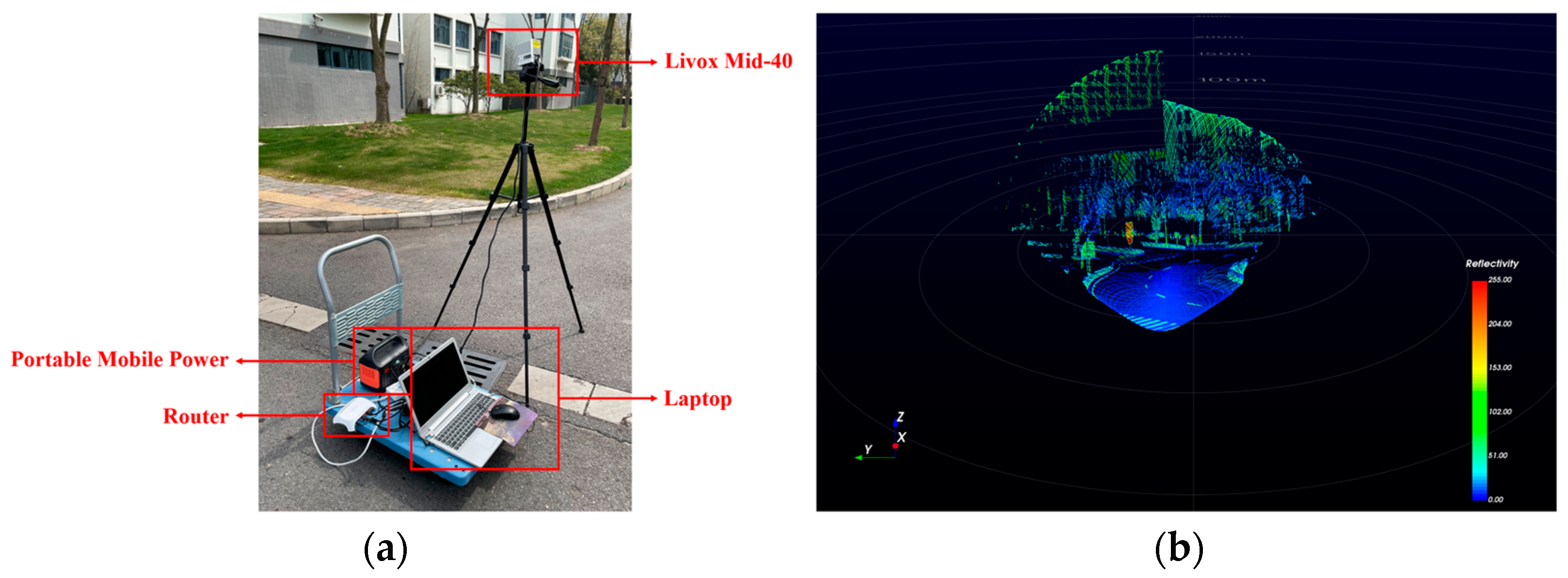
The lightweight laser scanning system consists of a scanning system (LiDAR), a control system, and a computer system [28]. During the collection of road point cloud data, lightweight LiDAR usually employs a static setup for measurements and is unable to move or rotate during a single scan, as illustrated in Figure 1. Due to the limitations of the measuring environment and the device’s field of view, it is necessary to establish multiple survey stations. After a single scan at the same station, the LiDAR is rotated to acquire point clouds from different field angles for subsequent stitching into complete road point cloud data.
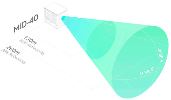
Figure 1.
Schematic diagram of lightweight LiDAR.
A Livox Mid-40 LiDAR sensor was used to collect point cloud data from typical urban road intersections. The main technical parameters are provided in Table 1 and Figure 1.

Table 1.
Livox Mid-40 LiDAR sensor main technical parameters.
2.2. Point Cloud Registration and Stitching
2.2.1. Principles of Point Cloud Registration and Stitching
The essence of point cloud registration and stitching is to perform coordinate transformation on original data, unifying the local point clouds into an overall coordinate system [29].
Let P and Q respectively represent the source and target point clouds to be registered. The process of rigid transformation in a three-dimensional space can be described as Q = R × P + T, where R is the rotation matrix and T is the translation matrix.
It should be noted that the stitching based on rotation and translation is based on the recognition of feature points. Let the source point set be and the target point set be . Any pair of feature points pi and qi should satisfy the following rigid transformation relationship:
The rotation matrix R and translation matrix T are respectively represented by the following equations:
where α, β, and γ are the rotation angles of the x, y, and z axes in the local spatial coordinate system of the point cloud, respectively, and tx, ty, and tz are the translation changes of the coordinate axes along their respective directions.
It is necessary to solve for the optimal rotation and translation parameters, that is, α, β, γ, tx, ty, and tz. To determine a unique solution, at least six linear equations must be established, meaning at least three sets of non-collinear feature point pairs must be found between the source and target point clouds to solve the system of equations. Additionally, selecting as many non-collinear feature point pairs as possible can effectively improve the computational accuracy of the system of equations, enhancing the point cloud registration effect.
To maximize the overlap of identical areas between the source and target point clouds, the model constraint can be expressed as the sum of the minimal distances between each set of feature points. Let the rigid transformation matrix be (R, T) and establish a target function to reflect the root mean square (RMS) value of the distance error for each set of feature point pairs:
where feature point pairs pi and qi respectively come from source point set P and target point set Q, and n is the number of feature point pairs.
2.2.2. Iterative Closest Point (ICP) Registration Algorithm
The iterative closest point (ICP) algorithm [30] seeks to find a solution to aligning two point clouds. Specifically, it aims to determine the optimal rigid transformation (including both rotation and translation) that minimizes the distance between corresponding points in the two point clouds.
The process involves (1) identifying the closest point in the target point set for each point in the source point set and forming feature point pairs and (2) solving for the optimal mapping transformation matrix between the source and target point clouds to ensure the best match under the constraint conditions.
The main steps of the ICP algorithm are as follows:
- Step 1: In the KD-tree data indexing structure, create feature point pairs and in source point set P and target point set Q.
- Step 2: Based on the three-dimensional spatial information of the feature point pairs, solve for the corresponding rotation parameters R and translation parameters T.
- Step 3: Perform coordinate transformation on the source point set using these parameters. If the root mean square (RMS) distance between the transformed point set and the target point set is less than the pre-set threshold, the iteration terminates; otherwise, repeat the iteration until the result meets the threshold or the maximum number of computations is reached.
- Step 4: Calculate the optimal transformation parameters and use the mapping transformation matrix to stitch the point cloud data.
2.3. Point Cloud Semantic Segmentation Model
2.3.1. Overall Network Architecture
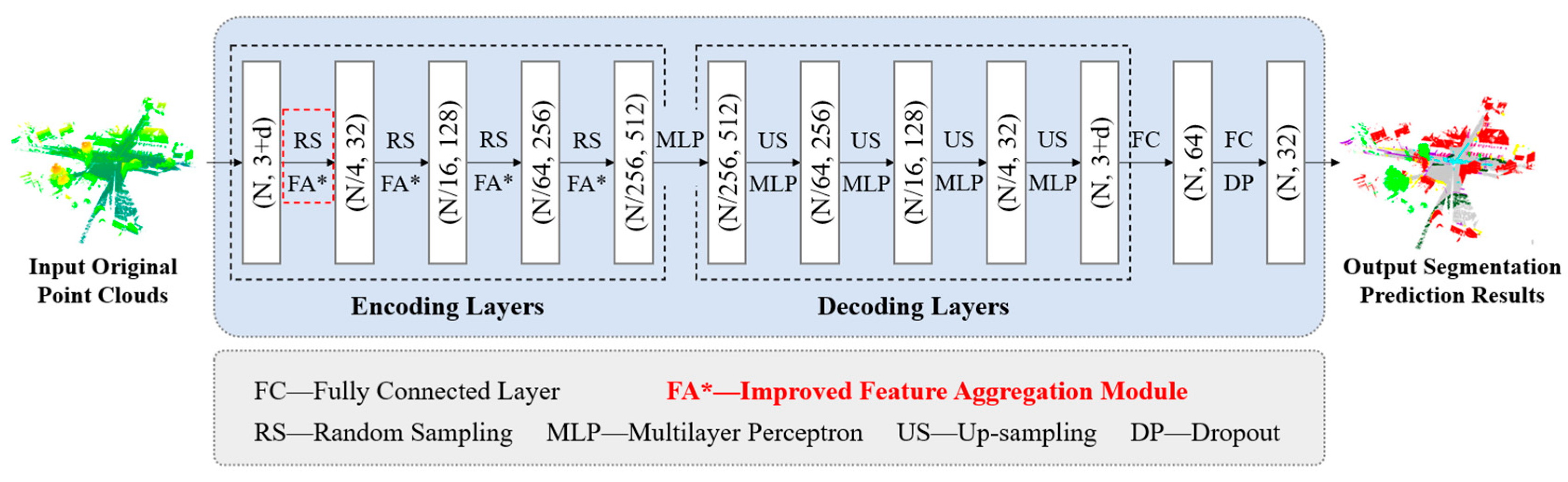
This study performs point cloud semantic segmentation based on the improved RandLA-Net, adhering to the encoder–decoder framework, as shown in Figure 2. In the encoding layers, successive random downsampling (RS) layers are applied to save computational resources and input into an improved feature aggregation module (FA*) to gradually increase the feature dimensions of each point and enrich key feature information. In the decoding layers, nearest neighbor interpolation is used to upsample (US) point cloud feature matrices, adopting the nearest neighborhood point features as features for each point. That is, upsampling operations recover higher-resolution feature matrices from lower-resolution ones. Skip link concatenation is used to cascade the upsampling results with the features obtained during the encoding stage. The results are then input into the MLP (multilayer perceptron), thus merging the features before and after sampling and restoring the dimensions of the input point cloud. Finally, through three shared fully connected (FC) layers and a dropout layer, the predicted semantic labels for the point cloud are output.

Figure 2.
The overall architecture of improved RandLA-Net.
The original input point cloud is denoted as . The features of the input point cloud include (1) positional features and (2) other features such as color and intensity. In these expressions, P represents the input point cloud, N is the number of input points, and 3 + d is the feature dimension of the input point cloud.
The feature dimensions in Figure 2 are explained below:
- (N, 3+d): The input original point clouds with N points, each having 3 + d feature dimensions.
- (N/4, 32): After random sampling (RS), the number of points is reduced to N/4, with each point having 32 feature dimensions.
- (N/16, 128): Further reduction in the number of points to N/16 with 128 feature dimensions after additional sampling and feature aggregation (FA*).
- (N/64, 256): Points are reduced to N/64 with 256 feature dimensions.
- (N/256, 512): Points are reduced to N/256 with 512 feature dimensions at the deepest encoding layer.
- (N/64, 256), (N/16, 128), (N/4, 32), (N, 3+d): The upsampling (US) layers increase the number of points back to their original count, restoring them to their respective feature dimensions during the decoding process.
2.3.2. Improved Feature Aggregation Module
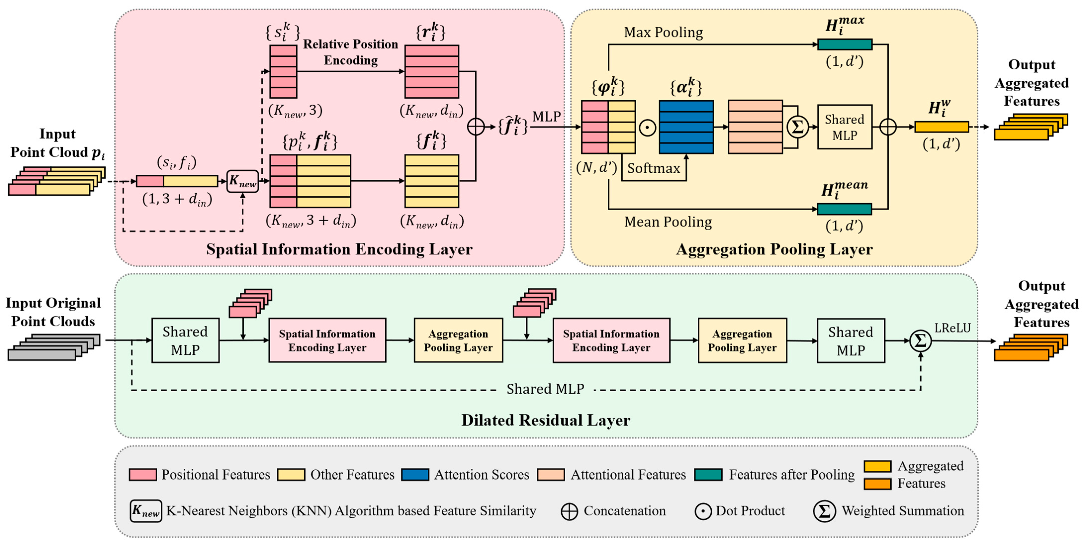
RandLA-Net’s random sampling method significantly reduces memory usage. However, due to the non-uniform distribution of 3D point clouds in space, random sampling may not accurately retain the geometric features of the point cloud, potentially resulting in a loss of effective information during downsampling. To enhance the model’s feature learning capabilities, we improve upon the original network’s local feature aggregation module (LFA), resulting in an improved feature aggregation module composed of a spatial information encoding layer, an aggregation pooling layer, and a dilated residual layer. The architecture of the improved feature aggregation module is shown in Figure 3.

Figure 3.
The architecture of the improved feature aggregation module (FA*).
(1) Spatial Information Encoding Layer: This layer explicitly encodes the coordinate information of the point cloud, allowing the network to learn the local spatial structure of the original point cloud from the relative distances and positional relationships between points. For each central sampling point, the original network uses the K-nearest neighbors (KNN) algorithm to select several of the closest points to enhance their features for describing the local spatial features of the central point. The KNN algorithm is essentially a non-parametric, instance-based learning method used for classification and regression tasks. It operates on the principle that data points with similar attributes are likely to be close together in feature space. However, points close in space to the central point may not share similar feature information, especially at the boundaries between different categories of point clouds. Consequently, such points may misrepresent local features and hinder the model’s ability to capture the point cloud’s spatial structure, as illustrated in Figure 4.
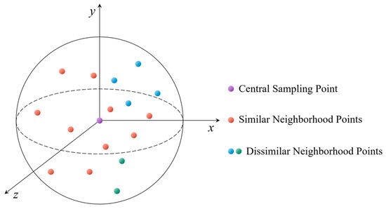
Figure 4.
Diagram of neighborhood selection for the center point in KNN.
The steps for the spatial information encoding layer are as follows:
- Step 1: Establishing Neighborhood Point Sets
Using the K-nearest neighbors (KNN) algorithm, calculate the Euclidean distance from each point in the point cloud to the central sampling points. For each central sampling point, select the K-closest neighborhood points, denoted as .
- Step 2: Constructing the Feature Similarity Matrix
Taking the central point as an example, the difference between and its neighborhood point is represented by the differences in their feature vectors (including color and intensity):
where and are the feature vectors corresponding to and , respectively. The smaller the is, the higher the similarity of features is between that and the central point .
Repeat the above process for K neighborhood points to construct a feature similarity matrix (K × 1). According to the matrix, select the Knew neighborhood points with the highest similarity to each central point, denoted as .
- Step 3: Relative Position Encoding
To enrich local spatial information, explicitly encode the relative position of the point cloud based on the similar neighborhood point set . Then, concatenate the coordinates of the central point , the coordinates of the neighborhood points , and their Euclidean distances to obtain the relative position feature. This process can be represented as follows:
where denotes the concatenation of feature matrices of the same dimension.
- Step 4: Neighborhood Feature Enhancement
For each neighborhood point of the central points, concatenate its corresponding feature with the relative position feature to obtain the enhanced feature vector . Then, the output via the multi-layer perceptron (MLP) is the relative position feature enhanced feature :
The output of the spatial information encoding unit is the neighborhood feature of each central sampling point. This information is encoded in a matrix that captures the local semantic structure of each central point, effectively enhancing the neighborhood spatial features of the input point cloud.
(2) Aggregation Pooling Layer: This layer retains the attention mechanism of the original network and enhances the point cloud features based on multi-pooling fusion.
Firstly, the maximum pooling function Hmax and the average pooling function Hmean are used, respectively, to obtain global features of each point and local features within their neighborhood. Secondly, a shared function, g(), consisting of an MLP with shared weights W and a Softmax activation function, is established to learn individual attention scores for each point:
Weighted summation is employed to aggregate the neighborhood features, as follows:
Finally, the results of the maximum pooling, average pooling, and high-dimensional features output by attention pooling are concatenated:
This result encompasses both local and global information in the point cloud, enabling the model to more accurately capture the input point cloud’s spatial structure.
(3) Dilated Residual Layer: To balance model computational efficiency and information richness when downsampling large-scale input point clouds, it is necessary to progressively expand the receptive field of each central sampling point to cover the key semantic features of the original point cloud. The network’s dilated residual layer stacks the spatial information encoding layer and aggregation pooling layer twice to increase the effective spatial range of central points in the neighborhood.
2.3.3. Loss Function Design
RandLA-Net employs a cross-entropy loss function to constrain the model’s learning characteristics using the prediction errors of individual samples. The composition of categories in road intersection scenarios is diverse, and the sample count of each category within the point cloud dataset fed into the network is imbalanced. Thus, using the original loss function may lead the model to learn the sample ratio and other prior information in the training set, giving it bias towards categories with a higher number of samples during prediction.
To ensure that the samples in each category contribute relatively equally to the loss function, a weighted cross-entropy loss function [31] is established, assigning weight coefficients to each category according to the size of the sample pool:
where ni is the number of points in the ith category, ri is the proportion of the ith category in the total number of point clouds across all categories, wi is the weight coefficient for the ith category, and nclass is the number of categories on which the model is trained.
The expression for the weighted cross-entropy loss function Lw is as follows:
where yi is the one-hot vector encoding of the ith category, and is the predicted probability of the model for the ith category.
3. Results
3.1. Data Collection and Preprocessing
3.1.1. Data Collection
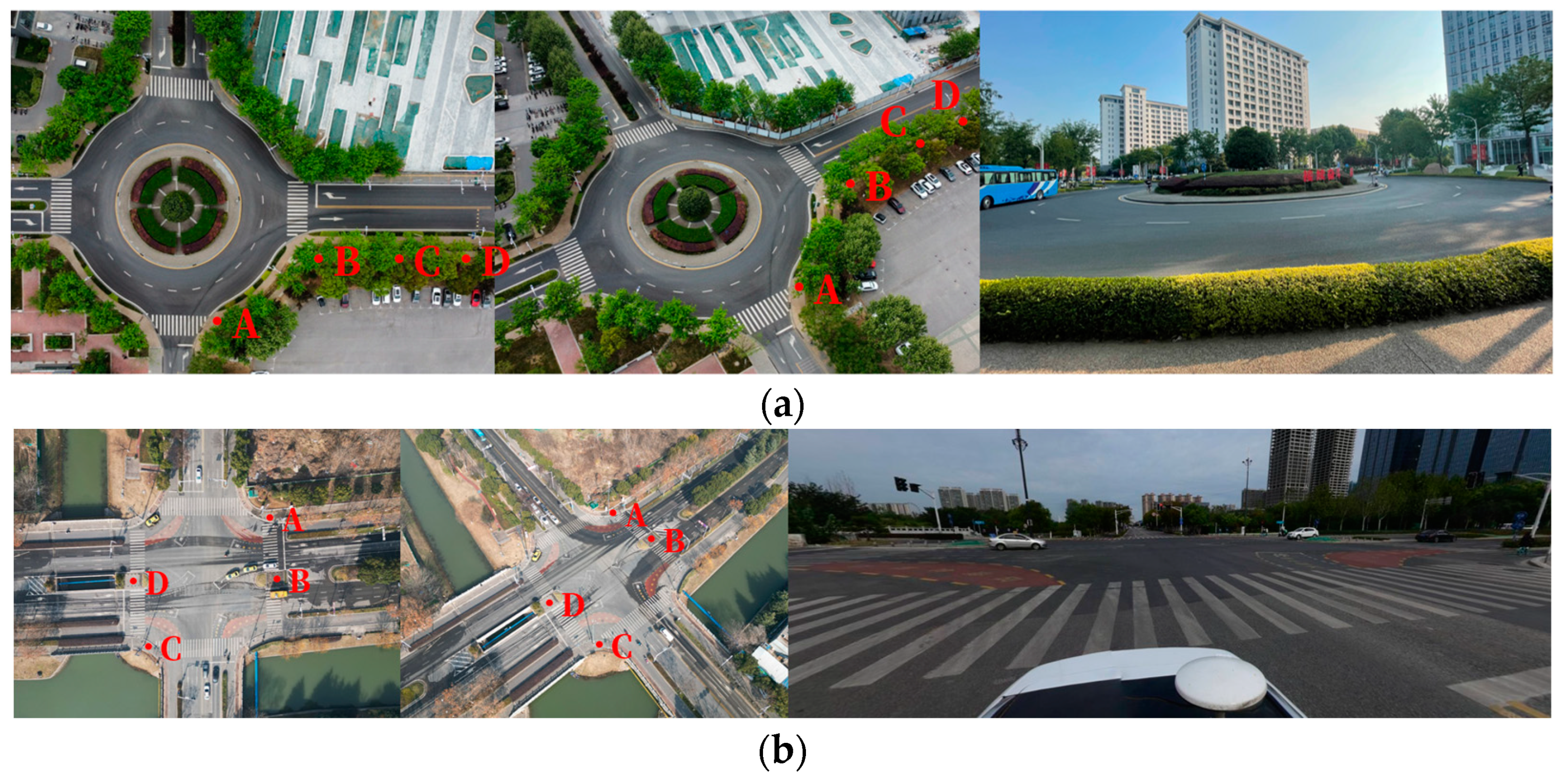
Two urban road intersections, a roundabout and a cross intersection, were selected for this study, as shown in Figure 5. Due to the limited field of view of lightweight LiDAR, the location and number of survey stations were determined based on the actual scene. The positions of the survey stations for the two experimental areas are shown in Figure 5a,b as A, B, C, and D.
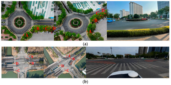
Figure 5.
Location of stations in the test area. (a) Roundabout intersection. (b) Cross intersection.
The selection criteria for the survey points were as follows:
(1) The survey points were selected in relatively safe areas within the intersection, such as pavements, to minimize the impact of traffic.
(2) The point cloud data collected from multiple survey points should collectively cover the entire intersection as comprehensively as possible.
During the data collection for the roundabout intersection, some areas were under construction, making it difficult to set up the LiDAR system. As a result, the survey points are distributed on one side of the intersection.
Additionally, data collection is typically conducted during low-traffic hours of the day. The Livox Mid-40 LiDAR (Livox Technology Company Limited, Shenzhen, China) has a limited field of view (Section 2.1); thus, efforts were made to avoid situations where vehicles were in the field of view. This approach fundamentally reduces the impact of vehicle noise on data processing, highlighting one of the advantages of using lightweight LiDAR. The data collection process is shown in Figure 6.
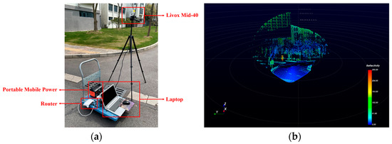
Figure 6.
Test data collection process. (a) Livox Mid-40 LiDAR scanning system. (b) Real-time acquisition screen.
3.1.2. Data Preprocessing
The method in this study implements registration and stitching of the original point clouds based on a sequential registration strategy. Here, a local coordinate system of a particular point cloud segment is used as the reference coordinate system, and then all spatial point clouds are transformed into this reference system. To enhance the reliability of the alignment results, pairs of feature points with obvious geometric spatial characteristics are selected, such as points in traffic signs, zebra crossings, and guidelines. The aforementioned process is shown in Figure 7.
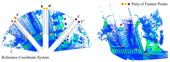
Figure 7.
Schematic of point cloud alignment stitching.
The ICP algorithm was set to run for 100 iterations, with an error threshold of 0.03 between consecutive iterations. The farthest points allowed during the iteration process were automatically removed. The distance error of feature point pairs during point cloud registration yielded the maximum RMS, minimum RMS, and average RMS values, as shown in Table 2.
Table 2.
Root mean square (RMS) of alignment errors for the intersection point cloud.
The complete point cloud data obtained after registration and data simplification are shown in Table 3 and Figure 8.
Table 3.
Basic information on the experimental data.
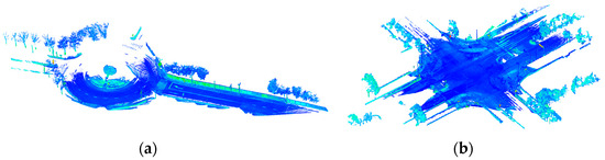
Figure 8.
Full point cloud renderings of the road intersections. (a) Set 1. (b) Set 2.
3.2. Experimental Data and Environment
3.2.1. Dataset Annotation
When manually labeling the datasets with correct semantic labels, the point cloud data were classified as road surface, high vegetation, low vegetation, sidewalk, guardrail, or pole. Then, the point cloud data for each category were stored separately, with feature dimensions including spatial coordinates (X, Y, Z), intensity, color information (R, G, B), and category labels (Label) corresponding to 0–7. Dataset 1 contained category labels and was divided into Train Set 1 and Test Set 1. Similarly, Dataset 2 was divided into Train Set 2 and Test Set 2.
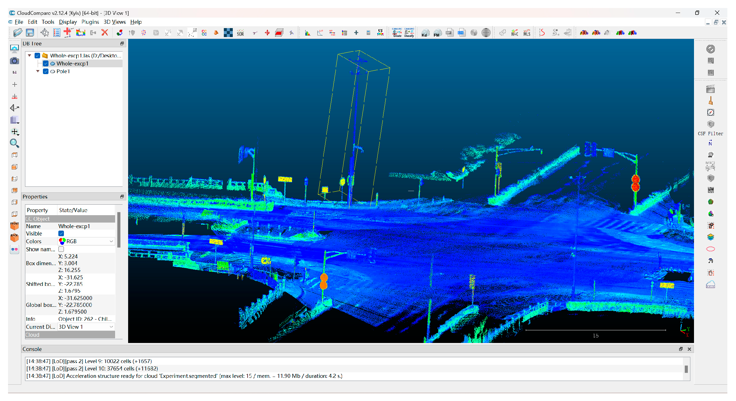
The following describes the methodology for assigning the ground truth labels to the two datasets using CloudCompare software (v2.12.4) (Figure 9):
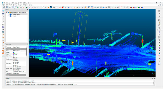
Figure 9.
Dataset annotation using CloudCompare.
- Step 1: Import the point cloud file into the software.
- Step 2: Create a scalar field associated with the point cloud and use the Edit tool to define unique class labels.
- Step 3: Manually select the points to be annotated and assign scalar values corresponding to the relevant class labels.
- Step 4: Save the annotated point clouds together with their scalar field.
3.2.2. Experimental Environment and Model Parameter Settings
The network was constructed using Python 3.8, with the experimental setup configured as follows: Windows 10 operating system, Geforce RTX 3090 TI GPU, AMD EPYC 7302 @3.0GHz CPU, CUDA 11.3, and the deep learning framework Pytorch 1.7.1.
The model was trained using the Adam optimizer, with the following parameter settings: an initial learning rate of 0.001, a learning rate decay step size of 10, a learning rate decay factor of 0.8, and a dropout keep rate of 0.5 for the fully connected layers. The KNN algorithm was set with K = 16 for neighborhood points and Knew = 10 for similar neighborhood points.
3.3. Experimental Results Analysis
3.3.1. Model Evaluation Metrics
This study employed the following main evaluation metrics for the model: accuracy per category, recall per category, F1 score, overall accuracy (OA), and average F1 score (Avg. F1), as shown in Equations (14)–(18):
where k + 1 is the number of point cloud categories, Pii represents the number of points in the dataset actually belonging to class i and predicted as class i, Pij denotes the number of points actually belonging to class i but predicted as class j, Pjj indicates the number of points actually belonging to class j and predicted as class j, and Pji represents the number of points actually belonging to class j but predicted as class i.
3.3.2. Model Results Comparison and Analysis
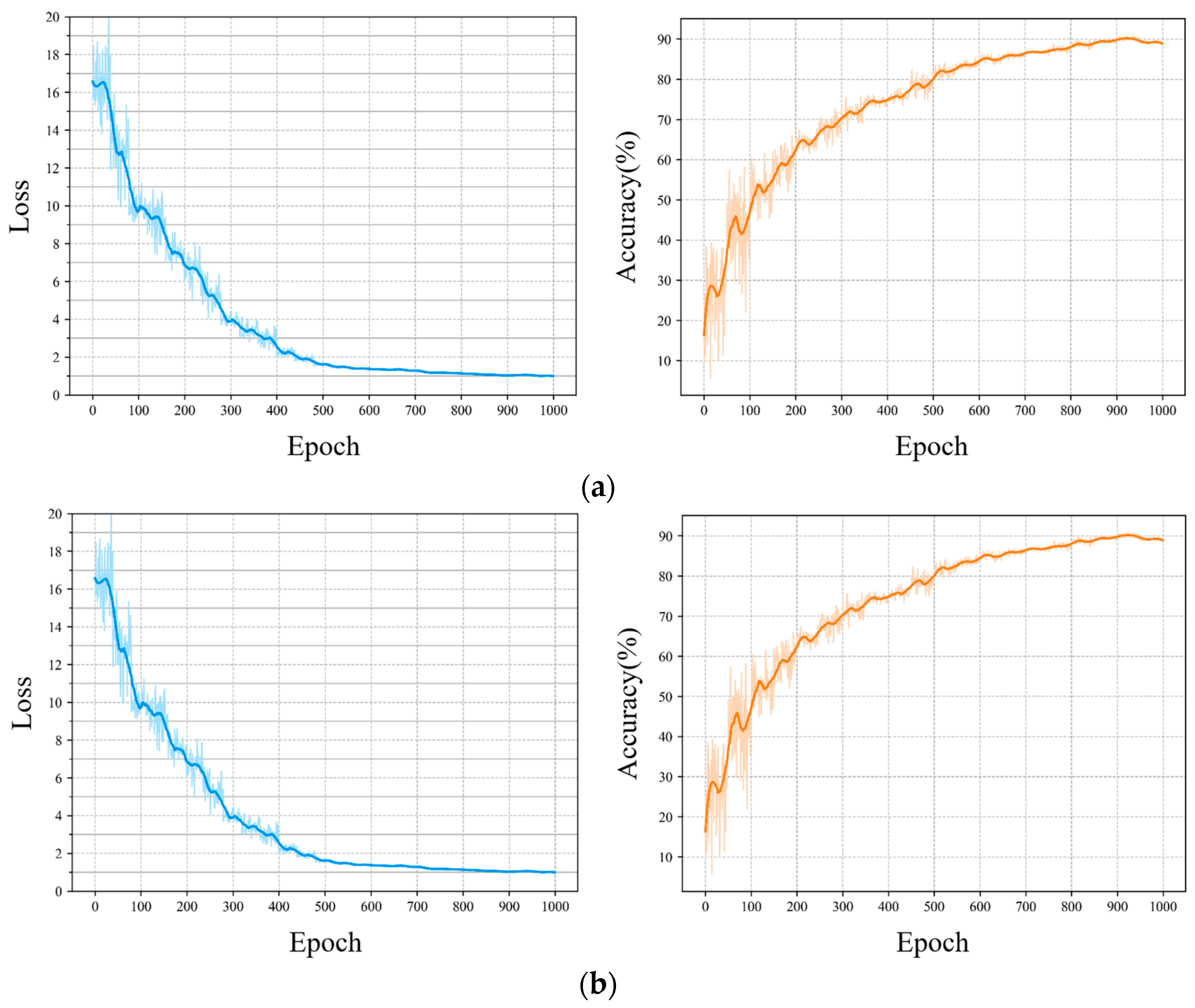
The loss function and overall accuracy curves were plotted and smoothed, as shown in Figure 10, which indicates that the loss function value gradually converged over the training process and eventually stabilized. In addition, the improvement in the segmentation performance of the model is consistent with the convergence of the loss function.
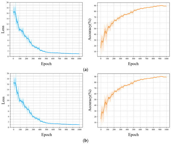
Figure 10.
Loss function and overall accuracy curves of the improved RandLA-Net. (a) Test Set 1. (b) Test Set 2.
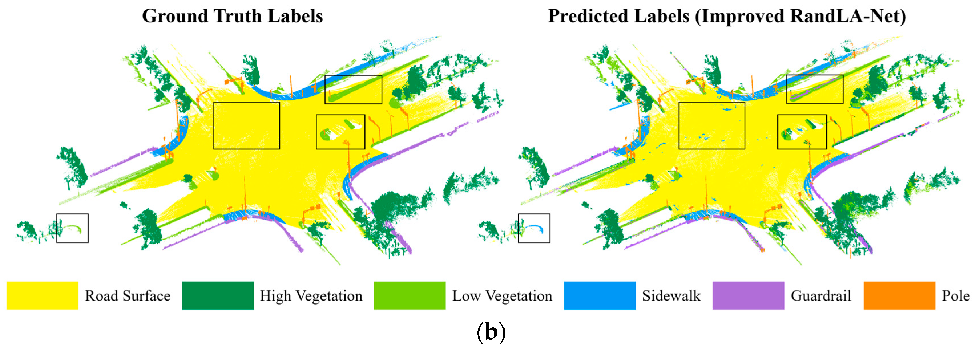
We directly analyzed the learning performance improvements under this model by comparing the output with manually annotated categories and visualizing the results, as shown in Figure 11. The semantic segmentation results of the improved RandLA-Net on the same test sets were compared with those of PointNet++ and the original RandLA-Net, as shown in Table 4 and Table 5.
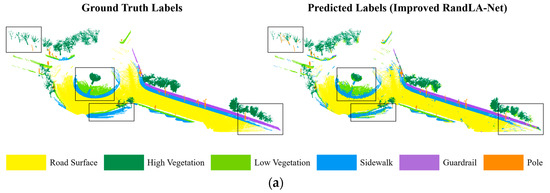

Figure 11.
Visual segmentation results for the road plane intersection point cloud. (a) Dataset 1. (b) Dataset 2.
Table 4.
Semantic segmentation results for the planar intersection point cloud (Test Set 1).
Table 5.
Semantic segmentation results for the planar intersection point cloud (Test Set 2).
4. Discussion
The results indicate that the improved RandLA-Net significantly outperformed the other two networks in terms of its overall segmentation performance. The overall prediction accuracy on the two test sets was 87.68% and 89.61%, respectively, representing an improvement of 2.40% and 2.85% over the original network. The average F1 scores were 80.61% and 82.76%, respectively, indicating improvements of 1.67% and 1.52% compared to the original network. Due to the large input sample size and distinct geometric structures of the road surface areas, their prediction F1 scores reached 95.09% and 95.63%, respectively. The recognition effects for high vegetation, guardrails, and pole-like objects were also relatively good.
The point cloud segmentation visualization results show that this method improved the ability to discriminate between different categories of point clouds. The main reason for this improvement is that the feature aggregation module excluded neighborhood points near the central sampling point with significant feature information differences, thereby preventing the network from learning redundant information. By designing the aggregation pooling layer, the point cloud’s feature expression was enriched, enabling the model to better capture the spatial structure of road scene point clouds.
In the intersection point cloud dataset used in this study, low vegetation and sidewalks had lower segmentation accuracy across all three networks due to their indistinct geometric structures and scattered distribution. Moreover, the improved network’s performance in recognizing pole-like objects did not significantly increase (with a decrease in the recall rate for this category in Test Set 1), likely because the input sample size for this category was relatively small, and the improved model’s ability to learn local feature differences and similarities was limited.
Different model architectures were designed for ablation experiments to validate the enhancement effects of the proposed improved feature aggregation module and loss function on the model’s segmentation performance, as shown in Table 6. All methods were trained on the same training and test sets, with model hyperparameter settings consistent across experiments. The results of the ablation experiments are presented in Table 7 and Table 8.
Table 6.
Ablation experiment settings.
Table 7.
Results of the ablation experiments (Test Set 1).
Table 8.
Results of the ablation experiments (Test Set 2).
The results indicate that after introducing the spatial information encoding module based on feature similarities, the model’s overall accuracy and average F1 score on the two test sets improved by 1.77%, 0.89%, 0.75%, and 0.64%, respectively. This module enhanced the network’s ability to learn neighborhood features from the input point cloud, improving the accuracy and completeness of segmentation for most categories. The use of max and average pooling functions to enhance significant local and global features of the input point cloud enabled the model to extract more spatial–structural information, thereby improving segmentation effects across all categories. Additionally, setting the weighted cross-entropy loss function improved the model’s prediction F1 scores for pole-like objects, high vegetation, and low vegetation, reflecting an improvement of the imbalanced input point cloud sample sizes.
5. Conclusions
In this study, lightweight LiDAR was utilized to collect data from typical urban road intersections. After preprocessing steps such as registration and stitching, a point cloud semantic segmentation model based on the improved RandLA-Net was applied based on the actual characteristics of road intersection scene point clouds. The main contributions of this study are as follows:
(1) Improved feature aggregation module: An improved feature aggregation module was built in addition to the original network. This module introduced a feature similarity matrix to the spatial information encoding layer, selecting neighborhood point features similar to the central sampling point’s local features as the neighborhood feature information. In the aggregation pooling layer, the results of max pooling, average pooling, and attention pooling were aggregated to extract both local neighborhood features and global information from the point cloud. To ensure a relatively balanced contribution of different category samples to the model’s loss function during training, a weighted cross-entropy loss function was also established. This loss function reduced the negative impact of uneven numbers of point clouds across categories in road scenes.
(2) Semi-automated processing framework: This study presented a semi-automated framework that integrates the use of lightweight LiDAR for data collection, point cloud registration, and semantic segmentation. This framework can extract the features of 3D point cloud data in road intersection scenarios, providing a reference for extracting operational road infrastructure information and digital asset management. Compared to RandLA-Net, this method improved the overall accuracy by 2.40% and 2.85% and the average F1 scores by 1.67% and 1.52%, respectively, for the two road intersection point cloud test sets. The segmentation accuracy was improved in each category, with the road surface area prediction accuracy reaching 94.48% and 94.79%, respectively.
However, there are some limitations in this study.
(1) Limited field data collection: Due to the limited field data collection, we trained and tested the point cloud dataset of experimental intersections only on certain effects. In the future, the improved RandLA-Net will be used to train other road intersection point clouds, further enhancing its generalization performance through model parameter adjustments and network structure optimization.
(2) Misidentification of road vegetation, sidewalks, and other facilities: The proposed semantic segmentation method misidentified road vegetation, sidewalks, and other facilities. Subsequent considerations include merging road intersection point clouds with aerial images, applying oblique photography, and using other surveying and mapping data. Introducing multi-source data features may better capture the structural information of objects in the above categories.
Author Contributions
Conceptualization, X.R. and B.Y.; methodology, X.R.; software, X.R. and Y.W.; validation, X.R. and B.Y.; formal analysis, X.R.; investigation, X.R.; resources, B.Y.; data curation, X.R. and Y.W.; writing—original draft preparation, X.R.; writing—review and editing, B.Y. and Y.W; visualization, X.R.; supervision, B.Y. and Y.W.; project administration, B.Y.; funding acquisition, B.Y. and Y.W. All authors have read and agreed to the published version of the manuscript.
Funding
This research was funded by the Natural Resources Science and Technology Program of Jiangsu Province (2023008) and the Postgraduate Research & Practice Innovation Program of Jiangsu Province (KYCX23_0294).
Institutional Review Board Statement
Not applicable.
Informed Consent Statement
Not applicable.
Data Availability Statement
Some or all data, models, and code that support the findings of this study are available from the corresponding author upon reasonable request.
Acknowledgments
This study was supported by the Natural Resources Science and Technology Program of Jiangsu Province (2023008) and the Postgraduate Research & Practice Innovation Program of Jiangsu Province (KYCX23_0294), to which the authors are very grateful.
Conflicts of Interest
The authors declare no conflicts of interest.
References
- Ma, Y.; Wang, S.; Zhang, J.; Cheng, J.; Yu, B. Automated assessment of highway vertical clearance based on vehicle-mounted LiDAR data. China J. Highw. Transp. 2022, 35, 44–59. [Google Scholar]
- Jaehoon, J.; Michael, J.; David, S.; Alireza, G.; Kamilah, B. 3D virtual intersection sight distance analysis using lidar data. Transp. Res. Part C Emerg. Technol. 2018, 86, 563–579. [Google Scholar]
- Xu, J. Road Survey and Design; China Communications Press: Beijing, China, 2016. [Google Scholar]
- Douillard, B.; Underwood, J.; Kuntz, N.; Vlaskine, V.; Quadros, A.; Morton, P.; Frenkel, A. On the segmentation of 3D LIDAR point clouds. In Proceedings of the 2011 IEEE International Conference on Robotics and Automation, Shanghai, China, 9–13 May 2011; pp. 2798–2805. [Google Scholar]
- Soilán, M.; Sánchez-Rodríguez, A.; del Río-Barral, P.; Perez-Collazo, C.; Arias, P.; Riveiro, B. Review of laser scanning technologies and their applications for road and railway infrastructure monitoring. Infrastructures 2019, 4, 58. [Google Scholar] [CrossRef]
- Yifeng, H.; Rong, H.; Jingui, Z. Analysis of point cloud segmentation algorithm for building facade using 3D laser scanning data. Surv. Mapp. Bull. 2019, 4, 26–31. [Google Scholar]
- Rastiveis, H.; Shams, A.; Sarasua, W.A.; Li, J. Automated extraction of lane markings from mobile LiDAR point clouds based on fuzzy inference. ISPRS J. Photogramm. Remote Sens. 2020, 160, 149–166. [Google Scholar]
- Fischler, M.A.; Bolles, R.C. Random sample consensus. Commun. ACM 1981, 24, 381–395. [Google Scholar] [CrossRef]
- Zhang, L.; Zhang, Y.; Chen, Z.; Xiao, P.; Luo, B. Application of split-merge based multi-model fitting method in point cloud segmentation. J. Surv. Mapp. 2018, 47, 833–843. [Google Scholar]
- Vo, A.-V.; Truong-Hong, L.; Laefer, D.F.; Bertolotto, M. Octree-based region growing for point cloud segmentation. ISPRS J. Photogramm. Remote Sens. 2015, 104, 88–100. [Google Scholar] [CrossRef]
- Yadav, M.; Singh, A.K.; Lohani, B. Computation of road geometry parameters using mobile LiDAR system. Remote Sens. Appl. Soc. Environ. 2018, 10, 18–23. [Google Scholar] [CrossRef]
- Yadav, M.; Singh, A.K.; Lohani, B. Extraction of road surface from mobile LiDAR data of complex road environment. Int. J. Remote Sens. 2020, 38, 4655–4682. [Google Scholar] [CrossRef]
- Ma, Y.; Zheng, Y.; Cheng, J.; Zhang, Y.; Han, W. A convolutional neural network method to improve efficiency and visualization in modeling driver’s visual field on roads using MLS data. Transp. Res. Part C Emerg. Technol. 2019, 106, 317–344. [Google Scholar] [CrossRef]
- Charles, R.Q.; Hao, S.; Mo, K.; Guibas, L.K. Pointnet++: Deep learning on point sets for 3d classification and segmentation. In Proceedings of the 2017 IEEE Conference on Computer Vision and Pattern Recognition (CVPR), Honolulu, HI, USA, 21–26 July 2017. [Google Scholar]
- Charles, R.Q.; Hao, S.; Mo, K.; Guibas, L.K. Pointnet++: Deep hierarchical feature learning on point sets in a metric space: Advances in neural information processing systems. In Proceedings of the 31st International Conference on Neural Information Processing Systems(NIPS 2017), Long Beach, CA, USA, 4–9 December 2017. [Google Scholar]
- Tang, L.; Zhan, Y.; Chen, Z.; Yu, B.; Tao, D. Contrastive boundary learning for point cloud segmentation. In Proceedings of the 2022 IEEE/CVF Conference on Computer Vision and Pattern Recognition (CVPR), New Orleans, LA, USA, 18–24 June 2022; pp. 8489–8499. [Google Scholar]
- Chen, Z.; Zhang, J.; Tao, D. Progressive lidar adaptation for road detection. IEEE/CAA J. Autom. Sin. 2019, 6, 693–702. [Google Scholar] [CrossRef]
- Milioto, A.; Vizzo, I.; Behley, J.; Stachniss, C. Rangenet++: Fast and accurate lidar semantic segmentation. In Proceedings of the 2019 IEEE/RSJ International Conference on Intelligent Robots and Systems (IROS), Macau, China, 3–8 November 2019; pp. 4213–4220. [Google Scholar]
- Wang, P.-S.; Liu, Y.; Guo, Y.-X.; Sun, C.-Y.; Tong, X. O-CNN: Octree-based Convolutional Neural Networks for 3D Shape Analysis. ACM Trans. Graph. 2017, 36, 72. [Google Scholar] [CrossRef]
- Han, L.; Zheng, T.; Xu, L.; Fang, L. Occuseg: Occupancy-aware 3d instance segmentation. In Proceedings of the 2020 IEEE/CVF Conference on Computer Vision and Pattern Recognition (CVPR), Seattle, WA, USA, 13–19 June 2020; pp. 2937–2946. [Google Scholar]
- Gong, J.Y.; Lou, Y.J.; Liu, F.Q.; Zhang, Z.W.; Chen, H.M.; Zhang, Z.Z.; Tan, X.; Xie, Y.; Ma, L.Z. Scene point cloud understanding and reconstruction technologies in 3D space. J. Image Graph. 2023, 28, 1741–1766. [Google Scholar]
- Han, X.; Dong, Z.; Yang, B. A point-based deep learning network for semantic segmentation of MLS point clouds. ISPRS J. Photogramm. Remote Sens. 2021, 175, 199–214. [Google Scholar] [CrossRef]
- Hu, Q.; Yang, B.; Xie, L.; Rosa, S.; Guo, Y.; Wang, Z.; Trigoni, N.; Markham, A. RandLA-net: Efficient semantic segmentation of large-scale point clouds. In Proceedings of the 2020 IEEE/CVF Conference on Computer Vision and Pattern Recognition (CVPR), Seattle, WA, USA, 13–19 June 2020; pp. 11105–11114. [Google Scholar]
- Fan, S.; Dong, Q.; Zhu, F.; Lv, Y.; Ye, P.; Wang, F.Y. SCF-Net: Learning Spatial Contextual Features for Large-Scale Point Cloud Segmentation. In Proceedings of the 2021 IEEE/CVF Conference on Computer Vision and Pattern Recognition (CVPR), Nashville, TN, USA, 20–25 June 2021; pp. 14499–14508. [Google Scholar]
- Qiu, S.; Anwar, S.; Barnes, N. Semantic Segmentation for Real Point Cloud Scenes via Bilateral Augmentation and Adaptive Fusion. In Proceedings of the 2021 IEEE/CVF Conference on Computer Vision and Pattern Recognition (CVPR), Nashville, TN, USA, 20–25 June 2021; pp. 1757–1767. [Google Scholar]
- Shuai, H.; Xu, X.; Liu, Q. Backward Attentive Fusing Network with Local Aggregation Classifier for 3D Point Cloud Semantic Segmentation. IEEE Trans. Image Process. 2021, 30, 4973–4984. [Google Scholar] [CrossRef] [PubMed]
- Li, Q.; Zhang, Y.; Fan, R.; Wang, Y.; Wang, Y.; Wang, C. MEMS mirror-based omnidirectional scanning for lidar optical systems. Opt. Lasers Eng. 2022, 158, 110–113. [Google Scholar] [CrossRef]
- Kelbe, D.; van Aardt, J.; Romanczyk, P.; van Leeuwen, M.; Cawse-Nicholson, K. Marker-free registration of forest terrestrial laser scanner data pairs with embedded confidence metrics. IEEE Trans. Geosci. Remote Sens. 2016, 54, 4314–4330. [Google Scholar] [CrossRef]
- Ren, T.; Wu, R. An acceleration algorithm of 3D point cloud registration based on iterative closet point. In Proceedings of the 2020 Asia-Pacific Conference on Image Processing, Electronics and Computers (IPEC), Dalian, China, 14–16 April 2020; pp. 271–276. [Google Scholar]
- Li, H.; Guan, H.; Lei, X.; Ma, L.; Yu, Y.; Wang, H.; Delavar, M.R.; Li, J. Urban laser point cloud classification based on point-voxel consistency constraint. China Laser 2024, 51, 1–24. [Google Scholar]
- Zhou, Z.; Huang, H.; Fang, B. Application of Weighted Cross-Entropy Loss Function in Intrusion Detection. J. Comput. Commun. 2021, 9, 1–21. [Google Scholar] [CrossRef]


Disclaimer/Publisher’s Note: The statements, opinions and data contained in all publications are solely those of the individual author(s) and contributor(s) and not of MDPI and/or the editor(s). MDPI and/or the editor(s) disclaim responsibility for any injury to people or property resulting from any ideas, methods, instructions or products referred to in the content. |
© 2024 by the authors. Licensee MDPI, Basel, Switzerland. This article is an open access article distributed under the terms and conditions of the Creative Commons Attribution (CC BY) license (https://creativecommons.org/licenses/by/4.0/).