Vector-Based Advanced Computation for Photovoltaic Devices and Arrays: Numerical Reproduction of Unusual Behaviors of Curved Photovoltaic Devices

Featured Application

It is helpful to accurately model any photovoltaic device regardless of whether a single solar cell, module (solar panel), or array of PV modules can be applied if the overall shape (including envelopes) is nonplanar, such as vehicle-integrated photovoltaics (VIPVs), agriphotovoltaics, building-integrated photovoltaics (BIPVs), aircraft PVs, and wavy PV arrays installed on wavy land (mountains, gorges, etc.).

Abstract

Most equations and models for photovoltaics are based on the assumption that photovoltaic (PV) devices are flat. Therefore, the actual performance of nonplanar PV devices should be investigated and developed. In this study, two algorithms were developed and defined using vector computations to describe a curved surface based on differential geometry and the interaction with non-uniform solar irradiance (i.e., non-uniform shading distribution in the sky). To validate the computational model, the power output from a commercial curved solar panel for the Toyota Prius 40 series was monitored at four orientation angles and in various climates. Then, these were compared with the calculation results obtained using the developed algorithm. The conventional calculation used for flat PV devices showed an overestimated performance due to ignorance of inherent errors due to curved surfaces. However, the new algorithms matched the measured trends, particularly on clear-sky days. The validated computation method for curved PV devices is advantageous for vehicle-integrated photovoltaic devices and PVs including building-integrated photovoltaics (BIPVs), drones, and agriphotovoltaics.

1. Introduction

The world is heading toward a lifestyle and industrial operational mode that rely on 100% renewable energy. After a long deliberation, we have concluded that 100% renewable energy is achievable [1,2,3,4]. One of the significant obstacles was identified in the transportation sector. Historically, most transportation fuels have been fossil fuels, and internal combustion engines (ICEs) have been used. However, advanced modeling and alternative mobility technologies have made a 100% renewable energy scenario for the transportation sector potentially viable [5,6]. Photovoltaic (PV) energy is the leading primary energy source [7]. PV charging stations were the first application considered and the one that prevailed worldwide in providing power from PVs to automobiles [8,9,10,11,12,13]. Vehicle-integrated photovoltaics (VIPVs) and car-roof PVs have been used by engineers to provide realistic and convenient modes of feeding renewable energy to automobiles. Many studies have discussed the feasibility of PV-fed transportation and revealed its potential [14,15,16,17,18,19,20,21,22,23,24,25,26,27,28]. The limitations of the car body’s geometrical area and the energy requirements have induced solar cell researchers to develop more innovative solar cells [29,30]. Specifically, various generations of solar cells were considered for application to vehicles. Due to the amount of energy yield of vehicles with a limited installation area, the power conversion efficiency of PV devices is crucial, and Yamaguchi discussed the possibilities and future development [31].

A VIPV is a rather sophisticated PV panel installed on the body or roof of a car. Several technological challenges should be addressed [14]. A few of these issues are related to the structural constraints of automobiles and require new design considerations. Many new developments have been made, such as lightweight, robust, flexible, and curved surfaces for both car bodies and VIPVs [32,33,34,35,36,37,38,39,40,41,42,43,44,45,46,47,48,49,50,51,52,53,54,55,56]. Recently, Toyota Motors developed a lightweight plastic-covered VIPV with sufficient strength as the exterior of a car [57].

In addition to these mechanical issues, the VIPV should enclose the curved surface of the car body. In general, PV panels are flat and not designed to enclose curved surfaces. Therefore, covering curved surfaces causes problems such as mechanical stress and mismatching losses [58,59,60]. Several innovative PVs suitable for enclosing curved surfaces have been developed recently [61,62]. VIPVs were evaluated recently, including the curved surface and impact from temperature [63,64]. In addition, our group proposed correcting the curved surface effect using a unique curve correction factor [65,66,67]. The shape of the curved surface varies significantly according to the automobile product line. This impacts the power generation performance and durability [68]. For a general discussion on VIPVs, it is necessary to understand the various curve shapes and general rules that affect the optical, thermal, and mechanical properties of PV panels based on global and local differences. Quantitatively comprehending the quantity and type of curved surface an actual automobile body has would help in developing versatile VIPV technology and measurement protocols [69]. It would also be effective for quantifying the advantages of VIPVs, such as the stability of the energy source for various VIPVs with various curved surface shapes during actual driving and the decrease in the frequency of charge replenishment [70,71].

PV technologies rely on the assumption that all solar panels have flat surfaces. Many PV-related equations are implicitly based on this assumption. The curved PVs necessary for VIPVs override this assumption. We need to identify a new technology. Our approach uses a vector-based computation of curved PV modules from a flat PV framework. Furthermore, it is effective in helping us to understand the general behavior of PV devices resulting from the curved surface of vehicle bodies by evaluating modeling algorithms. It is necessary to examine measurement protocols that are not biased against the diversity of curved surfaces, apply various curved surface models to evaluate the measurement method, and perform numerical experiments for verification. The geometric condition of the curved surfaces should express the optical properties of the PV module and the mismatching loss [72,73,74,75,76,77,78].

The curved surface of PVs is also related to mechanical and geometrical issues (increasing and optimizing the packing density) [14,62,69,71,79,80,81,82,83,84,85,86,87,88,89,90,91,92,93]. The curved surface, generally a 3D curved surface (undevelopable), commonly seen in vehicle bodies cannot be covered by a flat plane. Namely, it cannot be covered by the flexible types of photovoltaic devices without generating wrinkles. Typically, it is covered only in the relatively flat zone of the vehicle bodies, leading to a reduced coverage of the curved surface and thus reducing the amount of power. The typical coverage ratio of a photovoltaic device in the entire roof area of a vehicle is 70%. Such a low coverage ratio is as significant as the power conversion efficiency. These factors need to be solved as a mechanical constraint optimization problem, which this study did not investigate.

This article begins by describing a curved surface, aided by differential geometry. Then, we expand it to the interaction with non-uniform solar irradiance that is observed frequently in vehicles running in the valleys of buildings. For this purpose, we define a four-tensor (nested matrix) to characterize the interaction. Reducing the complexity of certain applications, such as PV devices on car roofs, is feasible. First, we do not need to consider the 3D rotation of the coordinate system (pitch, roll, and yaw); we only need to consider the vehicle’s orientation. Second, the curve shape is simple convex (single peak), and we do not need to consider the hidden surface; thus, we only consider the inner product of the normal vector of the surface element and the ray vector. Third, solar cells are connected in series (single string configuration). In such cases, the calculation steps are not complex. Still, it is beyond arithmetic with trigonometric functions. The new algorithm for curved PV devices was validated using a commercial VIPV panel. It effectively explains the performance of PV modules in an outdoor environment with dramatic differences between standard and flat PV devices.

The unusual behavior of curved PV devices in VIPV applications has been intensively considered and analyzed. Therefore, the modeling, measurement, analysis, and discussions of curved issues were focused on VIPVs in this study. However, they can also be applied to curved PV devices such as building-integrated photovoltaics (BIPVs), aircraft PVs, and even PV arrays installed on wavy land.

2. Methods

2.1. Impact of the Curved Surface

All the formulas and protocols for measuring the performance of PV modules are based on the precondition that the PV modules are flat. For example, it is essential to determine the output power and other fundamental electrical parameters such as the short-circuit current (Isc), open-circuit voltage (Voc), and fill factor (FF). The aperture area of the curved PV device differs from the surface of the module. The vehicle roof is curved three-dimensionally. Its curvature can induce power loss through cosine and self-shading losses. The orientation of the VIPV varies with time without any correlation with the orientation of the sun. These factors have different effects on a curved shape. These interactions also need to be considered.

The efficiency of curved modules is generally overestimated [68]. Solar simulators frequently underestimate the input energy. The aperture area of a standard flat PV device is equal to the active area of the module. However, this area is not on a curved surface because the aperture area is defined as the window of the flat plane.

First, a curved PV module generally collects more light than an aperture window. As the solar simulator illuminates a larger area than the PV module, a curved module receives more unexpected light from the outer region to generate more unexpected power, because the aperture area and the area of the active area of curved PV devices are different (the active area is more substantial than the aperture area). However, they are the same for flat PV devices. Placing an aperture mask on a curved PV module is a highly effective alternative.

The second reason is the aperture area. The area of the active zone of the curved PV device is not clearly defined.

The third cause is the angular distribution difference between indoor and outdoor VIPV operations. Depending on the points on the surface, curved PV devices induce larger illumination losses at higher incident angles. Unlike flat PV modules, this approach cannot be applied to improve the efficiency of indoor modules in outdoor operations. It is essential to correct the curved shape.

Also, this study covered a surface containing a flat zone in the curved surface or an entire flat plane. Based on differential geometry, the equations used in this study cover flat planes, which is the particular case for the curved surface. Note that the input is the X, Y, and Z coordinates, and we did not use equations that potentially lead to division by zero.

2.2. Impact of the Non-Uniform Solar Irradiance

Building-integrated photovoltaics (BIPVs) and vehicle-integrated photovoltaics (VIPVs) receive solar irradiance through non-uniform shading objects. Standard scalar calculations cannot accurately determine the solar irradiance of BIPV and VIPV systems. This study proposes a matrix model using an aperture matrix to accurately calculate the horizontal and vertical planes affected by non-uniform shading objects. Applying a local coordinate system can extend this to the solar irradiance on a VIPV. Fish-eye videos were used to measure the non-uniform solar irradiance of the vehicle’s surroundings. With the help of image processing calculations, the shaded objects and sky were discriminated using the binarizing algorithm [71]. The 3D model was validated by simultaneously measuring five orientations (roof and four sides: front, left, tail, and right) of solar irradiance on a car body [71].

The shaded objects distributed around the VIPV are essential for performance. The aperture matrix E was defined using a 2D histogram of the angular distribution of the shaded objects. The matrix elements are real numbers ranging from zero to one (zero: shaded; one: unshaded). Shading refers to the shading of a 2D bin in a hemispherical sky. The (i, j) elements, E_i,j, are the probabilities of the unshaded 2D bin of the elevation angles [i°, (i + 1)°] (i = 0, 1, …. 89) and orientation angles [4j°, 4(j + 1)°] (j = 0, 1, …, 89) (Scheme 1) [69,70,71]:

The solar irradiances from the direct and diffused components were calculated independently using the aperture matrix, which weighs and discriminates between shading and the contribution of diffuse sunlight from the sky. The measured solar irradiance matched the calculated values regardless of the shading environment (open zone, residential zone, and building zone), orientation of the solar panels, and position of the sun [71]. For energy yield estimation, the matrix may be replaced with probability curves to estimate the energy as the expected value of the power variations by probability [71].

2.3. Interaction between Curved Surfaces and Non-Uniform Solar Irradiance

A typical PV calculation assumes a uniform, hemispherical sky with no shadows. However, a VIPV receives non-uniform and frequent shadows with partial and dynamic shading. The classic and well-acknowledged solar calculation is arithmetic with trigonometric functions such as sine, cosine, and tangent. Classical calculations use absolute ground coordinates. However, the new analysis uses a local coordinate system with 3D rotation. The proposed approach uses vector computation.

Such computation requires a shading (aperture) matrix, instead of a shading ratio or angle (scalar), a tensor form (4-tensor) for the angular response to the incident light instead of the Lambertian curve, and differential geometry description using the vector expression of a unit element, instead of cosine loss due to the angles of the PV panel (

Table 1. Comparison of the differences between vehicle applications and typical PV devices.

	Typical PV Devices	Vehicle Applications
Shape of PV devices (cells and modules)	Flat surface	Curved surface (undevelopable curved surface) based on differential geometry
Basic math	Arithmetic with trigonometric functions	Vector computations
Ray orientation	Cosine	The inner product between the normal vector of the surface element and rays
Angular response	Lambertian	4-tensor
Coordinate system	Absolute ground coordinates	Local coordinates with 3D rotation
Sky model	Uniform hemisphere sky (Shading ratio: scalar)	Non-uniform shading on hemisphere sky (Shading matrix: matrix)
Partial and dynamic shading 1	Time integration with weighting	Statistical model on probabilities and expected values
Stress calculation1	Bending load to a thin plate	Buckling by 3D bending owing to coverage of an undevelopable curved surface (differential geometry and continuum dynamics)

¹ Not performed in this article.

). The coordinate system may also shift to a local coordinate system with 3D rotation rather than absolute ground coordinates.

Although advanced calculations and modeling can explain the unusual behavior of VIPVs, the rating method is challenging to assess because of its transparency requirements. That is, everyone can calculate and attain an equal value. An approximation with a clear formulation is required for a simple arithmetic calculation. However, this was not addressed in the present study.

Many vehicles have curved roofs, and typical VIPVs have curved surfaces. However, curved PVs typically perform less efficiently than flat PVs because of two factors. First, the aperture area of a curved surface is smaller than that of a flat surface. The input power to the PV devices is the product of the aperture area and irradiance. Therefore, the smaller the aperture of the curved PV devices, the less the input power that these devices receive. Another factor is that the cosine loss of a curved surface varies at different points, thereby generating a mismatch loss.

There are two degrees of freedom in the 3D space direction, and two indices can describe the surface. The 2 × 2 combination generates a nested matrix or four-tensor, as described by Equations (1) and (2) [71]:

$$\mathit{M}\mathit{M}=\left[\begin{array}{ccccccc}{\mathit{M}}_{0,0}& {\mathit{M}}_{0,1}& {\mathit{M}}_{0,2}& & {\mathit{M}}_{0,l}& & {\mathit{M}}_{0,NN-1}\\ {\mathit{M}}_{1,0}& {\mathit{M}}_{1,1}& {\mathit{M}}_{1,2}& \cdots & {\mathit{M}}_{1,l}& \cdots & {\mathit{M}}_{1,NN-1}\\ {\mathit{M}}_{2,0}& {\mathit{M}}_{2,1}& {\mathit{M}}_{2,2}& & {\mathit{M}}_{2,l}& & {\mathit{M}}_{2,NN-1}\\ ⋮& ⋮& ⋮& \ddots & & & \\ {\mathit{M}}_{k,0}& {\mathit{M}}_{k,1}& {\mathit{M}}_{k,2}& & {\mathit{M}}_{k,l}& \cdots & {\mathit{M}}_{k,NN-1}\\ ⋮& ⋮& ⋮& \cdots & ⋮& \ddots & ⋮\\ {\mathit{M}}_{NN-1,0}& {\mathit{M}}_{NN-1,1}& {\mathit{M}}_{NN-1,2}& & {\mathit{M}}_{NN-1,l}& \cdots & {\mathit{M}}_{NN-1,NN-1}\end{array}\right]$$

(1)

$${\mathit{M}}_{k,l}=\left[\begin{array}{ccccccc}{\mathit{m}}_{0,0}& {\mathit{m}}_{0,1}& {\mathit{m}}_{0,2}& & {\mathit{m}}_{0,j}& & {\mathit{m}}_{0,N-1}\\ {\mathit{m}}_{1,0}& {\mathit{m}}_{1,1}& {\mathit{m}}_{1,2}& \cdots & {\mathit{m}}_{1,j}& \cdots & {\mathit{m}}_{1,N-1}\\ {\mathit{m}}_{2,0}& {\mathit{m}}_{2,1}& {\mathit{m}}_{2,2}& & {\mathit{m}}_{2,j}& & {\mathit{m}}_{2,N-1}\\ ⋮& ⋮& ⋮& \ddots & & & \\ {\mathit{m}}_{i,0}& {\mathit{m}}_{i,1}& {\mathit{m}}_{i,2}& & {\mathit{m}}_{i,j}& \cdots & {\mathit{m}}_{i,N-1}\\ ⋮& ⋮& ⋮& \cdots & ⋮& \ddots & ⋮\\ {\mathit{m}}_{N-1,0}& {\mathit{m}}_{N-1,1}& {\mathit{m}}_{N-1,2}& & {\mathit{m}}_{N-1,j}& \cdots & {\mathit{m}}_{N-1,N-1}\end{array}\right]$$

(2)

The four-tensor MM has a nested matrix element M. M_k,l are matrices with m_i,j scalar elements. The matrix m is the 2D angular response of the surface elements positioned at (k,l).

In general, the four-tensor has a substantial number of elements. If both matrix MM in Equation (1) and M in Equation (2) are 100 × 100, the total number of elements would be 100⁴ = 100,000,000. Therefore, it is ineffective to recalculate or regenerate the four-tensor each time the position of the sun or orientation of the vehicle varies. Alternatively, the four-tensor is calculated immediately, and each deviation from the angles from the reference four-tensor is calculated by 2D interpolation such as bicubic interpolation (2D spline interpolation) (Figure 1). The movement of the sun and PV devices is considered as a rotational transformation of the four-tensor.

2.4. Expression of Curved Surfaces of PVs

In a curved PV, the shade owing to self-shadowing and cosine loss differs depending on the panel’s PV location. Therefore, each cell is not irradiated with uniform sunlight. That is, the total amount of solar radiation and the amount of solar radiation absorbed by the PV system do not match. Moreover, the degree of solar radiation varies in a complex manner depending on the curved surface shape, orientation of the automobile, sun, and distribution of the surrounding structures. Through this research, we formulated a method for determining the distribution of cosine loss, self-shadow, direction vector of face elements, and area of surface elements at each curved surface. We also developed a method for determining the distribution of cosine loss, self-shadow, direction vector of surface elements, and surface elements’ area at each curved surface. For example, if a 3D measurement result exists for the shape of the car body roof, it is also feasible to calculate the solar radiation distribution in each part.

The non-uniform distribution of solar radiation intensity on the curved surface induces a mismatch loss in the module. This mismatch loss is a significant loss factor in VIPVs. Symptomatic treatments such as mounting multiple MPPTs and developing string configurations are known to cause mismatch losses. For a quantitative analysis of the mismatching phenomena and design optimization, each solar cell that comprises the module should determine the amount of incident light. Therefore, it is essential to calculate the short-circuit current of each cell by dividing the area of sunlight irradiating the surface integral in each cell region and calculating various quantities based on the curved surface geometry.

Each face surface element, normal vector, and first derivative in each direction are required. The parametric format shown in Equation (3) is convenient:

$$\mathit{S}(u,v)=\left[\begin{array}{c}\mathit{x}(u,v)\\ \mathit{y}(u,v)\\ \mathit{z}(u,v)\end{array}\right],$$

(3)

The uv plane is a matrix in which grid-point position information is arranged. The actual curved surface exists in the XYZ space, and Equation (3) represents the mapping from the uv plane to the XYZ space. It is an image of a square rubber film on a flat surface that is stretched or twisted and placed in a 3D space.

The grid points do not need to be squares. It is necessary to make these non-uniform and rectangular because the approximation would be higher if the grid points are set finer in the region where the curve is steep. Therefore, as shown in Equation (3), it is necessary to expand the mapping target in the z-direction profile and the x and y directions.

The derivative was calculated using numerical differentiation based on the central difference, as shown in Equations (4) and (5):

$${{\mathit{S}}_{\mathbf{u}}}_{i,j}=\left[\begin{array}{c}{{\mathbf{S}}_0}_{i,j}-{{\mathbf{S}}_0}_{i+2,j}\\ {{\mathbf{S}}_1}_{i,j}-{{\mathbf{S}}_1}_{i+2,j}\\ {{\mathbf{S}}_2}_{i,j}-{{\mathbf{S}}_2}_{i+2,j}\end{array}\right]$$

(4)

$${{\mathit{S}}_{\mathbf{v}}}_{i,j}=\left[\begin{array}{c}{{\mathbf{S}}_0}_{i,j}-{{\mathbf{S}}_0}_{i,j+2}\\ {{\mathbf{S}}_1}_{i,j}-{{\mathbf{S}}_1}_{i,j+2}\\ {{\mathbf{S}}_2}_{i,j}-{{\mathbf{S}}_2}_{i,j+2}\end{array}\right]$$

(5)

The S_u and S_v 3 × 1 vectors nest a matrix with rows and columns corresponding to the number of lattice points as elements. These display the partial differentials in the u and v directions in the parameter space (uv plane). In addition, S represents the curved surface coordinates in the XYZ space. The values of x, y, and z in the subscripts (row number, column number) i and j corresponding to the lattice points in the uv plane are stored as a matrix. It is a 3 × 1 vector element. That is, the first, second, and third lines (lines 0, 1, and 2, respectively) store the x, y, and z coordinates, respectively.

To calculate the VIPV efficiency, the surface area of the curved surface needs to be calculated. This can be obtained by integrating the plane elements.

Equations (6) and (7) can be used to calculate the area of the surface element and normal vector:

$${\mathit{s}}_{i,j}=\left|{{\mathbf{S}}_{\mathit{u}}}_{i,j}\times {{\mathbf{S}}_{\mathit{v}}}_{i,j}\right|$$

(6)

$${\mathit{n}}_{i,j}=\frac{{{\mathbf{S}}_{\mathit{u}}}_{i,j}\times {{\mathbf{S}}_{\mathit{v}}}_{i,j}}{\left|{{\mathbf{S}}_{\mathit{u}}}_{i,j}\times {{\mathbf{S}}_{\mathit{v}}}_{i,j}\right|}$$

(7)

where s and n are matrices with the face element area and normal vector, respectively. Because S_u and S_v are vectors, the operator × representing the product indicates the operation of the outer product.

When calculating the cosine loss, the inner product of the normal vector of each surface element and the ray direction vector can be integrated using Equations (8)–(10): the self-shadow can be determined by the signs of the normal vector and the ray’s inner product unless it is an exceptional vehicle body with a valley, such as a double bubble or saddle-curved body. A face element with an inner product of at most zero can be regarded as not being hit by a light beam owing to its own shadow. Specifically, the following formula can be converted into logical values:

$${\mathit{n}\mathit{n}}_k=\left[\begin{array}{c}\mathrm{s}\mathrm{i}\mathrm{n}\left({\mathit{\varphi }}_k\right)·\mathrm{s}\mathrm{i}\mathrm{n}\left({\mathit{\theta }}_k\right)\\ \mathrm{c}\mathrm{o}\mathrm{s}\left({\mathit{\varphi }}_k\right)·\mathrm{s}\mathrm{i}\mathrm{n}\left({\mathit{\theta }}_k\right)\\ \mathrm{c}\mathrm{o}\mathrm{s}\left({\mathit{\theta }}_k\right)\end{array}\right]$$

(8)

$${{\mathit{S}\mathit{C}}_{i,j}}_k={\mathit{n}}_{i,j}·{\mathit{n}\mathit{n}}_k$$

(9)

$${{\mathit{S}\mathit{S}}_{i,j}}_k=\left({\mathit{n}}_{i,j}·{\mathit{n}\mathit{n}}_k>0\right)$$

(10)

nn_k is a 3 × 1 vector of the ray’s direction to the PV with an incident angle θ_k and directional angle ϕ_k. Uniformly distributed random numbers provide angles ranging from 0° to 90° for θ_k and from 0° to 360° for ϕ_k. The index number k identifies each set of random numbers ranging from 0 to 999,999. According to our experience, the total number of rays required to be a repeatable result, 1,000,000, is frequently used for ray-tracing simulations. Our calculation follows this rule. SC and SS are vectors whose elements are matrices that store the local cosines and logical values of the presence or absence of a self-shadow. Each element becomes a self-shadowing distribution matrix corresponding to k sunlight ray vectors. A point without self-shadowing stores one (TRUE) and a point with self-shadowing stores zero (FALSE). The dot operator indicates the inner product of the vectors. Because VIPVs are affected by the relative position of the sun and by light scattered and reflected from the road surface, it is necessary to consider all these and perform weighted integration according to the angular distribution of light rays. When identifying a long-term angular distribution such as the annual power generation, the vehicle’s orientation can be regarded as a random distribution that follows a uniform distribution uncorrelated with the sun’s direction. Therefore, it is feasible to approximate using only the sun’s altitude. The number of rows and columns of the normal vector of the plane element is less than that of the original grid points because the central difference is used.

When performing ray tracing, it is necessary to program a detector model whose shape matches that of the curved surface [94,95,96]. The light source model should be generated by programming the angle distribution of solar radiation on the vehicle surface (shadow and wall reflection by the structures around the street and reflected light from the road surface) in different regions [97]. For example, when measuring a curved surface using a coordinate measurement machine (CMM), interpolation techniques are required (typically using cubic polynomials) [98,99,100].

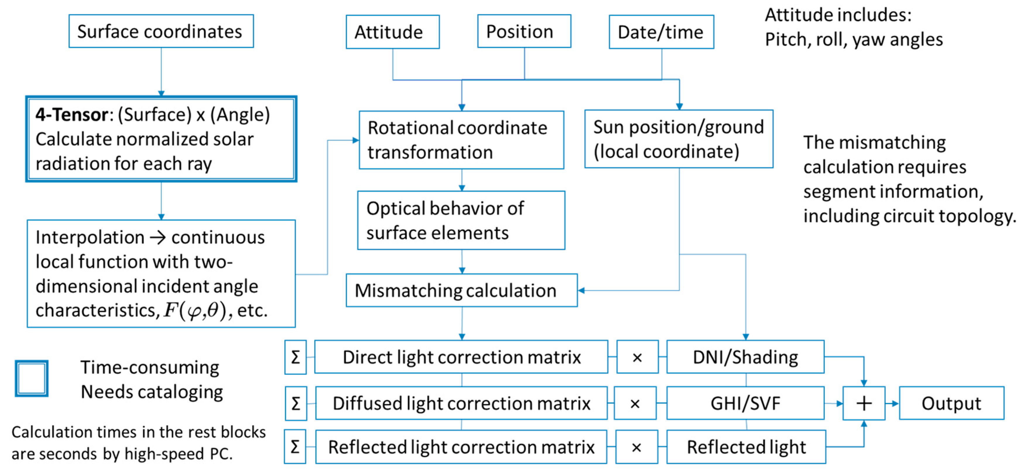
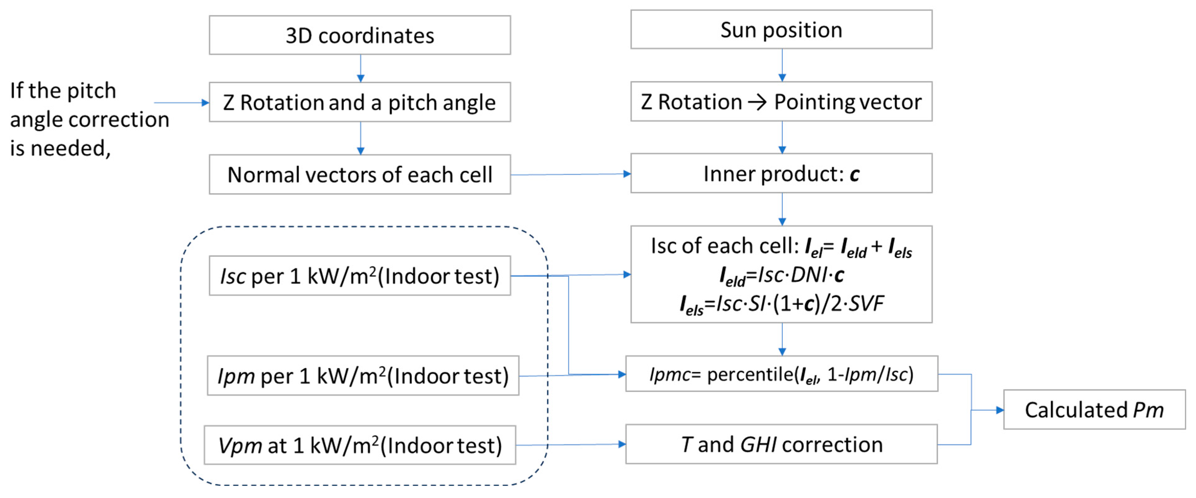
2.5. Simplified Calculation for VIPVs or Other Loosely Curved PV Devices

A simplified flowchart of the computation for the PV module on a car roof is shown in Figure 2. It can be used under the following conditions:

• The attitude and position remain constant during the timeframe of the power measurement.
• The solar irradiance angular distribution remains constant during the power measurement timeframe.
• The surface is a simple concave shape (not saddle-shaped or with multiple peaks, such as a twin bubble roof) [101,102].
• All the solar cells are connected in series.
• The nonlinear effects in the equivalent circuits in solar cells are negligible [103,104].
• The spectrum mismatching loss is negligible [105,106,107].
• The dynamic and partial shadings are negligible [108,109,110].

The stress calculation substantially impacts the mechanical robustness (cell crack) and reliability (impact strength, vibration, and fatigue degradation) but does not significantly impact the initial performance unless it is heavily deflected, leading to the cell cracking [14].

The impact of dynamic and partial shading varies dramatically depending on the relative position of shading objects and the sun, as well as the vehicle’s orientation. Several publications have quantitatively analyzed these impacts [108,109,110].

The percentile function (v,p) in Figure 2 returns a value below which p percent of the data are recorded in v (vector). Iel in Figure 2 represents the vector data of the Isc of each cell; Ield in Figure 2 corresponds to the Isc of each cell generated by direct solar irradiance; and Iels represents that of diffused sunlight. The vector or matrix c is the inner product of the normal vector of the cell and the ray vector (the directional vector of direct sunlight). This is calculated using the areal integration of Equations (9) and (10) for the entire area of each solar cell divided by the total area of the cell calculated by the sum or integration in Equation (6).

In this situation, the time-saving advantage of computing using a four-tensor, similar to the one in Figure 1, is not apparent. The detection of the hidden surface generally observed in saddle-shaped aircraft wings and double-bubble roofs in superior aerodynamic vehicles (which requires a considerable amount of computation) is not required. Equations (9) and (10) are used to calculate the entire angular response without hidden surfaces in any surface element. These are simple inner products of vectors, and their nonzero discrimination and computation time are moderate. Therefore, we can directly apply Equations (9) and (10) without interpolating the four-tensor described in Figure 1.

Computing the power output from each cell by considering the angular response is not necessary. Rather, a single solar cell with a specific percentile value of the order of the cosine value to the ray vector of direct sunlight is used to determine the total power output from the module. Unless the mismatch loss is large (which causes the maximum power point peak to shift to another value and occurs frequently in the case of partial or dynamic shading), the overall shape of the I-V curve does not vary dramatically. Moreover, the solar cell that controls the position of the maximum power point remains unaltered. This study did not solve differential or partial differential equations, numerically or analytically, but relied on the calculation of geometries (differential geometry). Although we frequently used tensor, matrix, and vector computations, we were not required to define boundary conditions.

In certain cases, the indoor test is performed on the test bed in testing laboratories. It has a different angle of placement relative to the ground on the actual car roof. In such cases, the group of normal vectors of the surface element is transformed by coordinate rotation by applying rotation matrices.

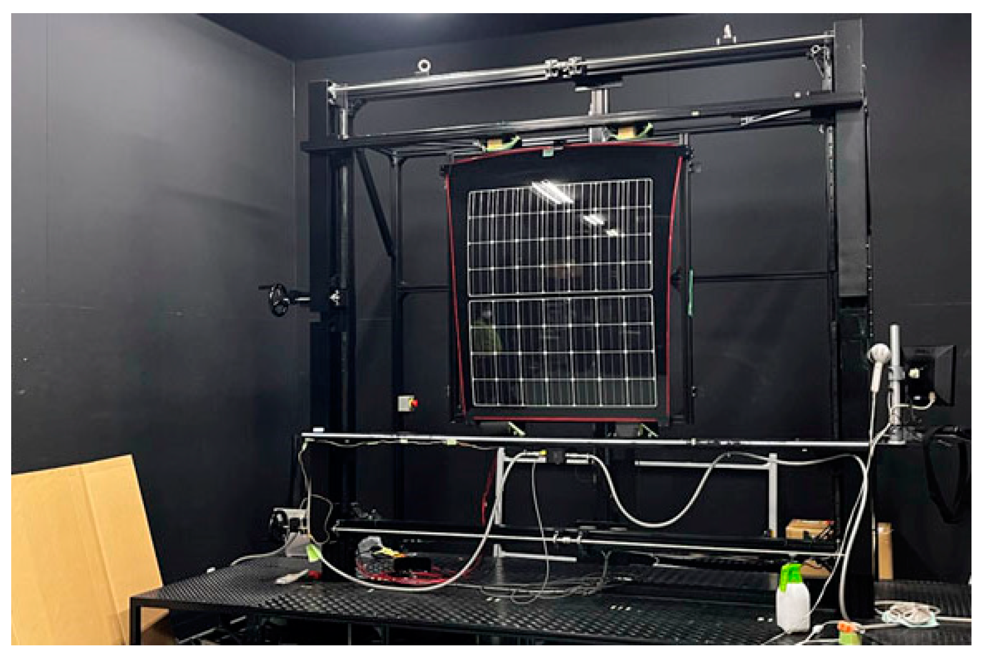
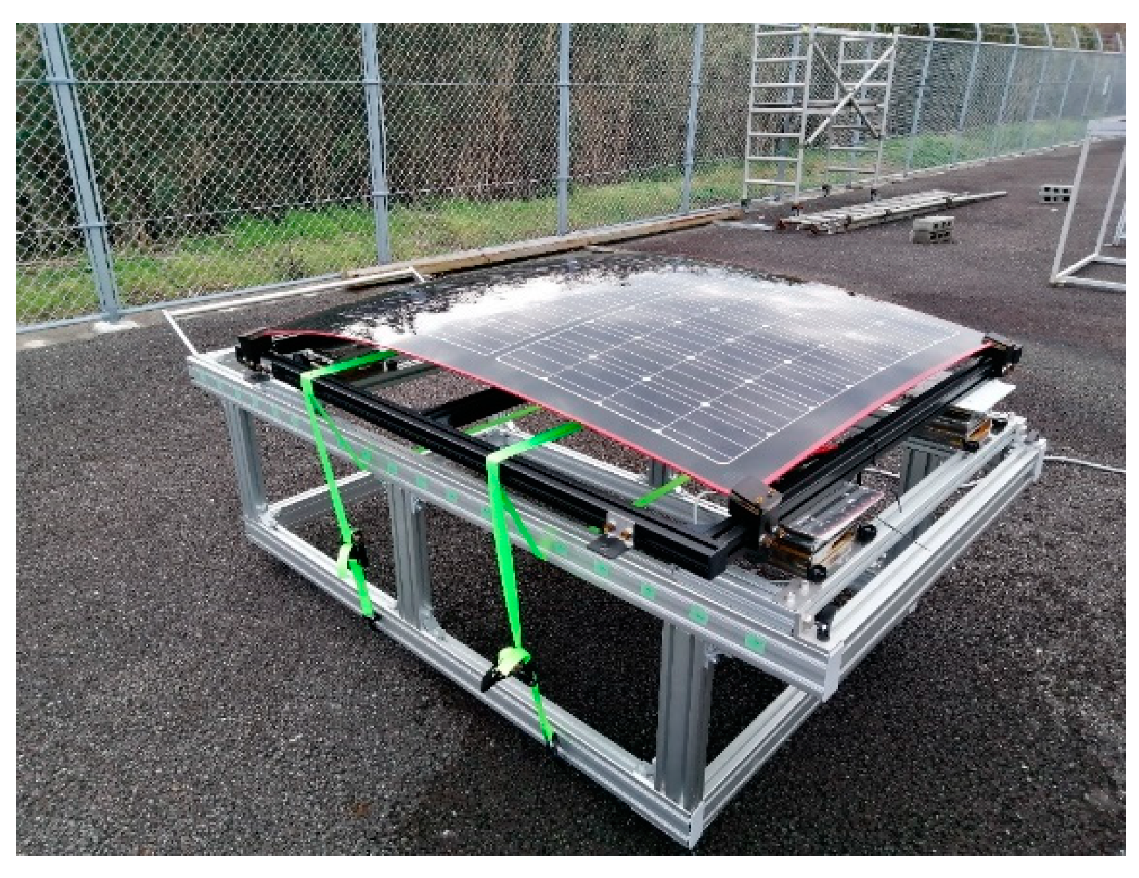
2.6. Curve-Shape Measurements and Indoor Tests

To identify the unusual behavior of the curved PV modules and validate the computational model, we conducted a series of measurements using a commercial curved PV module and the solar roof of the Toyota Prius 40 series (Toyota, Japan).

Because the optical and performance characteristics of the curved module are sensitive to angle errors and because we considered it essential to set the module at equal angles, we prepared a module carrier (holding fixture). The module was set throughout the manufacturing process, storage, and transportation (Figure 3). Curved PV devices should be held on a stable contact plane to prevent deflection, gravity distortion, and stress from the holders. The holding fixture did not shade the solar cells in the module.

The frame was attached externally to prevent deflection and deformation of the curved PV devices and damage caused by dropping or handling. An example is shown in Figure 3. The frame should satisfy the following conditions for holding curved PV modules:

• The reference bottom surface (bracket or frame bottom surface) is flat across the bottom. As a criterion for assessment, it should be placed on a surface plate that is larger than the frame, and a force should be applied to at least three corners to ensure adequate tightness. The permissible deflection is 10 mm using a 100 N load force.
• The frame, bracket, and enveloping holder surfaces are outside the envelope surface of the module outline.
• At least three holders are provided to hold the modules.
• The holder’s height is lower than that of the neighboring cells.
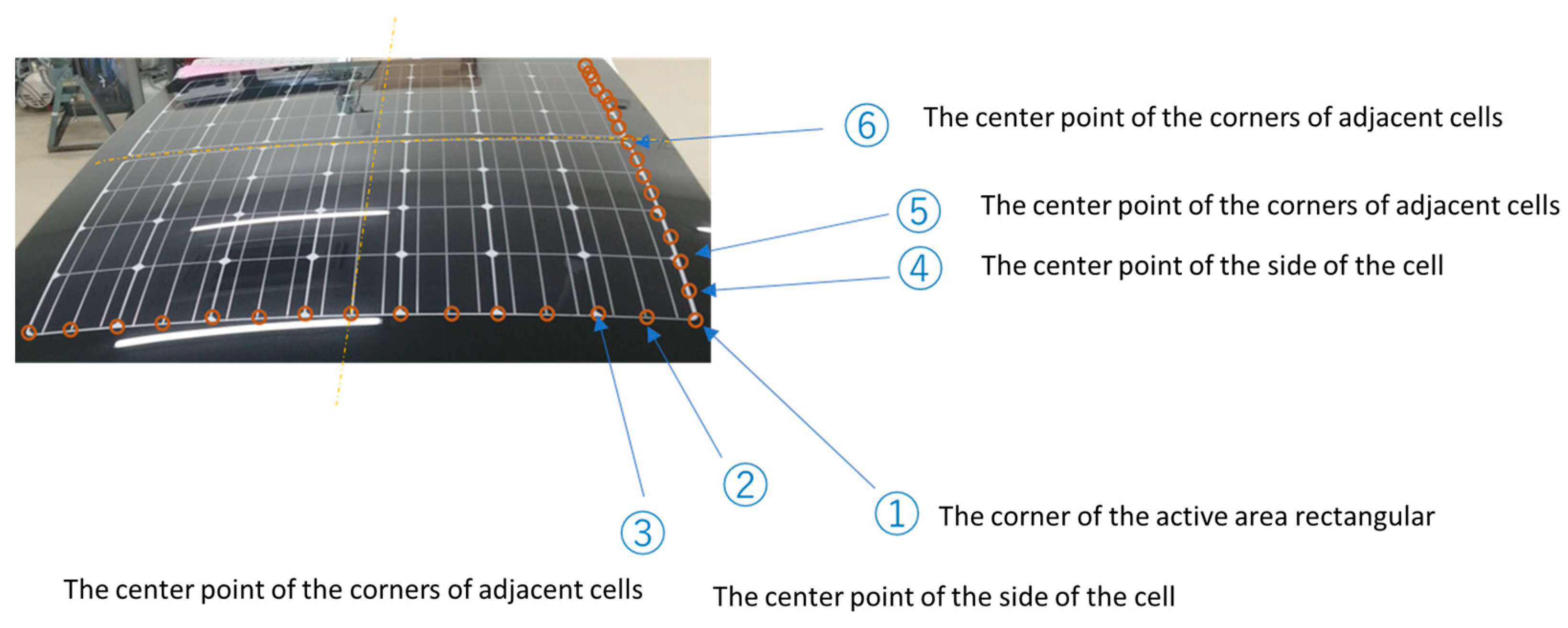
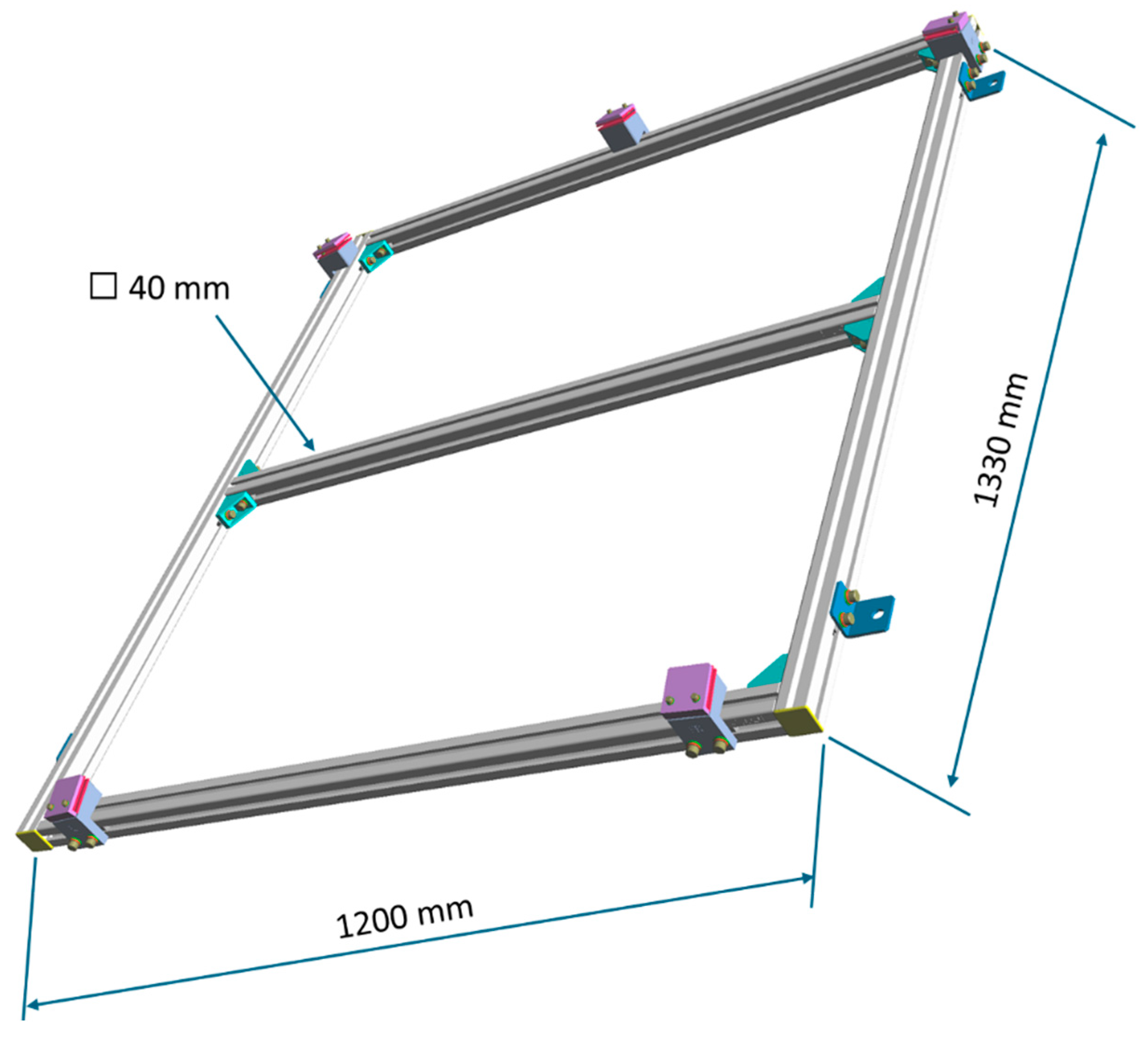
• To prevent module deformation (twisting) during fastening, all the holders have an angle-adjustment function to follow the variations in the curved surface shape (purple plates on the four corners and a center point of a side in Figure 3).
• The central tilt angle for the angle adjustment of the holder (Figure 3) is designed based on the aspects of the module. Specifically, the module is placed on a horizontal surface plate (there is no need to compensate for deflection owing to its weight). The angle of inclination of the edge of the module at the point where it is fixed with a holder is measured using a protractor or a small inclinometer. The center angle of the holder (14° in Figure 3) is determined according to the estimated value.
• To prevent the glass cover from cracking during fastening, the fastening part is sandwiched between 3 mm thick urethane plates. Furthermore, the fastening torque is controlled (e.g., 2-M4 fastening torque of 1 Nm).
• The surface viewed from the light-receiving surface is matte black in color. Any surface treatment method such as black alumite treatment, black dyeing, black chromate treatment, black nickel plating, or matte painting can be used. The surfaces concealed behind the module are not black. Non-black surfaces such as screw heads and machined surfaces may remain if these are negligible in terms of the projected area of the frame.
• The module is attached to a rail for convenience. For example, in a series of set operations such as removing the upper holding portion of the holder, placing the module, adjusting the position, and tightening the upper holding portion, the module does not slip or need to be held temporarily.
• Specifically, the frame is placed on the surface plate, the top is removed, a part of the holder is pressed, the module is enabled to stand, and the distance from the plate surface to the lower end of the module (mechanical contact plane) is set as an equal distance. The module is fine-tuned by shifting it in the x and y directions. After determining the position of the module, the angle-adjustment function of the holder is used to adjust the angle such that the supporting surfaces of the holder and module are approximately parallel. This is repeated two times to fix the module position and holder angle. Subsequently, the upper pressed portion is tightened using a specified tightening torque.

First, the coordinates of the curved surface are measured using the CMM (Figure 4). The detailed procedure is as follows. This step is also essential for determining the offset value in the indoor performance tests in the next step.

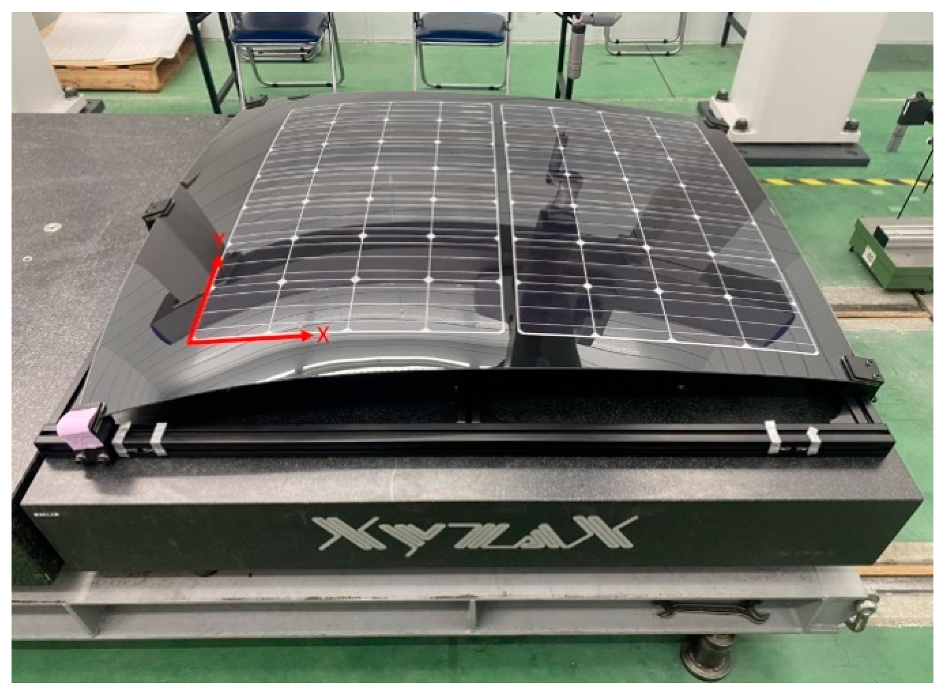
• The framed module is placed on a CMM surface plate (attached to the frame to prevent bending deformation).
• To verify the reference plane of the surface plate, a stylus is dropped on the surface plate near the four corners of the frame, and the height of the surface plate is measured (at four points; the Z value). Two points where the height of the surface plate is at the minimum and maximum are selected. The inclination of the line connecting the two points from the XY plane of the CMM coordinate system is calculated. No problems occur when the inclination is less than 0.1°.
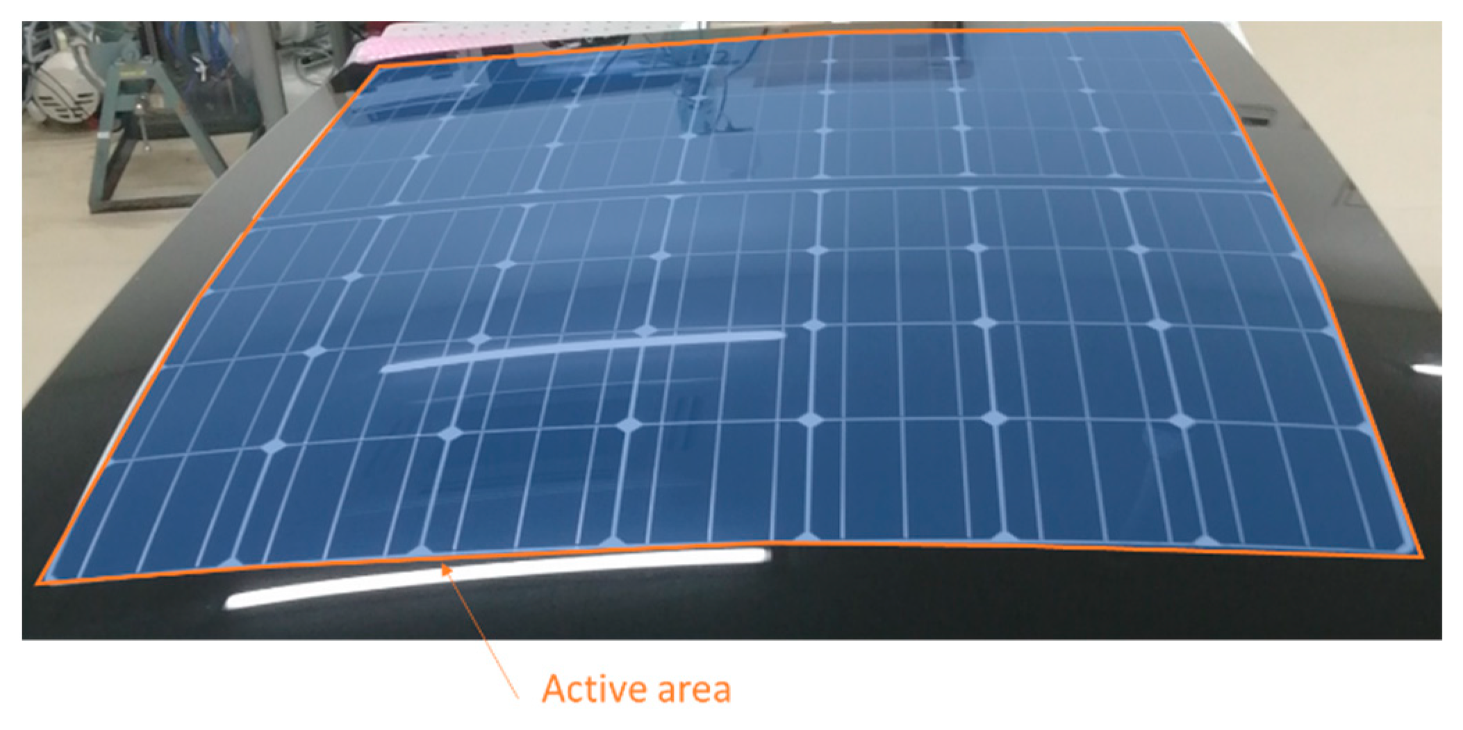
• The X- and Y-axes are defined with the vertex closest to the mechanical origin of the CMM as the origin within the envelope surface of the approximately rectangular area covered by the cell (Figure 4 and the active zone defined in Figure 5). In addition, the Z-axis in the vertical direction (upward) is considered, and the X-, Y-, and Z-axes are left-handed.
• The height is measured from the plate surface of the origin. Let this be dimension A.
• Let N and M be the number of rows and columns, respectively, of cells in an approximately rectangular area. The (2N + 1) and (2M + 1) measurement points are divided uniformly, including the edges of the rectangular region. All the (2N + 1) × (2M + 1) Z coordinates are measured. The arithmetic mean is the B-dimension (Figure 6 and ①–⑥).
• The offset of the reference plane for the indoor test (the length indicating how close the reference surface is to the light source from the bottom of the frame) is calculated as (A + B).

Figure 5. Definition of the active area and positional relationship to the mechanical contact points.

Figure 5. Definition of the active area and positional relationship to the mechanical contact points.

Figure 6. Coordinate measurement of the curved PV modules.

Figure 6. Coordinate measurement of the curved PV modules.

The position of the reference plane for the indoor measurement is given by the center of gravity of the active zone of the PV module parallel to the mechanical contact points of the module (Figure 5 and Figure 7), rather than by the mechanical contact points of the module or the peak position of the module.

The coordinate point of the average value of the X and Y coordinates in the cell coordinate measurement by the CMM was set as the center point of the module on the reference plane. The optical axis of the solar simulator was aligned accordingly.

The envelope surface of the approximately rectangular area covered by the cell should not protrude from the uniformly illuminated area of the reference surface.

In the case of a module in which the cells are arranged at equal intervals, the center point of the enveloping surface of the approximately rectangular area covered by the cells is regarded as the center point of the module. Even if it is not calculated from the CMM measurement values, the optical axis of the solar simulator may be aligned with this.

That the envelope surface of the approximately rectangular area covered by the cell should not protrude from the uniformly illuminated area of the reference surface.

This measurement is analogous to that of single-junction PV devices. For the solar simulators, the only adjustment is that of the total irradiance intensity (considering the associated variation in the spectral irradiance).

After the indoor test with the solar simulators, the actual output power was compared using the monitored power output (Figure 8).

First, an outdoor testbed was set at a given orientation angle, and the reference plane was adjusted horizontally. The carrier (holding fixture) was then placed on the reference plane while maintaining angles equal to those in the coordinate measurement and indoor performance test. The output power was monitored from sunrise to sunset while keeping the module orientations constant by scanning the load resistance and generating I-V and P-V curves. The output power was determined by identifying the peak in the P-V curve.

3. Results

This chapter discusses the unusual behavior of curved PV devices and explains it using the calculation model discussed in the previous chapter and its validation. The differences in indoor testing should be addressed by the differences discussed and described in several publications [65,67,68,69,94,95]. However, they mainly discussed whether the outdoor performance can be predicted using the indoor test results. After correcting for solar irradiance and device temperature, the outdoor power output of the flat PV devices was equal to the tested values. However, curved PV devices inherently differ.

3.1. General Behaviors of the Curved PV Devices

The outdoor monitoring of the commercial curved PV module (Figure 8) revealed a distinct difference caused by climatic conditions (Figure 9).

Diffuse solar irradiance was dominant on rainy or cloudy days. Thus, the variation among solar cells in the curved surface was marginal. Clear-sky days corresponded to solar irradiance originating from direct sunlight. Hence, the variation in cosine loss was considerable and caused a substantial mismatching loss.

The most distinct difference was observed in the fill factor (FF) behavior. The output power is the product of the short-circuit current Isc, open-circuit voltage Voc, and fill factor (FF): Pm = Isc × Voc × FF. In principle, the FF is almost constant in the range of Isc except for the small Isc region. This is owing to a relatively higher recombination ratio than the minority carrier injection. This was also observed in curved PV devices in cloudy and rainy climates. However, this trend varied significantly on clear-sky days. The FF was substantially reduced and decreased further at low Isc values, i.e., low height times. This, in turn, caused a significant power loss (Figure 9). On rainy or cloudy days, most of the solar irradiance originated from diffuse sunlight. Thus, the variation among the solar cells on the curved surface was marginal. Meanwhile, on clear-sky days, most solar irradiance originated from direct sunlight. Thus, the variation in cosine loss was substantial and resulted in a substantial mismatching loss. The FF loss in the low-Isc region on clear-sky days was considerable. This substantially reduced the power output.

The new computation approach powerfully explains the unusual behavior of the curved PV devices on clear-sky days. However, the same algorithm can be applied to rainy or cloudy days. In the next section of the experimental results, clear-sky and rainy or cloudy days were compared to the calculated results.

3.2. Validation of the Algorithms

As shown in Figure 9, curved PV devices occasionally generate a significant power loss owing to the inherent mismatch loss caused by the variations in the cosine loss from direct sunlight. Unlike flat PV devices, the power output in an actual outdoor operation inherently differs from the power output or efficiency values obtained from indoor testing with temperature and irradiance corrections. The question was whether the geometrical and circuit models could precisely estimate the difference in the vector computation model in Figure 2.

The vector computation model in Figure 2 was validated by outdoor monitoring of the power output from sunrise to sunset under various climatic conditions and orientations of the PV model (commercial VIPV product for the Toyota Prius 40 series). The results are shown in Figure 10 (clear-sky days) and Figure 11 (cloudy days).

The purple lines in Figure 10 represent the conventional power calculations assuming that the PV device is flat. These correct the module temperature and solar irradiance (global horizontal irradiance, GHI). These were overestimated on clear-sky days owing to the mismatching losses among the solar cells on the curved surface affected by the variations in the cosine losses. However, the result of the vector computation using the algorithm in Figure 2 matched the measured results (blue region) regardless of the orientation of the PV module.

This trend varied on cloudy days, when diffuse sunlight was dominant. The difference between the flat and curved models was insignificant, and both matched the measured trend. The exception was that the level of solar irradiance was high with a certain portion of direct sunlight (see the measurement on 15 March 2023 in Figure 11). In addition, the solar irradiance (GHI and DNI measurements) was measured on the building roof approximately 300 m north of the tested PV module. Thus, the solar irradiance may not be equal to the on-plane irradiance of the PV device (see morning and evening on 21 March 2023 and 17 March 2023 in Figure 11).

4. Discussion

We presented two types of vector computation algorithms for curved PV devices affected by non-uniform solar irradiance (Figure 1 and Figure 2). Figure 1 shows a rigorous model, and Figure 2 shows a simplified model that was applied to the following cases:

• The attitude and position are unaltered during the timeframe of the power measurement.
• The solar irradiance angular distribution is unaltered during the power measurement timeframe.
• The surface is a simple concave shape (not saddle-shaped or with multiple peaks, such as a twin bubble roof) [101,102].
• All the solar cells are connected in series.
• The nonlinear effects in equivalent circuits in the solar cells are negligible [103,104].
• The spectrum mismatching loss is negligible [105,106,107].
• The dynamic and partial shadings are negligible [108,109,110].

With respect to its application to VIPVs, it can be used for solar panels on a car roof (but not for advanced aero-designed roofs such as double bubbles). For solar panels on the engine or side of the car, the rigorous algorithm shown in Figure 1 should be used. In this study, the computational model was validated using the algorithm shown in Figure 2. Therefore, the indoor measurements of curved VIPV products for car roofs can be used to predict their outdoor performance.

Although this method was developed for the power estimation of curved PV devices, it can also be used to estimate the energy yield because the annual energy yield correlates with the energy yield’s actual value. To calculate the energy yield, the power of the photovoltaic device is typically calculated every hour based on a solar database such as the METPV series [111,112] considering the position of the sun relative to the device. Its power value is then integrated, multiplied, and weighted by the timeframe (typically 1 h).

The models shown in Figure 1 and Figure 2 can be used for other advanced integrations of photovoltaic devices:

• Wavy PV arrays that are installed in hilly areas where the performance ratio decreases in winter owing to self-shading by the PV arrays and irregular skylines can use the algorithm shown in Figure 1;
• Aircraft including drones and high-altitude platform systems (HAPS) can use the algorithm shown in Figure 1;
• BIPVs with multiplexed wall shading and self-shading by irregular or nonplanar PV arrays can use the algorithm shown in Figure 1;
• In flexible and film-type PV devices enclosing non-planar structures (Figure 1 and Figure 2);
• In photosynthetic photon flux density (PPFD) distribution calculations for crops grown below agriphotovoltaic systems.

This study, in particular, considered how PV devices behave and are affected by the surface profile (inherent properties). However, the performance of PV devices is affected by external factors like shading, including partial and dynamic shading. These factors are not typically used to describe product performance but are referenced in the energy yield discussion. Such evaluations were discussed in international standardization activities [113,114]. These algorithms and the testing and validation procedures, including safety issues with installing PV devices on the car body, are also discussed within the framework of international standardization [113,114].

The story of international standardization activity started in July 2017 with a web meeting of a group of researchers and testing engineers in PV industries to seek a solution for the measurement errors and different behaviors of curved PV devices from flat ones. The group gradually expanded, inviting experts from testing laboratories and engineers from the automotive industry seeking applications for automobile PV devices. In April 2021, it was upgraded to an official international project team (PT600) under the International Electrotechnical Commission (IEC) umbrella.

Most formulas, equations, modeling, and measurement methods for photovoltaic devices are based on the assumption that photovoltaic devices are flat, static (with no movement), and illuminated by uniform sunlight. It is a reasonable assumption for typical applications such as rooftop solar panels, but it cannot be applied to vehicle photovoltaic devices. For example, one of the essential equations (Power output) = (Power conversion efficiency) × (Area of the device) × (Solar irradiance) is not true for the car applications in a physically and mathematically rigorous manner. Such deviation affects the testing procedure. The deviation in PV device performance on vehicles is sometimes called “unusual behaviors”. Accurate modeling needs to be developed to understand these strange behaviors.

On the contrary, such advanced modeling requires advanced math, so not everyone can handle it, and often, it is not transparent when rating the product value. A simple approximation method is needed for rating purposes. Therefore, our standardization activity deals with three layers of testing and rating methodologies (

Table 2. The standardization activity on which this study was based consists of three layers of international activities.

Layer	Category	Goal
Layer 1	Product testing	Reproducibility among testing laboratories
Layer 2	Operating modeling	Accuracy (affected by shadows and curved surface)
Layer 3	Energy rating	Transparency (everyone can perform calculations)

). We need three layers because reproducible tests can only be secured in testing laboratories. Still, outdoor operation results are inherently different from test results (in principle, the test result is the same as the outdoor operation in flat PV devices after temperature and spectrum corrections). Note that most of the formula and testing methods are based on the assumption that the PV device is flat. Still, we need practical and reproducible testing methods (that are at least applicable by controlled testing laboratories, layer 1).

Unlike the flat PV devices (where the outdoor performance will be the same if sufficient corrections like temperature are performed), the behavior of the outdoor operation of curved PV modules is challenging to understand (most operation models are based on the assumption that PV devices are flat). We need a detailed translation procedure for outdoor operations to avoid misleading or unfair recognition. This is why we need layer 2.

A thorough and accurate calculation requires a tensor-matrix-vector computation, which not everyone can perform. Moreover, VIPVs frequently work in shaded and partially shaded environments. Therefore, we must provide an approximated but simple and transparent calculation procedure for a fair rating of the VIPV and SEV values (possibly related to carbon offset values). This is why we need layer 3.

The geometrical conditions and coordinate system (local coordinate system) can be applied to building-integrated photovoltaics (BIPVs), aircraft PVs, and PV arrays installed on wavy land. Except for reducing the requirements of the geometrical properties, the models and equations and Scheme 1 in Section 2.2, Section 2.3 and Section 2.4 cover the entire situation. The differences are summarized as follows.

BIPVs: The elevation angles are typically fixed to 90°, a particular case in the algorithm. PV devices usually do not move, which is also a specific case in the algorithm. The shading (aperture) matrix issue varies with the position of the PV arrays and can be covered by allocating the different matrixes depending on the device’s height (typically).

Aircraft PVs: The surface model defined in Section 2.4 can be applied to the saddle-curved surfaces that are typical in aircraft wings. As explained in Section 2.5, we also need to consider the hidden surface.

PV arrays installed on wavy land: The envelope of the PV arrays is regarded as the curved surface of the PV device, and the mismatching losses are considered to be constrained by the conservation law of the carriers in a series circuit. The aperture matrix can describe the shading effects of the sloped land [71].

This paper showed the validation result in vehicle applications using c-Si solar cells. However, the model was also tested by HAPS (High Altitude Platform Station), namely using drones. The PV devices made of GaAs and InGaP/GaAs/InGaAs triple junctions were used to cover the saddle-shaped curved wings for flying in the stratosphere using Figure 1, in namely different applications, curved shapes, solar cells, cell materials, and solar environments [102].

We did not explicitly consider bifacial panels. However, considering the front and back sides, this can be handled independently. In this case, if the front surface is convex, the rear surface will be concave, meaning that at least one side needs to be considered as the hidden surface.

Typical curved PV devices are 1.5 m and have a larger radius of curvature that is at least three orders larger than the thickness of the absorption layer (200 μm to 20 nm) and also have less than the typical deflection of the wafers that are not supported by a substrate or have a superstrength structure caused by internal stress (natural deflection). On the other hand, the tangent angle variation typically lies within more than ten orders of magnitude, which certainly affects the optical performance of the absorbers.

In this regard, the microscopic physics of PV devices, including differences in the materials, can be ignored or have substantially less impact than the differential geometry impact, including optical and circuit impacts. It is not necessary to think that curving might introduce a second wavelength photon that can be absorbed (for example, one-photon or two-photon absorption).

5. Conclusions

Most equations and models of photovoltaics (PVs) are based on the assumption that such devices are flat. The classical models based on flat PV devices do not consider the possibility of the local variations of cosine losses in the active area of PV devices and the mismatching losses in flat devices caused by this variation. Another misleading aspect is that the aperture area may be the same as the active area of flat PV devices, but this is not true for curved PV devices. The fundamental formula of PV devices, (Output) = (Device Active Area) × (Irradiance) × (Power Conversion Efficiency), is suitable for flat PV devices but incorrect for curved PV devices. Moreover, we do not have clear definitions of the area of the curved PV devices, including whether the projected or total active area should be used. This is an issue that the international web meeting groups, consisting of experts and researchers from research institutes, testing laboratories, and the PV and automotive industries, have discussed. The global meeting group was upgraded to an official international project team (PT600) under the umbrella of the International Electrotechnical Commission (IEC) in April 2021 and is continuing discussions for the goal of fair and scientifically correct international standards in this field.

The actual performance of nonplanar PV devices should be investigated and developed. In this study, outdoor monitoring was developed, and algorithms were validated based on vector computations. The measurement methods were also developed independently of this study by an international collaboration with testing laboratories for reproducible indoor test protocols. Note that reproducible tests were established for flat PV devices. Still, developing reproducible testing methods, including the additional testing equipment requirements, was challenging because most testing methods and instruments were designed for flat PV devices and did not work with sufficient reproducibility for curved PV devices.

In parallel with the above activities, we developed two models (Figure 1 and Figure 2). Both were based on differential geometry and were essentially the same. Still, the first one is more general and can be applied to the 3D movement of PV devices, such as an aircraft PV device (pitch, roll, and yaw rotations), but with more computation time. The second one is quick but can be applied to simple string configurations (all in series). It is limited to yaw movement and is suitable for vehicle applications. Also, note that the unusual behavior of the curved PV devices was enhanced on clear-sky days when the solar irradiance mainly consisted of direct and collimated sunlight, as anticipated. The developed models help us to understand the dramatic differences in the behaviors on clear-sky days from indoor-tested results.

References

1. Bogdanov, D.; Farfan, J.; Sadovskaia, K.; Aghahosseini, A.; Child, M.; Gulagi, A.; Oyewo, A.S.; de Souza Noel Simas Barbosa, L.; Breyer, C. Pathway towards sustainable electricity: Radical transformation via evolutionary transition steps. Nat. Commun. 2019, 10, 1077. [Google Scholar] [CrossRef] [PubMed]
2. Brown, T.W.; Bischof-Niemz, T.; Blok, K.; Breyer, C.; Lund, H.; Mathiesen, B.V. Response to ‘burden of proof: A comprehensive review of the feasibility of 100% renewable-electricity systems’. Renew. Sustain. Energy Rev. 2018, 92, 834–847. [Google Scholar] [CrossRef]
3. Ram, M.; Bogdanov, D.; Aghahosseini, A.; Solomon, O.A.; Gulagi, A.; Child, M.; Fell, H.-J.; Breyer, C. Global Energy System Based on 100% Renewable Energy-Power Sector. Study by Lappeenranta University of Technology and Energy Watch Group, Lappeenranta and Berlin. 2017. Available online: https://goo.gl/7y9sKR (accessed on 15 May 2024).
4. Breyer, C.; Bogdanov, D.; Aghahosseini, A.; Gulagi, A.; Child, M.; Oyewo, A.S.; Farfan, J.; Sadovskaia, K.; Vainikka, P. Solar photovoltaics demand for the global energy transition in the power sector. Prog. Photovolt. Res. Appl. 2017, 26, 505–523. [Google Scholar] [CrossRef]
5. Khalili, S.; Rantanen, E.; Bogdanov, D.; Breyer, C. Global Transportation Demand Development with Impacts on the Energy Demand and Greenhouse Gas Emissions in a Climate-Constrained World. Energies 2019, 12, 3870. [Google Scholar] [CrossRef]
6. García-Olivares, A.; Solé, J.; Osychenko, O. Transportation in a 100% renewable energy system. Energ. Convers. Manag. 2018, 158, 266–285. [Google Scholar] [CrossRef]
7. Breyer, C.; Khalili, S.; Bogdanov, D. Solar photovoltaic capacity demand for a sustainable transport sector to fulfil the Paris Agreement by 2050. Prog. Photovolt. Res. Appl. 2019, 27, 978–989. [Google Scholar] [CrossRef]
8. Wang, D.; Sechilariu, M.; Locment, F. PV-Powered Charging Station for Electric Vehicles: Power Management with Integrated V2G. Appl. Sci. 2020, 10, 6500. [Google Scholar] [CrossRef]
9. Sayed, K.; Abo-Khalil, A.G.; Alghamdi, A.S. Optimum Resilient Operation and Control DC Microgrid Based Electric Vehicles Charging Station Powered by Renewable Energy Sources. Energies 2019, 12, 4240. [Google Scholar] [CrossRef]
10. Wang, D.; Locment, F.; Sechilariu, M. Modelling, Simulation, and Management Strategy of an Electric Vehicle Charging Station Based on a DC Microgrid. Appl. Sci. 2020, 10, 2053. [Google Scholar] [CrossRef]
11. Yao, L.; Damiran, Z.; Lim, W.H. Optimal Charging and Discharging Scheduling for Electric Vehicles in a Parking Station with Photovoltaic System and Energy Storage System. Energies 2017, 10, 550. [Google Scholar] [CrossRef]
12. Dai, Q.; Liu, J.; Wei, Q. Optimal Photovoltaic/Battery Energy Storage/Electric Vehicle Charging Station Design Based on Multi-Agent Particle Swarm Optimization Algorithm. Sustainability 2019, 11, 1973. [Google Scholar] [CrossRef]
13. Araki, K.; Nagai, H.; Yamaguchi, M. September. Possibility of solar station to EV. In AIP Conference Proceedings; AIP Publishing LLC: Melville, NY, USA, 2016; Volume 1766, p. 080001. [Google Scholar]
14. Araki, K.; Ji, L.; Kelly, G.; Yamaguchi, M. To do list for research and development and international standardization to achieve the goal of running a majority of electric vehicles on solar energy. Coatings 2018, 8, 251. [Google Scholar] [CrossRef]
15. [IEA PVPS]—International Energy Agency Photovoltaic Power System Programme. PV for Transport, IEA PVPS Task 17. St. Ursen: IEA PVPS. 2018. Available online: http://www.iea-pvps.org/index.php?id=484 (accessed on 15 May 2024).
16. Sono Motors. Sion—Infinite Mobility, Munich. 2018. Available online: https://sonomotors.com/sion.html/ (accessed on 15 May 2024).
17. Jeon, S.; Choung, S.; Bae, S.; Choi, J.; Shin, D. Analysis on Power Generation Characteristics of a Vehicle Rooftop Photovoltaic Module with Urban Driving Conditions. Tran. Korean Inst. Power Electron. 2020, 25, 79–86. [Google Scholar]
18. Schuss, C.; Fabritius, T.; Eichberger, B.; Rahkonen, T. Energy-efficient Routing of Electric Vehicles with Integrated Photovoltaic Installations. In Proceedings of the 2020 IEEE International Instrumentation and Measurement Technology Conference (I2MTC), Dubrovnik, Croatia, 25–28 May 2020; pp. 1–6. [Google Scholar] [CrossRef]
19. Letendre, S.; Perez, R.; Herig, C. Vehicle integrated PV: A clean and secure fuel for hybrid electric vehicles. In Proceedings of the Solar Conference; American Solar Energy Society: Boulder, CO, USA; American Institute of Architects: Washington, DC, USA, 2003; pp. 201–206. [Google Scholar]
20. Kim, J.; Wang, Y.; Pedram, M.; Chang, N. Fast photovoltaic array reconfiguration for partial solar powered vehicles. In Proceedings of the International Symposium on Low Power Electronics and Design, La Jolla, CA, USA, 11–13 August 2014; pp. 357–362. [Google Scholar]
21. Araki, K.; Sato, D.; Masuda, T.; Lee, K.H.; Yamada, N.; Yamaguchi, M. Why and how does car-roof PV create 50 GW/year of new installations? Also, why is a static CPV suitable to this application? In AIP Conference Proceedings; AIP Publishing LLC: Melville, NY, USA, 2019; Volume 2149, Number 1; p. 050003. [Google Scholar]
22. De Pinto, S.; Lu, Q.; Camocardi, P.; Chatzikomis, C.; Sorniotti, A.; Ragonese, D.; Iuzzolino, G.; Perlo, P.; Lekakou, C. Electric vehicle driving range extension using photovoltaic panels. In Proceedings of the IEEE Vehicle Power and Propulsion Conference (VPPC), Hangzhou, China, 17–20 October 2016; IEEE: Piscataway, NJ, USA, 2016; pp. 1–6. [Google Scholar]
23. Fujinaka, M. The practically usable electric vehicle charged by photovoltaic cells. In Proceedings of the 24th Intersociety Energy Conversion Engineering Conference, Washington, DC, USA, 6–11 August 1989; IEEE: Piscataway, NJ, USA, 2002; pp. 2473–2478. [Google Scholar]
24. Ezzat, M.F.; Dincer, I. Development, analysis and assessment of a fuel cell and solar photovoltaic system powered vehicle. Energy Convers. Manag. 2016, 129, 284–292. [Google Scholar] [CrossRef]
25. Talluri, G.; Grasso, F.; Chiaramonti, D. Is Deployment of Charging Station the Barrier to Electric Vehicle Fleet Development in EU Urban Areas? An Analytical Assessment Model for Large-Scale Municipality-Level EV Charging Infrastructures. Appl. Sci. 2019, 9, 4704. [Google Scholar] [CrossRef]
26. Alhammad, Y.A.; Al-Azzawi, W.F. Exploitation the waste energy in hybrid cars to improve the efficiency of solar cell panel as an auxiliary power supply. In Proceedings of the 10th International Symposium on Mechatronics and its Applications (ISMA), Sharjah, United Arab Emirates, 8–10 December 2015; IEEE: Piscataway, NJ, USA, 2016; pp. 1–6. [Google Scholar]
27. Naves, A.X.; Tulus, V.; Vazquez, E.G.; Esteller, L.J.; Haddad, A.N.; Boer, D. Economic Optimization of the Energy Supply for a Logistics Center Considering Variable-Rate Energy Tariffs and Integration of Photovoltaics. Appl. Sci. 2019, 9, 4711. [Google Scholar] [CrossRef]
28. Pavlovic, A.; Sintoni, D.; Fragassa, C.; Minak, G. Multi-Objective Design Optimization of the Reinforced Composite Roof in a Solar Vehicle. Appl. Sci. 2020, 10, 2665. [Google Scholar] [CrossRef]
29. Samadi, H.; Ala, G.; Lo Brano, V.; Romano, P.; Viola, F. Investigation of Effective Factors on Vehicles Integrated Photovoltaic (VIPV) Performance: A Review. World Electr. Veh. J. 2023, 14, 154. [Google Scholar] [CrossRef]
30. Araki, K.; Ota, Y.; Saiki, H.; Tawa, H.; Nishioka, K.; Yamaguchi, M. Super-Multi-Junction Solar Cells—Device Configuration with the Potential for More Than 50% Annual Energy Conversion Efficiency (Non-Concentration). Appl. Sci. 2019, 9, 4598. [Google Scholar] [CrossRef]
31. Yamaguchi, M.; Ozaki, R.; Nakamura, K.; Lee, H.; Kojima, N.; Ohshita, Y.; Masuda, T.; Okumura, K.; Satou, A.; Nakado, T.; et al. Development of High-Efficiency Solar Cell Modules for Photovoltaic-Powered Vehicles. Sol. RRL 2022, 6, 2100429. [Google Scholar] [CrossRef]
32. Vadgama, T.N.; Patel, M.A.; Thakkar, D.D. Design of Formula One Racing Car. Int. J. Eng. Res. Technol. 2015, 4, 702–712. [Google Scholar]
33. Ustun, O.; Yilmaz, M.; Gokce, C.; Karakaya, U.; Tuncay, R.N. Energy management method for solar race car design and application. In Proceedings of the 2009 IEEE International Electric Machines and Drives Conference, Madison, WI, USA, 3–6 May 2009; pp. 804–811. [Google Scholar]
34. Minak, G.; Fragassa, C.; de Camargo, F.V. A Brief Review on Determinant Aspects in Energy Efficient Solar Car Design and Manufacturing. In Sustainable Design and Manufacturing (SDM) 2017; Campana, G., Ed.; Smart Innovation, Systems and Technologies; Springer: Cham, Switzerland, 2017; Volume 68, pp. 847–856. [Google Scholar]
35. Odabasi, V.; Maglio, S.; Martini, A.; Sorrentino, S. Static stress analysis of suspension systems for a solar-powered car. FME Trans. 2019, 47, 70–75. [Google Scholar] [CrossRef]
36. Betancur, E.; Fragassa, C.; Coy, J.; Hincapie, S.; Osorio, G. Aerodynamic effects of manufacturing tolerances on a solar car. In Proceedings of the International Conference on Sustainable Design and Manufacturing, Bologna, Italy, 26–28 April 2002; pp. 868–876. [Google Scholar]
37. Beardmore, P.; Johnson, C.F. The potential for composites in structural automotive applications. Compos. Sci. Technol. 1986, 26, 251–281. [Google Scholar] [CrossRef]
38. Nagavally, R.R. Composite materials-history, types, fabrication techniques, advantages, and applications. Int. J. Mech. Prod. Eng. 2017, 5, 82–87. [Google Scholar]
39. Yang, R.J.; Chahande, A.I. Automotive applications of topology optimization. Struct. Optim. 1995, 9, 245–249. [Google Scholar] [CrossRef]
40. Cavazzuti, M.; Splendi, L.; D’Agostino, L.; Torricelli, E.; Costi, D.; Baldini, A. Structural optimization of automotive chassis: Theory, set up, design. In Problemes Inverses, Controle et Optimisation de Formes; Université Paris-Dauphine: Paris, France, 2012; Volume 6. [Google Scholar]
41. Cavazzuti, M.; Baldini, A.; Bertocchi, E.; Costi, D.; Torricelli, E.; Moruzzi, P. High performance automotive chassis design: A topology optimization based approach. Struct. Multidiscip. Optim. 2011, 44, 45–56. [Google Scholar] [CrossRef]
42. Zhu, P.; Zhang, Y.; Chen, G.L. Metamodel-based lightweight design of an automotive front-body structure using robust optimization. Proc. Inst. Mech. Eng. Part D J. Automob. Eng. 2009, 223, 1133–1147. [Google Scholar] [CrossRef]
43. Yildiz, A.R. A new hybrid particle swarm optimization approach for structural design optimization in the automotive industry. Proc. Inst. Mech. Eng. Part D J. Automob. Eng. 2012, 226, 1340–1351. [Google Scholar] [CrossRef]
44. Ermolaeva, N.S.; Castro, M.B.; Kandachar, P.V. Materials selection for an automotive structure by integrating structural optimization with environmental impact assessment. Mater. Des. 2004, 25, 689–698. [Google Scholar] [CrossRef]
45. Minak, G.; Brugo, T.M.; Fragassa, C.; Pavlovic, A.; Zavatta, N.; De Camargo, F. Structural Design and Manufacturing of a Cruiser Class Solar Vehicle. J. Vis. Exp. 2019, 143, e58525. [Google Scholar]
46. Cross, N.; Cross, A.C. Winning by design: The methods of Gordon Murray, racing car designer. Des. Stud. 1996, 17, 91–107. [Google Scholar] [CrossRef]
47. Holmberg, K.; Andersson, P.; Erdemir, A. Global energy consumption due to friction in passenger cars. Tribol. Int. 2012, 47, 221–234. [Google Scholar] [CrossRef]
48. Joost, W. Reducing vehicle weight and improving U.S. energy efficiency using integrated computational materials engineering. J. Miner Met. Mater. Soc. 2012, 64, 1032–1038. [Google Scholar] [CrossRef]
49. Elmarakbi, A. Advanced Composite Materials for Automotive Applications: Structural Integrity and Crashworthiness; John Wiley & Sons: Hoboken, NJ, USA, 2013. [Google Scholar]
50. Parkinson, A.R.; Balling, R.; Hedengren, J.D. Optimization Methods for Engineering Design; Brigham Young University: Provo, UT, USA, 2013. [Google Scholar]
51. Kim, C.H.; Mijar, A.R.; Arora, J.S. Development of simplified models for design and optimization of automotive structures for crashworthiness. Struct. Multidiscip. Optim. 2001, 22, 307–321. [Google Scholar] [CrossRef]
52. Muyl, F.; Dumas, L.; Herbert, V. Hybrid method for aerodynamic shape optimization in automotive industry. Comput. Fluids 2004, 33, 849–858. [Google Scholar] [CrossRef]
53. Nikbakt, S.; Kamarian, S.; Shakeri, M. A review on optimization of composite structures Part I: Laminated composites. Compos. Struct. 2018, 195, 158–185. [Google Scholar] [CrossRef]
54. Dos Santos, F.L.M.; Peeters, B.; Menchicchi, M.; Lau, J.; Gielen, L.; Desmet, W.; Góes, L.C.S. Strain-based dynamic measurements and modal testing. In Topics in Modal Analysis II; Allemang, R., Ed.; Springer: Cham, Switzerland, 2014; Volume 8, pp. 233–242. [Google Scholar]
55. Wloch, K.; Bentley, P.J. Optimising the performance of a formula one car using a genetic algorithm. In International Conference on Parallel Problem Solving from Nature; Springer: Berlin/Heidelberg, Germany, 2004; pp. 702–711. [Google Scholar]
56. De Kock, J.P.; van Rensburg, N.J.; Kruger, S.; Laubscher, R.F. Aerodynamic optimization in a lightweight solar vehicle design. In Proceedings of the ASME International Mechanical Engineering Congress and Exposition, Montreal, QC, Canada, 14–20 November 2017; pp. 1–8. [Google Scholar]
57. Kudo, Y.; Sato, A.; Kimura, K.; Iwamoto, S.; Ohba, H.; Sakabe, M.; Shirai, Y. Solar module laminated constitution for automobiles. In Proceedings of the SAE 2016 World Congress and Exhibition, Detroit, MI, USA, 12–14 April 2016. [Google Scholar]
58. Alpuerto, L.; Balog, R.S. Comparing Connection Topologies of PV Integrated Curved Roof Tile for Improved Performance. In Proceedings of the 2020 IEEE Texas Power and Energy Conference (TPEC), College Station, TX, USA, 6–7 February 2020; pp. 1–5. [Google Scholar]
59. Walker, G.R.; Xue, J.; Sernia, P. PV string per-module maximum power point enabling converters. In Proceedings of the Australasian Universities Power Engineering Conference (AUPEC’03), Christchurch, New Zealand, 28 September—1 October 2003. [Google Scholar]
60. Benlekkam, M.; Nehari, D.; Madani, H.I. Enhancement of the thermal regulation performance of a curved PV panel. Int. J. Renew. Energy Res. 2017, 7, 707–714. [Google Scholar]
61. Sato, D.; Masuda, T.; Araki, K.; Yamaguchi, M.; Okumura, K.; Sato, A.; Tomizawa, R.; Yamada, N. Stretchable micro-scale concentrator photovoltaic module with 15.4% efficiency for three-dimensional curved surfaces. Commun. Mater. 2021, 2, 7. [Google Scholar] [CrossRef]
62. Commault, B.; Duigou, T.; Maneval, V.; Gaume, J.; Chabuel, F.; Voroshazi, E. Overview and Perspectives for Vehicle-Integrated Photovoltaics. Appl. Sci. 2020, 11, 11598. [Google Scholar] [CrossRef]
63. Wheeler, A.J.; Leveille, M.; Kurtz, S.; Anton, I.; Limpinsel, M. Outdoor Performance of PV Technologies in Simulated Automotive Environments. In Proceedings of the 2019 IEEE 46th Photovoltaic Specialists Conference (PVSC), Chicago, IL, USA, 16–21 June 2019. [Google Scholar]
64. Wheeler, A.; Leveille, M.; Anton, I.; Leilaeioun, A.; Kurtz, S. Determining the Operating Temperature of Solar Panels on Vehicles. In Proceedings of the 2019 IEEE 46th Photovoltaic Specialists Conference (PVSC), Chicago, IL, USA, 16–21 June 2019. [Google Scholar]
65. Ota, Y.; Masuda, T.; Araki, K.; Yamaguchi, M. Curve-correction factor for characterization of the output of a three-dimensional curved photovoltaic module on a car roof. Coatings 2018, 8, 432. [Google Scholar] [CrossRef]
66. Araki, K.; Ota, Y.; Nishioka, K.; Tobita, H.; Ji, L.; Kelly, G.; Yamaguchi, M. Toward the Standardization of the Car-roof PV–The challenge to the 3-D Sunshine Modeling and Rating of the 3-D Continuously Curved PV Panel. In Proceedings of the 2018 IEEE 7th World Conference on Photovoltaic Energy Conversion (WCPEC) (A Joint Conference of 45th IEEE PVSC, 28th PVSEC & 34th EU PVSEC), Waikoloa, HI, USA, 10–15 June 2018; pp. 0368–0373. [Google Scholar]
67. Araki, K.; Ota, Y.; Lee, K.H.; Yamada, N.; Yamaguchi, M. Curve Correction of the Energy Yield by Flexible Photovoltaics for VIPV and BIPV Applications Using a Simple Correction Factor. In Proceedings of the 2019 IEEE 46th Photovoltaic Specialists Conference (PVSC), Chicago, IL, USA, 16–21 June 2019; pp. 1584–1591. [Google Scholar]
68. Ota, Y.; Araki, K.; Nagaoka, A.; Nishioka, K. Facilitating vehicle-integrated photovoltaics by considering the radius of curvature of the roof surface for solar cell coverage. Clean. Eng. Technol. 2022, 7, 100446. [Google Scholar] [CrossRef]
69. Araki, K.; Ota, Y.; Nishioka, K. Testing and rating of vehicle-integrated photovoltaics: Scientific background. Sol. Energy Mater. Sol. Cells, 2024; in review. [Google Scholar]
70. Araki, K.; Ota, Y.; Maeda, A.; Kumano, M.; Nishioka, K. Solar Electric Vehicles as Energy Sources in Disaster Zones: Physical and Social Factors. Energies 2022, 16, 3580. [Google Scholar] [CrossRef]
71. Araki, K.; Ota, Y.; Nagaoka, A.; Nishioka, K. 3D Solar Irradiance Model for Nonuniform Shading Environments Using Shading (Aperture) Matrix Enhanced by Local Coordinate System. Energies 2022, 16, 4414. [Google Scholar] [CrossRef]
72. Kurtz, S.R.; O’Neill, M.J. Estimating and controlling chromatic aberration losses for two-junction, two-terminal devices in refractive concentrator systems. In Proceedings of the Conference Record of the Twenty Fifth IEEE Photovoltaic Specialists Conference, Washington, DC, USA, 13–17 May 1996; pp. 361–364. [Google Scholar]
73. James, L.W. Effects of concentrator chromatic aberration on multi-junction cells. In Proceedings of the 1994 IEEE 1st World Conference on Photovoltaic Energy Conversion-WCPEC (A Joint Conference of PVSC, PVSEC and PSEC), Waikoloa, HI, USA, 5–9 December 1994; pp. 1799–1802. [Google Scholar]
74. Sato, D.; Lee, K.H.; Araki, K.; Masuda, T.; Yamaguchi, M.; Yamada, N. Design of low-concentration static III-V/Si partial CPV module with 27.3% annual efficiency for car-roof application. Prog. Photovolt. Res. Appl. 2019, 27, 501–510. [Google Scholar] [CrossRef]
75. Rebeca, H.; Antón, I.; Victoria, M.; Domínguez, C.; Askins, S.; Sala, G.; De Nardis, D.; Araki, K. Experimental analysis and simulation of a production line for CPV modules: Impact of defects, misalignments, and binning of receivers. Energy Sci. Eng. 2017, 5, 257–269. [Google Scholar]
76. Herrero, R.; Antón, I.; Sala, G.; De Nardis, D.; Araki, K.; Yamaguchi, M. September. Monte Carlo simulation to analyze the performance of CPV modules. In AIP Conference Proceedings; AIP Publishing LLC: Melville, NY, USA, 2017; Volume 1881, p. 090001. [Google Scholar]
77. Araki, K.; Nagai, H.; Herrero, R.; Antón, I.; Sala, G.; Yamaguchi, M. Off-Axis Characteristics of CPV Modules Result From Lens-Cell Misalignment—Measurement and Monte Carlo Simulation. IEEE J. Photovolt. 2016, 6, 1353–1359. [Google Scholar] [CrossRef]
78. Araki, K.; Nagai, H.; Herrero, R.; Antón, I.; Sala, G.; Lee, K.H.; Yamaguchi, M. 1-D and 2-D Monte Carlo simulations for analysis of CPV module characteristics including the acceptance angle impacted by assembly errors. Sol. Energy 2017, 147, 448–454. [Google Scholar] [CrossRef]
79. Mangu, R.; Prayaga, K.; Nadimpally, B.; Nicaise, S. Design, Development and Optimization of Highly Efficient Solar Cars: Gato del Sol I–IV. In Proceedings of the 2010 IEEE Green Technologies Conference, Grapevine, TX, USA, 15–16 April 2010; pp. 1–6. [Google Scholar]
80. Araki, K.; Carr, A.J.; Chabuel, F.; Commault, B.; Derks, R.; Ding, K.; Duigou, T.; Ekins-Daukes, N.J.; Gaume, J.; Hirota, T.; et al. State-of-the-Art and Expected Benefits of PV-Powered Vehicles, International Energy Agency. 2021. Available online: https://iea-pvps.org/key-topics/state-of-the-art-and-expected-benefits-of-pv-powered-vehicles/ (accessed on 15 May 2024).
81. Heinrich, M.; Kutter, C.; Basler, F.; Mittag, M.; Alanis, L.E.; Eberlein, D.; Schmid, A.; Reise, C.; Kroyer, T.; Neuhaus, D.H.; et al. Potential and Challenges of Vehicle Integrated Photovoltaics for Passenger Cars. In Proceedings of the 37th European PV Solar Energy Conference and Exhibition, Lisbon, Portugal, 7–11 September 2020. [Google Scholar]
82. How to Install Flexible Solar Panels for Car Roof, Sungold. Available online: https://www.sungoldsolar.com/how-to-install-flexible-solar-panels-for-car-roof/ (accessed on 22 December 2023).
83. Bellini, E. Vehicle-Integrated Solar Kit May Reduce Frequency of Recharging by 14%. pv Magazine. Available online: https://www.pv-magazine-australia.com/2022/09/26/vehicle-integrated-solar-kit-may-reduce-frequency-of-recharging-by-14/ (accessed on 22 December 2023).
84. Solar Cells in Vehicles (VIPV): Between Research and Realism. IMEC. Available online: https://www.imec-int.com/en/articles/solar-cells-vehicles-vipv-between-research-and-realism (accessed on 22 December 2023).
85. Rosca, V.; Guillevin, N.; Okel, L.A.G.; Newman, B.K. Prefab Approach to Mass Customization. In Proceedings of the SiliconPV Conferenz, Konstanz, Germany, 28–30 March 2022. [Google Scholar]
86. Okel, L.A.G.; Guillevin, N.; Hoek, E.; Apaydin, O.; Rosca, V.; Newman, B.K. Manufacturing high-yield, low-cost, lightweight VIPV components. In Proceedings of the PVinMotion, ‘s-Hertogenbosch, The Netherlands, 15–17 February 2023. [Google Scholar]
87. Newman, B.K. Advances in conductive back sheet module technology for emerging applications. In Proceedings of the Back Contact Workshop, Munich, Germany, 12 May 2022. [Google Scholar]
88. Shukla, A.K.; Sudhakar, K.; Baredar, P. A comprehensive review on design of building integrated photovoltaic system. Energy Build. 2016, 128, 99–110. [Google Scholar] [CrossRef]
89. Jelle, B.P.; Breivik, C. State-of-the-art Building Integrated Photovoltaics. Energy Procedia 2012, 20, 68–77. [Google Scholar] [CrossRef]
90. Jelle, B.P.; Breivik, C. The path to the building integrated photovoltaics of tomorrow. Energy Procedia 2012, 20, 78–87. [Google Scholar] [CrossRef]
91. Commault, B.; Chambion, B.; Serra, L.; Karoui, F.; Nassibi, S. On-Board Photovoltaic Kit for Existing Vehicles. In Proceedings of the 8th World Conference on Photovoltaic Energy Conversion, Milano, Italy, 26–30 September 2022. [Google Scholar]
92. Duigou, T.; Caplet, S.; Chambion, B.; Gaume, J. Numerical simulation and experimental characterization of c-Si cells mechanical limits in spherical curvature shape. In Proceedings of the 38th EU PVSEC, Lisbon, Portugal, 6–10 September 2021. [Google Scholar]
93. Zhao, J.-H.; Tellkamp, J.; Gupta, V.; Edwards, D.R. Experimental Evaluations of the Strength of Silicon Die by 3-Point-Bend versus Ball-on-Ring Tests. IEEE Trans. Electron. Packag. Manuf. 2009, 32, 248–255. [Google Scholar] [CrossRef]
94. Araki, K.; Ota, Y.; Yamaguchi, M. Measurement and Modeling of 3D Solar Irradiance for Vehicle-Integrated Photovoltaic. Appl. Sci. 2020, 10, 872. [Google Scholar] [CrossRef]
95. Tayagaki, T.; Araki, K.; Yamaguchi, M.; Sugaya, T. Impact of nonplanar panels on photovoltaic power generation in the case of vehicles. IEEE J. Photovolt. 2019, 9, 1721–1726. [Google Scholar] [CrossRef]
96. Ota, Y.; Masuda, T.; Araki, K.; Yamaguchi, M. A mobile multipyranometer array for the assessment of solar irradiance incident on a photovoltaic-powered vehicle. Sol. Energy 2019, 184, 84–90. [Google Scholar] [CrossRef]
97. Araki, K.; Lee, K.H.; Masuda, T.; Hayakawa, Y.; Yamada, N.; Ota, Y.; Yamaguchi, M. Rough and Straightforward Estimation of the Mismatching Loss by Partial Shading of the PV Modules Installed on an Urban Area or Car-Roof. In Proceedings of the 2019 IEEE 46th Photovoltaic Specialists Conference (PVSC), Chicago, IL, USA, 16–21 June 2019; pp. 1218–1225. [Google Scholar]
98. Zhang, X.; Jin, C.; Hu, P.; Zhu, X.; Hou, W.; Xu, J.; Wang, C.; Zhang, Y.; Ma, Z.-D.; Smith, H. NURBS modeling and isogeometric shell analysis for complex tubular engineering structures. Comput. Appl. Math. 2017, 36, 1659–1679. [Google Scholar] [CrossRef]
99. Sußner, G.; Meyer, Q.; Greiner, G. High Quality Realtime Tessellation of Trimmed NURBS Surfaces for Interactive Examination of Surface Quality on Car Bodies. In Proceedings of the 17th International Meshing Roundtable; Garimella, R.V., Ed.; Springer: Berlin/Heidelberg, Germany, 2008. [Google Scholar] [CrossRef]
100. Sansoni, G.; Docchio, F. Three-dimensional optical measurements and reverse engineering for automotive applications. Robot. Comput. Integr. Manuf. 2004, 20, 359–367. [Google Scholar] [CrossRef]
101. Matsushita, S.; Araki, K.; Ota, Y.; Nishioka, K. Is a dpuble-bulbe curved-surface with excellent aerodynamics suitable for vhielce-integrated photovoltaic (VIPV) installations? In Proceedings of the EU PVSEC 2023, Lisbon, Portugal, 18–22 September 2023. [Google Scholar] [CrossRef]
102. Nishioka, K.; Okada, K.; Araki, K.; Kiyama, S.; Ota, Y.; Nishiyama, K. PV on HAPS (high altitude platform station): PV modeling. In Proceedings of the PVinMotion conference, Neuchatel, Switzerland, 6–8 March 2024. [Google Scholar]
103. Araki, K.; Yamaguchi, M.; Takamoto, T.; Ikeda, E.; Agui, T.; Kurita, H.; Takahashi, K.; Unno, T. Characteristics of GaAs-based concentrator cells. Sol. Energy Mater. Sol. Cells 2001, 66, 559–565. [Google Scholar] [CrossRef]
104. Araki, K.; Yamaguchi, M. Novel equivalent circuit model and statistical analysis in parameters identification. Sol. Energy Mater. Sol. Cells 2003, 75, 457–4661. [Google Scholar] [CrossRef]
105. Araki, K.; Yamaguchi, M.; Kondo, M.; Uozumi, H. Which is the best number of junctions for solar cells under ever-changing terrestrial spectrum? In Proceedings of the 3rd World Conference on Photovoltaic Energy Conversion, Osaka, Japan, 11–18 May 2003; Code 63772. pp. 307–312. [Google Scholar]
106. Tawa, H.; Saiki, H.; Ota, Y.; Araki, K.; Takamoto, T.; Nishioka, K. Accurate output forecasting method for various photovoltaic modules considering incident angle and spectral change owing to atmospheric parameters and cloud conditions. Appl. Sci. 2020, 10, 703. [Google Scholar] [CrossRef]
107. Araki, K.; Tawa, H.; Saiki, H.; Ota, Y.; Nishioka, K.; Yamaguchi, M. The outdoor field test and energy yield model of the four-terminal on Si tandem PV module. Appl. Sci. 2020, 10, 2529. [Google Scholar] [CrossRef]
108. Newman, B.K.; Burgers, A.R.; Dekker, N.J.J.; Manshanden, P.; Jansen, M.J.; Kester, J.C.P. Impact of Dynamic Shading in cSi PV Modules and Systems for Novel Applications. In Proceedings of the 2019 IEEE 46th Photovoltaic Specialists Conference (PVSC), Chicago, IL, USA, 16–21 June 2019. [Google Scholar]
109. Schuss, C.; Kotikumpu, T.; Eichberger, B.; Rahkonen, T. Impact of dynamic environmental conditions on the output behaviour of photovoltaics. In Proceedings of the 20th IMEKO TC-4 International Symposium, Benevento, Italy, 15–17 September 2014; pp. 993–998. [Google Scholar]
110. Schuss, C.; Gall, H.; Eberhart, K.; Illko, H.; Eichberger, B. Alignment and interconnection of photovoltaics on electric and hybrid electric vehicles. In Proceedings of the IEEE International Instrumentation and Measurement Technology Conference (I2MTC) Proceedings, Montevideo, Uruguay, 12–15 May 2014; pp. 153–158. [Google Scholar]
111. Itagaki, A.; Okumura, H.; Yamada, A. Preparation of meteorological data set throughout Japan for suitable design of PV systems Photovoltaic Energy Conversion. In Proceedings of the 3rd World Conference on Photovoltaic Energy Conversion, Osaka, Japan, 11–18 May 2003; Volume 2. [Google Scholar]
112. Shirakawa, K.; Itagaki, A.; Utsunomiya, T. Preparation of hourly solar radiation data on inclined surface (METPV-11) throughout Japan. In Proceedings of the JSES/JWEA Joint Conference, Wakkanai, Japan, 21–22 September 2011; pp. 193–196. [Google Scholar]
113. Araki, K.; Ji, L.; Kelly, G.; Ham, A.V.D.; Agudo, E.; Antón, I.; Baudrit, M.; Carr, A.; Herrero, R.; Kurtz, S.; et al. How did the knowledge of CPV contribute to the standardization activity of VIPV? In AIP Conference Proceedings; AIP Publishing LLC: Melville, NY, USA, 2020; Volume 2298, p. 060001. [Google Scholar]
114. Pravettoni, M.; Toto Brocchi, A. Towards a definition of standard test conditions for vehicle integrated photovoltaics. In Proceedings of the SNEC 2019 Scientific Conference, Shanghai, China, 5 June 2019. [Google Scholar]
Scheme 1. Structure of the aperture matrix.
Applsci 14 04855 sch001
Figure 1. The algorithm flowchart for computing the power output of a curved PV module affected by non-uniform solar irradiance and subjected to frequent movements in the local coordinate system [68].
Applsci 14 04855 g001
Figure 2. The simplified algorithm flowchart for computing the power output of a curved PV module [69].
Applsci 14 04855 g002
Figure 3. Carrier for the curved PV module. It was designed to keep angles equal during the following measurement steps: (1) coordinate measurements, (2) indoor performance tests, and (3) outdoor performance tests.
Applsci 14 04855 g003
Figure 4. Coordinate measurement of the curved PV modules with the carrier.
Applsci 14 04855 g004
Figure 7. Indoor tests with the carrier.
Applsci 14 04855 g007
Figure 8. Outdoor tests with the carrier.
Applsci 14 04855 g008
Figure 9. The trend of FF under different climatic conditions.
Applsci 14 04855 g009
Figure 10. Comparison of the outdoor power output determined using the indoor test result on clear-sky days in four orientations of the module with (1) conventional power calculation assuming the PV device is flat (purple line), (2) vector computation using the algorithm in Figure 2 considering the curved surface (green line), and (3) measured outdoor power (blue region).
Applsci 14 04855 g010
Figure 11. Comparison of the outdoor power output using the indoor test result on cloudy days in four orientations of the module with (1) conventional power calculation assuming the PV device is flat (purple line), (2) vector computation using the algorithm in Figure 2 considering the curved surface (green line), and (3) measured outdoor power (blue region).
Applsci 14 04855 g011