Application of Convolutional Neural Networks for Classifying Penetration Conditions in GMAW Processes Using STFT of Welding Data

Abstract

For manufacturing components with thick plates, such as in the heavy equipment and shipbuilding industries, the gas metal arc welding (GMAW) process is applied. Among the components that apply the thick plate GMAW process, there are groove butt joints, which are fabricated through multi-pass welding. Various welding qualities are managed in multi-pass welding, and the root-pass weld is controlled to ensure complete joint penetration (CJP). Currently, the state of complete joint penetration during root-pass welding is managed visually, making it difficult to confirm the penetration condition in real time. Therefore, there is a need to predict the penetration condition in real time. In this study, we propose a convolutional neural network (CNN)-based prediction model that can classify penetration conditions using welding current and voltage data from the root pass of V-groove butt joints. The root gap of the joints was varied between 1.0 and 2.0 mm, and the wire feed rate was adjusted. During welding, the current and voltage were measured. The welding current and voltage are transformed into a short-time Fourier transform (STFT) representation depicting the arc and wire extension lengths. The transformed dynamic resistance STFT information serves as the input variable for the CNN model. Preprocessing steps, including thresholding, are applied to optimize the input variables. The CNN architecture comprises three convolutional layers and two pooling layers. The model classifies penetration conditions as partial joint penetration (PJP), CJP, and burn-through, achieving a high accuracy of 97.8%. The proposed method facilitates the non-destructive evaluation of the root-pass welding quality without expensive monitoring equipment, such as vision cameras. It is expected to be immediately applied to the thick plate welding process using readily available welding data.

1. Introduction

Gas metal arc welding (GMAW) is a crucial process that is extensively employed in various industries, including automotive, heavy equipment, and shipbuilding. The weld quality directly impacts the integrity, durability, and safety of the fabricated components. Traditional methods to assess the quality of weld joints involve destructive testing, such as confirming weld shape [1,2,3,4] and evaluating mechanical properties through tensile testing [4,5,6] and fatigue testing [7,8,9,10]. However, these methods only facilitate a partial inspection of the weld joints and indirectly represent the welding quality of the overall structure [11,12]. Consequently, there is a significant need for research on non-destructive testing methods to predict welding quality, with preliminary studies indicating potential in this area.

Prior studies have primarily focused on predicting weld bead shape [13,14,15,16] and mechanical properties [17,18,19] using statistical analysis considering various welding conditions. Additionally, artificial neural networks (ANNs) have been employed to predict the morphology [13,14,15] and mechanical properties [18,19,20] of weld joints in response to changes in welding conditions. Additionally, various methods such as fuzzy logic, neuro-fuzzy, image processing, D-S evidence, and physical models have been used to predict welding quality [21]. Due to the challenges associated with incorporating disturbances into GMAW processes, recent studies have explored ANN-based prediction of welding quality using diverse sensor-based data [20,21,22,23].

GMAW is widely used in heavy equipment component manufacturing and shipbuilding industries for fabricating thick welding structures, and components produced through multi-pass welds in butt joints are prevalent. In such butt joints, the penetration of the root weld is a crucial factor determining the welding quality of the plate structure. Efforts are being made to predict the penetration condition and shape of the back-bead in such weld joints. Jiao et al. [24] reported on a deep learning-based prediction of the penetration state in gas tungsten arc welding (GTAW). Two vision cameras simultaneously captured images of the molten pool from the top and shape of the back-bead. Using the captured images, a convolutional neural network (CNN) model was trained with the tip images as input data and the penetration states as labels. The residual neural network and transfer learning methods were employed, resulting in a final prediction accuracy of 96.35% for penetration classification. Liang et al. [25] proposed a support vector regression model to predict the width of a back-bead extending through the surface of the molten pool in GTAW. The characteristic parameters were acquired from the surface of the molten pool by using a three-dimensional (3D) vision sensor. The prediction performance was evaluated in terms of the root-mean-square error and squared correlation coefficient, which were determined to be 0.421 and 0.798, respectively, indicating a high predictive accuracy. Lu et al. [26] proposed a model for collecting molten pool images by using vision sensors in GMAW; they further validated confirmed the variation trend of the penetration prediction based on a deep learning network. The model demonstrated remarkable predictive performance with penetration depth errors of less than 0.09 mm across various welding parameters and working conditions. In previous studies, images of welding states captured by vision systems were used as input data to ANN models for predicting the penetration state and shape of the back-beads. The use of a vision system to directly observe the molten pool provides the advantage of real-time prediction by leveraging it as input data.

Despite the effectiveness of using vision systems for real-time prediction, they are expensive and increase the complexity of welding systems. Therefore, measuring current and voltage during welding presents a more practical method for assessing weld quality in GMAW. Prior studies have demonstrated the feasibility of predicting weld bead shape and strength using ANN models based on welding current and voltage signals [27,28]. However, these studies are well-suited for predicting the mechanical properties of weld joints using non-destructive testing data in single-pass welding, but they face challenges when applied to root-pass welding in multi-pass welding. Additionally, in components such as butt joints of small-diameter pipes, it is often difficult to verify the penetration condition, and many components exist where the penetration cannot be confirmed. Thus, there is a pressing need for methodologies to predict the penetration condition in such a structure.

In this study, we aimed to propose a method for predicting the back-bead in actual component welding, particularly for parts where visual testing of the penetration is challenging. We developed a model capable of predicting penetration conditions with greater accuracy using data obtained from the welding current and voltage during welding. A V-groove joint specimen with a material thickness of 25 mm was prepared, and GMA welding was performed by varying the wire feed rate (WFR) in direct current (DC) pulse waveform within a gap range of 1.0 to 2.0 mm. The measured current and voltage were transformed into short-time Fourier transform (STFT) of dynamic resistances. During arc welding, the welding power source controls the current of the DC pulse, and the voltage reflects the arc length and wire extension length. The dynamic resistance, derived from current and voltage, was selected as an input variable because it is considered capable of reflecting the welding power source’s control characteristics and the arc’s physical phenomena during welding, such as spatter and arc blow. The transformed dynamic resistance STFT information was used as input variables, and a CNN model was developed to predict the penetration conditions. The penetration conditions were classified as partial joint penetration (PJP), complete joint penetration (CJP), and burn-through. The size of the dynamic resistance STFT was adjusted, and preprocessing steps, such as thresholding, were applied to generate the input variables for the CNN model. The prediction model adopted a CNN architecture consisting of three convolutional layers and two pooling layers, achieving a 97.8% accuracy when predicting the penetration conditions.

2. Experimental Setup

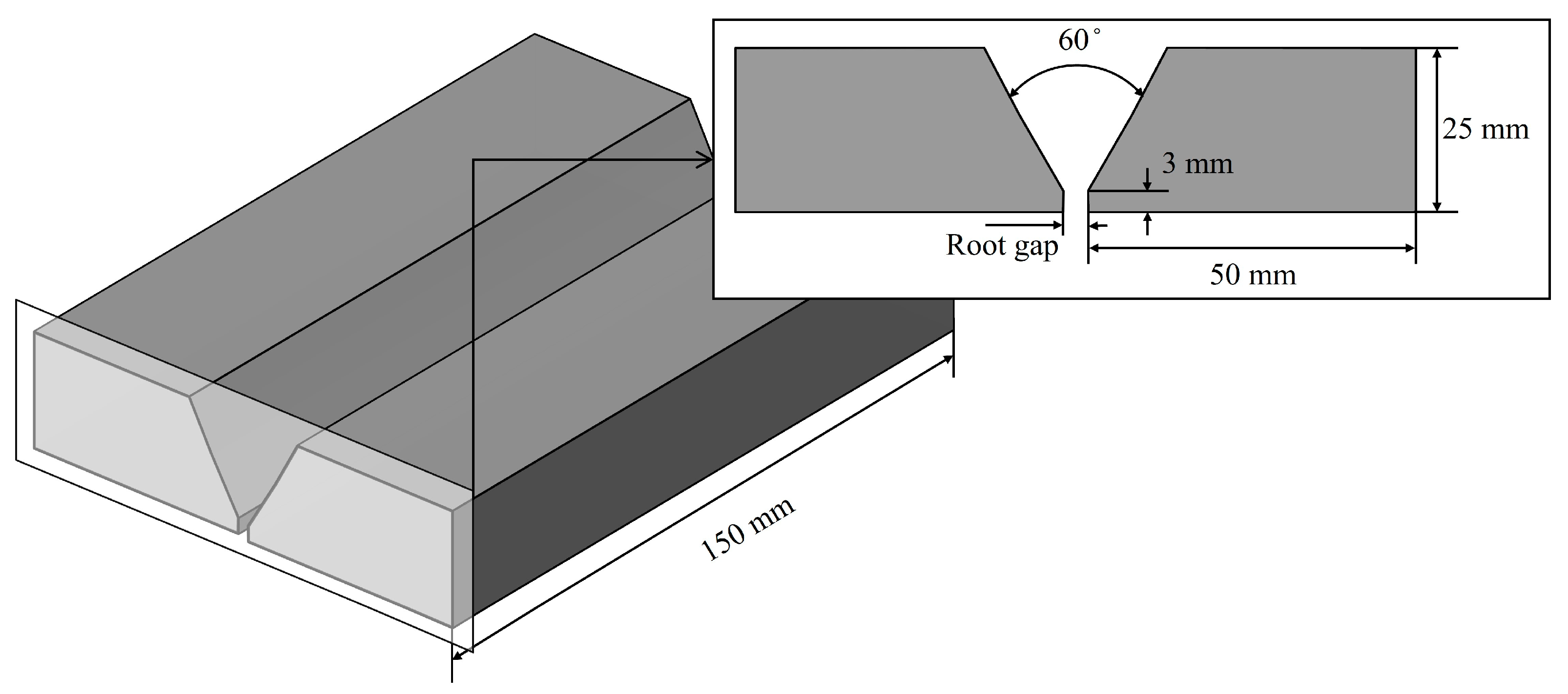
2.1. Joint Shape and Weld Methods

The welding material used was SM 490 with a thickness of 25 mm, and the welding joint was configured as shown in Figure 1. The welding test pieces consisted of two specimens with dimensions of 50 mm × 25 mm × 150 mm, selected with a V-groove configuration for butt welding. The groove angle and root face were set to 60° and 3.0 mm, respectively [11]. The root gap was set to 1.0 mm and 2.0 mm. The welding wire used was AWS A5.18 ER70S-3 1.2 mm, and GMAW was performed on the prepared welding test pieces.

The welding conditions are presented in

Table 1. Welding parameter.

Waveform	DC Pulse
WFR	7.0–12.0 m/min
Welding speed	30 cm/min
CTWD	20 mm
Shielding gas (Flow rate)	90% Ar + 10% CO2 (25 L/min)

. The power source was a Welbee P500L supply (Daihen, Osaka, Japan) that utilizes a direct current (DC) pulse waveform for welding. The wire feed rate (WFR) was varied within 7.0–12.0 m/min and was adjusted to 1.0 m/min level increments, and three welding experiments were conducted for each condition. In addition, the welding speed remained constant at 30 cm/min, the contact tip-to-workpiece distance (CTWD) was set to 20 mm, and the shielding gas—a 90% Ar + 10% CO₂ mixture—maintained a flow rate of 25 L/min.

2.2. Input and Output Data Structuring Method

Current and voltage measurements were acquired during welding. To appropriately structure the input data, the measurement system and its positions were set as shown in Figure 2. Current and voltage measurements were performed for 30 s at 10 kHz by using a data acquisition (DAQ) module comprising a CompactDAQ chassis (cDAQ-9174, National Instruments, Austin, TX, USA) and analog input module (NI-9229, National Instruments). The current was measured on the ground cable, whereas the voltage was measured between the contact tip and the welded material. The measured current and voltage data were transformed into corresponding dynamic resistance values and processed using STFT, serving as input variables for the CNN model.

Figure 3 illustrates the method used to measure the penetration condition, which is utilized as output data. A laser vision sensor was used to scan the bottom side of the welded specimens. Based on the scanned results, the classes were categorized. The height (h) of the weld bead on the underside of the completed weld specimens was measured using a developed laser vision sensor to obtain the output data. A laser vision sensor with a resolution of 0.02 mm along the X- and Z-axes was utilized. Considering the integrity of the back-bead, h values equal to or greater than 0.2 mm were classified as CJP. The laser sensor was moved along the Y-axis at a speed of 7 mm/s, and h was measured 100 times/s. h values below 0.2 mm were classified as class 0 (PJP), h values equal to or above 0.2 mm were classified as class 1 (CJP), and burn-through instances were classified as class 2. These classes were used as the output data.

2.3. CNN-Based Learning Model for Classification of Penetration Condition

A CNN model was applied to predict the penetration condition in the GMA root-pass weld of a V-groove. CNN, a deep learning model, is primarily used for processing image data. The CNN model extracts features from images and learns using the obtained feature maps. Feature maps are generated through operations utilizing kernels with weights, a process known as convolution. The layers where convolution takes place are called convolution layers. Additionally, pooling is employed to emphasize the data in the feature maps, and the layers where pooling occurs are referred to as pooling layers.

The CNN model for predicting the penetration condition utilized a supervised learning classification model and was constructed using three convolution layers and two pooling layers. The rationale for choosing three convolution layers and two pooling layers was based on several considerations. First, the depth of the network was designed to be sufficient to capture complex patterns in the input data without overfitting. Three convolution layers allow the model to extract low-level, mid-level, and high-level features progressively. The pooling layers, placed after the first and second convolution layers, serve to reduce the spatial dimensions of the feature maps, thereby decreasing the number of parameters and computational load while retaining the most salient information. The convolutional layers and pooling layers were optimized using the Keras Tuner library. Supervised learning is as method where the model is trained using pre-labeled input variables and then makes predictions on new data. Classification models are used when the predicted output is a discrete value.

The current and voltage data during welding were converted into dynamic resistance values to predict the penetration state during the root pass of the V-groove butt joint. The current and voltage during welding were converted into a dynamic resistance, which was then transformed into STFT-formatted image data and utilized as input data. The back-bead was measured using a laser vision sensor, categorized into classes based on height, and used as output data. A total of 2000 data points were randomly selected and divided into a 60% training set (1200 points), a 20% validation set (400 points), and a 20% test set (400 points). The selected input and output data were used to train a CNN model to predict and classify penetration conditions.

3. Results and Discussion

3.1. Input/Output Data for Prediction of Penetration Condition

Figure 4 depicts a schematic of the changes in the state of the back-bead with respect to variations in the WFR and root gap. At a 1.0-mm gap, PJP (class 0) occurred with WFRs ranging from 7.0 to 1.0 m/min, while a CJP (class 1) was achieved at a WFR of 11.0 m/min. At a WFR of 12.0 m/min, burn-through (class 2) occurred without back-bead formation. At a 2.0 mm gap, PJP (class 0) occurred at a WFR of 7.0 m/min. In addition, for WFR values ranging from 8.0 to 9.0 m/min, a mixture of PJP (class 0) and CJP (class 1) was observed. For WFR values ranging from 10.0 to 11.0 m/min, CJP (class 1) was achieved. However, for a WFR of 12.0 m/min, burn-through (class 2) occurred (Figure 4a). Figure 4b shows the cross-sectional shape of the weld joint when PJP, CJP, and burn-through occurred.

Figure 5 illustrates the current and voltage waveforms during welding performed using a DC pulse. The current and voltage waveforms were analyzed to assess the validity of structuring the input data before their composition. The average welding current/voltage and pulse cycle were verified. The average peak current (I_P), average base current (I_B), duration of the peak current (T_IP), and duration of the base current (T_IB) were determined from the current waveform. The average peak voltage (V_P), average base voltage (V_B), duration of the peak voltage (T_VP), and duration of the base voltage (T_VB) were determined from the voltage waveform.

Table 2. Welding current/voltage analysis results according to WFR changes.

WFR (m/min)		7.0	8.0	9.0	10.0	11.0	12.0
Average (A/V)		212/26.4	241/27.4	267/28.1	289/29.2	314/29.8	351/31.1
Pulse cycle (ms)		5.77	5.12	4.79	4.46	4.13	3.85
Current	IP (A)	466	465	464	465	463	466
	IB (A)	36	38	43	47	55	65
	TIP (ms)	1.79	1.77	1.78	1.78	1.76	1.80
	TIB (ms)	2.14	1.67	1.09	0.92	0.36	0.12
Voltage	VP (V)	33.2	34.0	34.3	33.6	33.8	34.2
	Vb (V)	20.8	21.2	21.6	21.5	22.6	22.9
	TVP (ms)	1.60	1.62	1.58	1.61	1.62	1.57
	TVB (ms)	3.33	2.81	2.22	1.94	1.44	1.21

summarizes the analysis of the welding current/voltage waveform with respect to variations in the WFR. The analysis was performed solely in instances where CJP occurred to examine the variations in the welding current/voltage with respect to the WFR. The root gap was maintained at 3.0 mm to induce CJP even at a lower WFR, and a ceramic backing tape was attached to the back of the specimens to prevent burn-through. An increase in the WFR resulted in an increase in the average current/voltage and a decrease in the pulse cycle. From the analysis of the current waveform, as the WFR increased from 7.0 to 12.0 m/min, the peak current I_P and its duration T_IP remained almost constant at 465 A and 1.77 ms, respectively. In contrast, the base current I_B increased from 36 to 65 A, whereas its duration T_IB decreased from 2.14 to 0.12 ms. The voltage waveform, which is dependent on the current waveform, exhibits a similar trend. The peak voltage V_P and its duration T_VP were similar, measuring 33.9 V and 1.60 ms, respectively. V_b exhibits an increasing trend, whereas T_VB shows a decreasing trend. The peak term remained relatively consistent as the WFR changed. However, variations in the pulse cycle and base term indicate that there are differences in the calculated dynamic resistance, highlighting their potential as input data through STFT transformation.

During the welding experiments in this study, at a gap of 0.2 mm and WFR values of 8.0 and 9.0 m/min, a region was observed (Figure 4a) where PJP and CJP coexisted. Under the same welding conditions, PJP and CJP mixtures were formed, prompting the need to examine variations in the welding current/voltage owing to these phenomena. Figure 6 illustrates the welding process conducted at a root gap of 3.0 mm with a WFR of 9.0 m/min. The welding phenomena were captured using a high-speed camera while simultaneously measuring the welding waveform. The average current/voltage for PJP (class 1) and CJP (class 2) were 265 A/28.7 V and 269 A/29.6 V, respectively. Moreover, in the burn-through group (class 3), it was measured as 265 A/31.0 V. For the same WFR, the average current remained consistent with variations in penetration; however, there were fluctuations in the average voltage. The length from the nozzle tip to the arc initiation point is defined as the wire extension (Figure 6a), which was then examined with respect to the form of penetration. It was observed that the wire extension varied based on the form of penetration: 12.0 mm for class 1, 14.5 mm for class 2, and 16.1 mm for class 3. With a constant wire diameter of 1.2 mm, the dynamic resistance during welding increased as the wire extension increased. In the case of a constant-current DC pulse, the extended wire extension increased the welding voltage. Variations in voltage are expected to induce changes in the STFT of the dynamic resistance utilized as input data. In addition, anomalies in the abnormal voltage appeared in the base voltage owing to arcing phenomena in the CJP and burn-through. These occurrences are also expected to reflect changes in the STFT of the dynamic resistance.

3.2. Data Processing and Classification

The solid at the wire end transitions into a liquid because of the arc heat and moves toward the workpiece. As the droplet and workpiece melt under heat from the arc, a molten pool begins to form. Owing to the set welding speed, the molten pool appeared to move in the direction opposite to that of welding. The depth of the molten pool is greatest at a point in time from the moment of melting [29,30,31]. Zong et al. [32] defined the concave region formed by the arc pressure in the molten pool behavior as the gouging region and simulated its size. The gouging region’s length, width, and depth increased linearly, reaching 90% of the quasi-stable state at 0.4 s. The maximum penetration depth was considered when the gouging region had solidified. In this study, when converting current and voltage into STFT of dynamic resistance, we adopted a window size of 0.4 s (Figure 7a). Figure 7a illustrates the dynamic resistance derived from the measured current and voltage during welding with a WFR of 7.0 m/min at a 2.0 mm gap. The selected window size was transformed into an STFT to utilize the dynamic resistance as the input data for the CNN (Figure 7b). The dynamic resistance waveform transformed by STFT was initially 875 × 656 pixels, which was then reduced to 175 × 131 pixels, considering the computational speed of the CNN model. As shown in Figure 7a, the laser vision sensor observes the shape of the back-bead surface. CJP occurred, and according to the classification method defined in the output data, it was classified as Class 1.

3.3. CNN-Based Prediction Model for Classification of Penetration Condition

3.3.1. CNN Model for Predicting Penetration Condition

A CNN model was developed to predict the penetration conditions by converting the welding current/voltage into dynamic resistance. Figure 8 and

Table 3. CNN layer information.

Layer	Type	Parameter	Number of Parameters	Arguments
0	Input	175 × 131
1	Conv2D_1	173 × 129	896	Filter = 32, Size = 3 × 3, Stride = 1, Activation function = ReLU
2	Max_pooling2D_1	86 × 64		Filter = 32, Size = 2 × 2, Stride = 2
3	Conv2D_2	84 × 62	18,496	Filter = 64, Size = 3 × 3, Stride = 1, Activation function = ReLU
4	Max_pooling2D_2	42 × 31		Filter = 64, Size = 2 × 2, Stride = 2
5	Conv2D_3	40 × 29	73,856	Filter = 128, Size = 3 × 3, Stride = 1, Activation function = ReLU
6	Flatten	148,480
7	Dense_1	128	19,005,568	Activation function = ReLU
8	Dropout	128		Probability = 0.3
9	Dense_2	3	387	Activation function = Softmax

depict the model for predicting the penetration condition classification from the dynamic resistance transformed using the STFT. We obtained a random set of 2000 data points, which was divided into a training set of 60% (1200 points), a validation set of 20% (400 points), and a test set of 20% (400 points). The classified dynamic resistance information in the STFT was utilized as the input variable for the operations. The CNN model comprises three convolutional layers and two pooling layers. In the convolutional layers, a kernel size of 3 × 3 pixels and a stride of 1 pixel were selected. The kernel size has to be selected to balance computational efficiency and feature extraction capabilities. Smaller kernels reduce the number of network parameters, lowering computational load and mitigating the risk of overfitting. We determined that a 3 × 3-pixel kernel size is optimal for the model through preliminary testing and evaluation based on prediction accuracy. ReLU and Softmax activation functions were used, and dropout was applied to some parts of the CNN at a rate of 30% to prevent overfitting between the two functions; the CNN model was trained for 50 epochs. Adam was used as the function for model optimization, whereas cross-entropy was employed as the loss function to obtain the difference between the predicted and actual values. Finally, the performance of the model was evaluated using accuracy as a metric to assess its performance.

3.3.2. Evaluation of CNN Model Training

After conducting classification training with 2000 randomly extracted penetration condition data points, the accuracy and loss of the training data were 0.9593 and 0.1036, respectively. The accuracy and loss of the validation data are 0.9516 and 0.1140, respectively. Figure 9 illustrates the training process for the training and validation datasets. The accuracy showed an increasing trend as the training progressed, converging closer to 1. Moreover, the loss gradually converged toward zero as the number of training iterations increased, indicating that the model did not overfit.

The test data can be evaluated using the information from the confusion matrix in Figure 10, which includes the accuracy, precision, recall, and F₁-score, as presented in

Table 4. Learning performance of back-bead prediction CNN model.

Class	Accuracy (%)	Precision (%)	Recall (%)	F1-Score (%)
0	97.8	100	100	100
1		96.2	100	98.1
2		100	86.3	92.7

. Accuracy represents the proportion of correctly predicted instances out of the total data; in this model, the accuracy was 97.7%. Of the 400 test data points, prediction errors occurred for nine data points at the boundary where the actual CJP and burn-through events were observed. Precision measures the proportion of true-positive predictions among all positive predictions made by the classification model. In this case, the precision for class 0, class 1, and class 2 was 100%, 96.2%, and 100%, respectively. Recall represents the proportion of true-positive predictions from all actual positive instances in the dataset. In this context, the recall for class 0, class 1, and class 2 was 100%, 100%, and 86.3%, respectively. The F₁-score, the harmonic means of precision and recall, is particularly critical when evaluating model performance in datasets with imbalanced class distributions. It integrates precision and recall, thus preventing one from compensating for the lack of the other. This balanced performance provides significant advantages when applying the model in real-world settings. In this study, the high F₁-scores indicate that the CNN model not only effectively predicts challenging penetration conditions in V-groove butt welding processes but also handles each class with balanced accuracy. The F₁-score, which is the harmonic means of precision and recall, was 100%, 98.1%, and 92.7%, for class 0, class 1, and class 3, respectively. The CNN model developed in this study is suitable for predicting the penetration conditions in GMAW for V-groove butt joints with gaps ranging from 1.0 to 2.0 mm based on accuracy, precision, recall, and F₁-score. However, if the gap size falls outside the proposed range or if there are changes in the welding process, such as using a flux-cored arc wire, additional data collection and model validation will be necessary.

4. Conclusions

In this study, a CNN model was developed to predict the penetration conditions in the butt welding processes at the root pass of V-groove joints. The following conclusions were drawn:

(1)

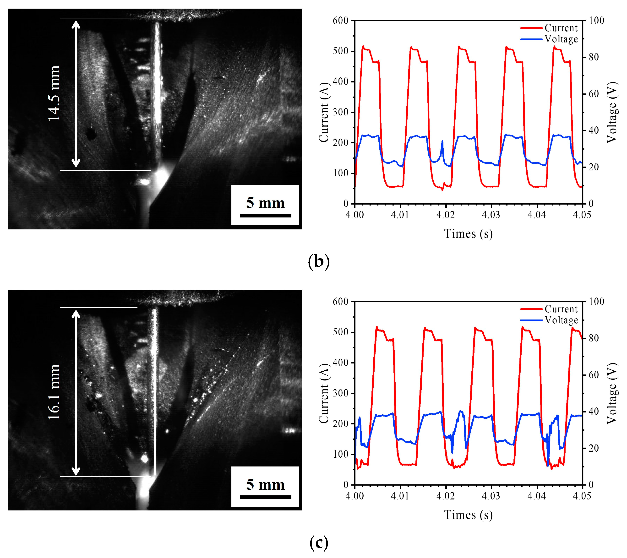
In root-pass welding, penetration conditions such as PJP, CJP, and burn-through were observed. The high-speed camera footage confirmed that as the penetration condition changed, the wire extension length also varied. Consequently, changes in the welding voltage were observed.

(2)

The current and voltage were measured for 30 s at 10 kHz. A window size of 0.4 s was set, considering the deepest position of the weld pool. The STFT of dynamic resistance for this 0.4-s window was utilized as an input variable for the CNN model.

(3)

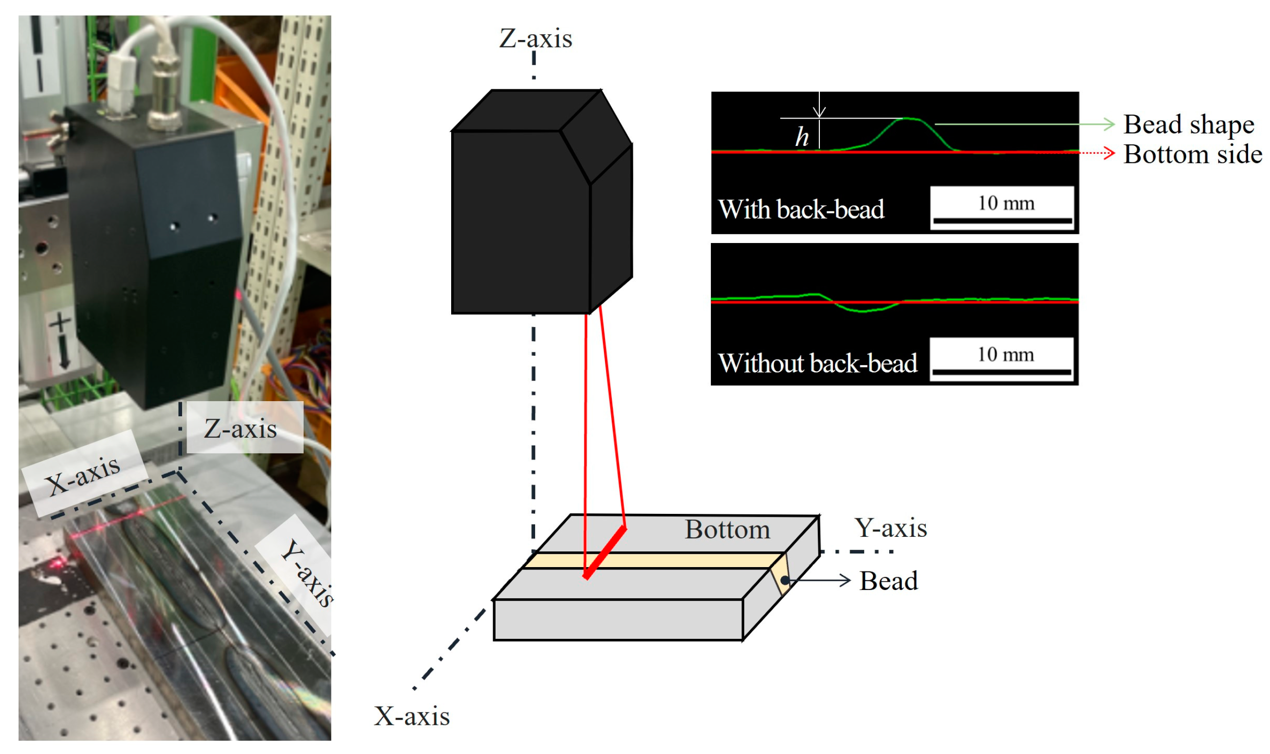
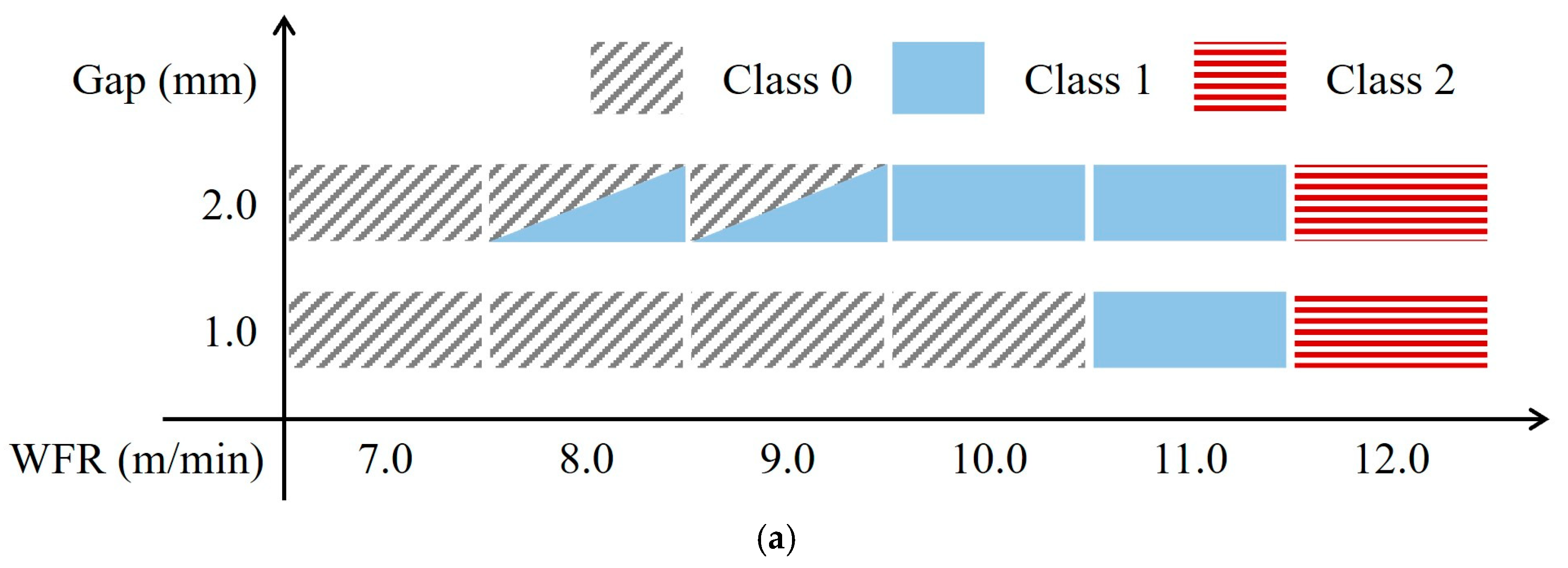
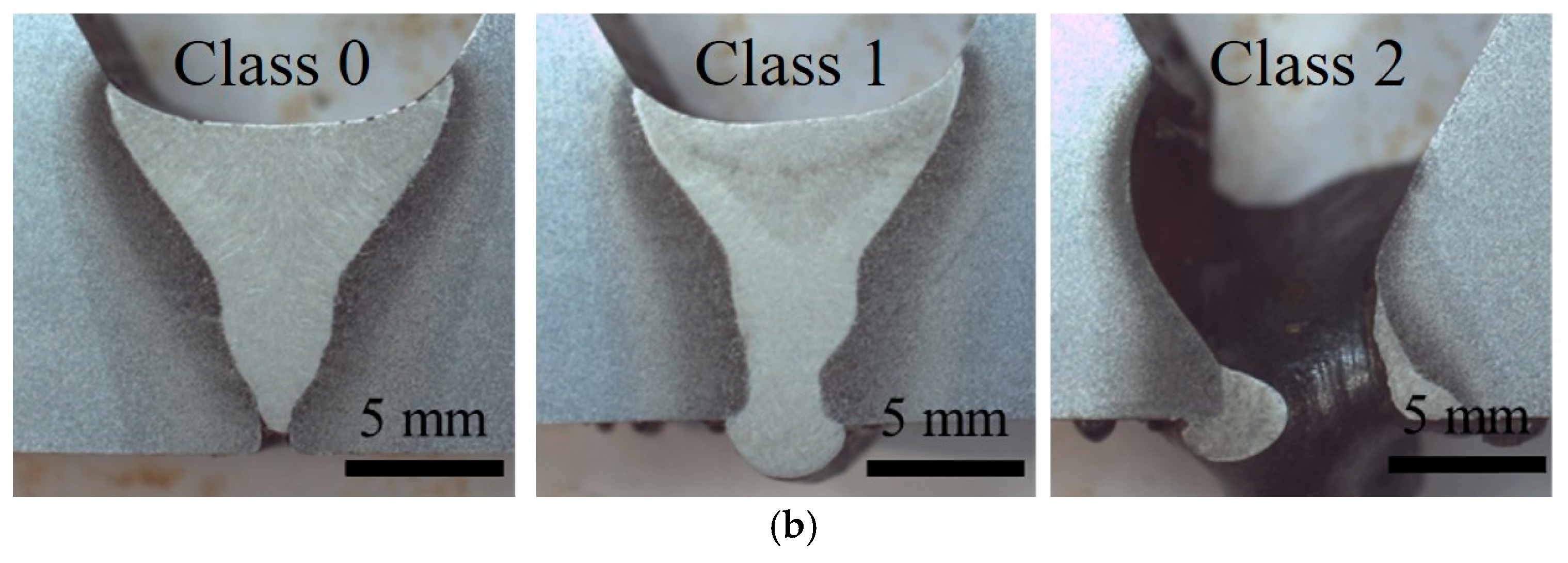
The bottom side of the test piece was scanned using a laser vision system after the welding was completed. Based on the back-bead appearance profile, PJP was classified as class 0, CJP as class 1, and burn-through as class 2; these were used as output variables for the CNN model.

(4)

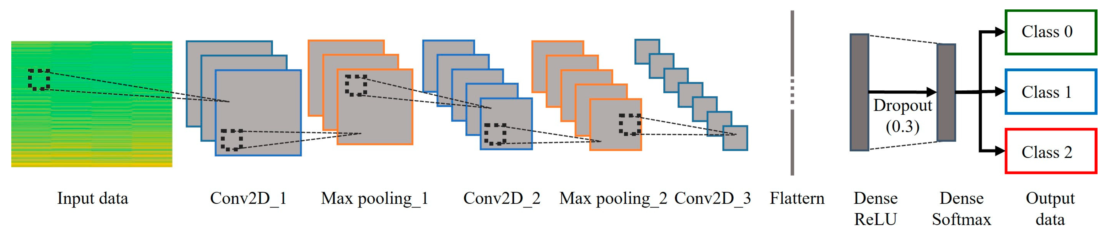
The size of the dynamic resistance STFT was adjusted to enhance the computational speed of the CNN model. A CNN model consisting of three convolutional layers and two pooling layers was adopted, and classification training was performed on the input variables.

(5)

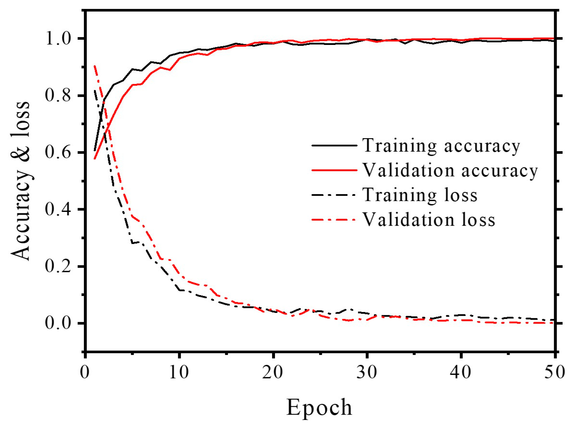
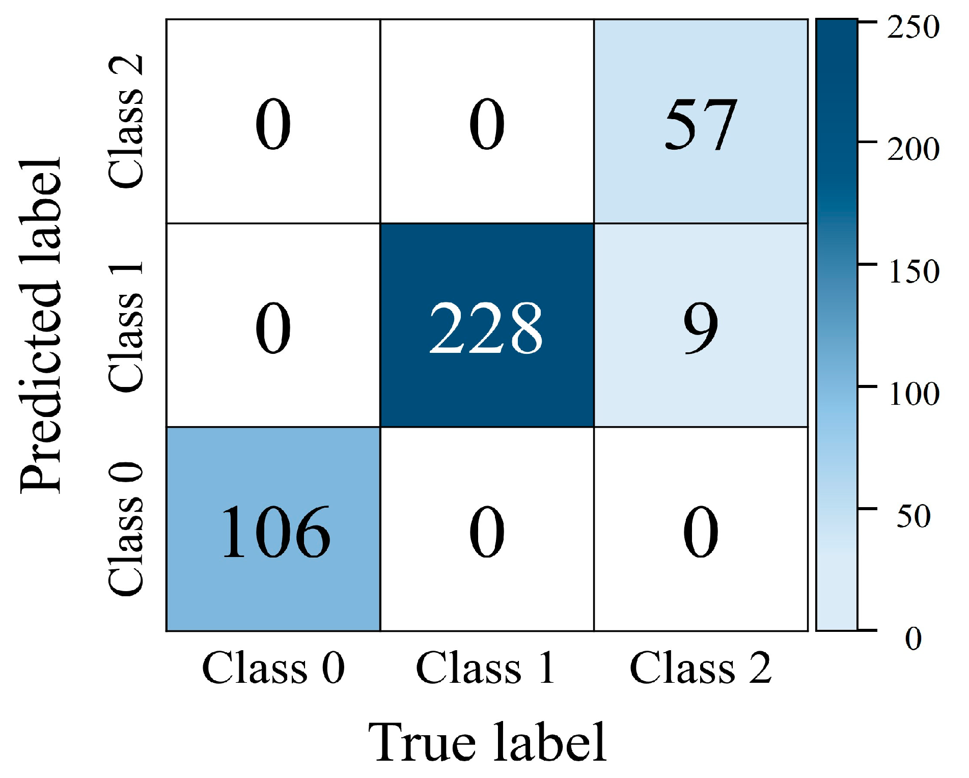
The CNN model achieved a prediction accuracy of 97.7% in predicting the occurrence of penetration conditions in weld joints. For precision, it was 100% for class 0 and class 2, and 96.2% for class 1. For recall, it was 100% for class 0 and class 1 and 86.3% for class 2. For the F₁-score, it was 100% for class 0, 98.1% for class 1 and 92.7% for class 2. The developed CNN model was evaluated as a suitable model for the prediction of the occurrence of penetration conditions in weld joints and welding conditions.

The validation process confirmed that the dynamic resistance STFTs extracted from the welding current and voltage waveforms in this study could be used to determine the penetration conditions. Moreover, it is anticipated that the real-time prediction of the penetration condition can be achieved using the transformed dynamic resistance STFT.

In the future, real-time prediction will be necessary for determining penetration conditions. We plan to identify the key feature points of dynamic resistance related to penetration conditions. Additionally, we aim to develop an ANN model with a faster computation speed than the CNN model.

References

1. Chen, T.; Xue, S.; Wang, B.; Zhai, P.; Long, W. Study on short-circuiting GMAW pool behavior and microstructure of the weld with different waveform control methods. Metals 2019, 9, 1326. [Google Scholar] [CrossRef]
2. Shen, X.; Ma, G.; Chen, P. Effect of welding process parameters on hybrid GMAW-GTAW welding process of AZ31B magnesium alloy. Int. J. Adv. Manuf. Technol. 2018, 94, 2811–2819. [Google Scholar] [CrossRef]
3. Wu, K.; Ding, N.; Yin, T.; Zeng, M.; Liang, Z. Effects of single and double pulses on microstructure and mechanical properties of weld joints during high-power double-wire GMAW. J. Manuf. Process. 2018, 35, 728–734. [Google Scholar] [CrossRef]
4. Ikram, A.; Chung, H. The effect of EN ratio and current on microstructural and mechanical properties of weld joined by AC-GMAW on square groove butt joints. Appl. Sci. 2017, 7, 261. [Google Scholar] [CrossRef]
5. Su, L.; Fei, Z.; Davis, B.; Li, H.; Bornstein, H. Digital image correlation study on tensile properties of high strength quenched and tempered steel weld joints prepared by K-TIG and GMAW. Mate. Sci. Eng. A 2021, 827, 142033. [Google Scholar] [CrossRef]
6. Datta, R.; Mukerjee, D.; Rohira, K.L.; Veeraraghavan, R. Weldability evaluation of high tensile plates using GMAW process. J. Mater. Eng. Perform. 1999, 8, 455–462. [Google Scholar] [CrossRef]
7. Kim, D.Y.; Kim, G.G.; Yu, J.; Kim, D.; Kim, Y.M.; Park, J. Improvement of fatigue performance by applying tandem GMAW in lap joints with gaps. Int. J. Adv. Manuf. Technol. 2023, 128, 2123–2135. [Google Scholar] [CrossRef]
8. Svoboda, H.G.; Nadale, H.C. Fatigue life of GMAW and PAW welding joints of boron microalloyed steels. Procedia Mater. Sci. 2015, 9, 419–427. [Google Scholar] [CrossRef]
9. Kim, D.Y.; Hwang, I.; Jeong, G.; Kang, M.; Kim, D.; Seo, J.; Kim, Y.M. Effect of porosity on the fatigue behavior of gas metal arc welding lap fillet joint in GA 590 MPa steel sheets. Metals 2018, 8, 241. [Google Scholar] [CrossRef]
10. Kim, D.Y.; Kim, G.G.; Yu, J.; Kim, D.; Kim, Y.M.; Park, J. Weld fatigue behavior of gas metal arc welded steel sheets based on porosity and gap size. Int. J. Adv. Manuf. Technol. 2023, 124, 1141–1153. [Google Scholar] [CrossRef]
11. AWS D1.1/D1.1M; Structural Welding Code—Steel. American Welding Society: Miami, FL, USA, 2020.
12. EN ISO 5817: 2006-10; Welding—Fusion-Welded Joints in Steel, Nickel, Titanium and Their Alloys (Beam Welding Excluded)—Quality Levels for Imperfections. ISO: Geneva, Switzerland, 2006.
13. Pradhan, R.; Joshi, A.P.; Sunny, M.R.; Sarkar, A. Performance of predictive models to determine weld bead shape parameters for shielded gas metal arc welded T-joints. Mar. Struct. 2022, 86, 103290. [Google Scholar] [CrossRef]
14. Nagesh, D.S.; Datta, G.L. Genetic algorithm for optimization of welding variables for height to width ratio and application of ANN for prediction of bead geometry for TIG welding process. Appl. Soft. Comput. 2010, 10, 897–907. [Google Scholar] [CrossRef]
15. Sarkar, A.; Dey, P.; Rai, R.N.; Saha, S.C. A comparative study of multiple regression analysis and back propagation neural network approaches on plain carbon steel in submerged-arc welding. Sādhanā 2016, 41, 549–559. [Google Scholar] [CrossRef]
16. Xu, W.H.; Lin, S.B.; Fan, C.L.; Yang, C.L. Prediction and optimization of weld bead geometry in oscillating arc narrow gap all-position GMA welding. Int. J. Adv. Manuf. Technol. 2015, 79, 183–196. [Google Scholar] [CrossRef]
17. Abioye, T.E.; Mustar, N.; Zuhailawati, H.; Suhaina, I. Prediction of the tensile strength of aluminium alloy 5052-H32 fibre laser weldments using regression analysis. Int. J. Adv. Manuf. Technol. 2019, 102, 1951–1962. [Google Scholar] [CrossRef]
18. Achebo, J.I.; Eki, M.U. Prediction of mild steel weld properties using artificial neural network and regression analysis. Trop. Technol. J. 2020, 1, 37–49. [Google Scholar] [CrossRef]
19. Jung, J.S.; Lee, H.K.; Park, Y.H. Prediction of tensile strength for Plasma-MIG hybrid welding using statistical regression model and neural network algorithm. J. Weld. Join. 2016, 34, 67–72. [Google Scholar] [CrossRef]
20. Kim, D.Y.; Hwang, J.H.; Kim, G.G.; Kim, Y.M.; Yu, J.; Park, J. Prediction of weld tensile-shear strength using ANN based on the weld shape in Aluminum alloy GMAW. J. Weld. Join. 2023, 41, 17–27. [Google Scholar] [CrossRef]
21. Alvarez Bestard, G.; Absi Alfaro, S.C. Measurement and estimation of the weld bead geometry in arc welding processes: The last 50 years of development. J. Braz. Soc. Mech. Sci. Eng. 2018, 40, 444. [Google Scholar] [CrossRef]
22. Yu, R.; Zhao, Z.; Bai, L.; Han, J. Prediction of weld reinforcement based on vision sensing in GMA additive manufacturing process. Metals 2020, 10, 1041. [Google Scholar] [CrossRef]
23. Dong, H.; Cong, M.; Zhang, Y.; Liu, Y.; Chen, H. Modeling and real-time prediction for complex welding process based on weld pool. Int. J. Adv. Manuf. Technol. 2018, 96, 2495–2508. [Google Scholar] [CrossRef]
24. Jiao, W.; Wang, Q.; Cheng, Y.; Zhang, Y. End-to-end prediction of weld penetration: A deep learning and transfer learning based method. J. Manuf. Process. 2021, 63, 191–197. [Google Scholar] [CrossRef]
25. Liang, R.; Yu, R.; Luo, Y.; Zhang, Y. Machine learning of weld joint penetration from weld pool surface using support vector regression. J. Manuf. Process. 2019, 41, 23–28. [Google Scholar] [CrossRef]
26. Lu, J.; Shi, Y.; Bai, L.; Zhao, Z.; Han, J. Collaborative and quantitative prediction for reinforcement and penetration depth of weld bead based on molten pool image and deep residual network. IEEE Access 2020, 8, 126138–126148. [Google Scholar] [CrossRef]
27. Pal, S.; Pal, S.K.; Samantaray, A.K. Neurowavelet packet analysis based on current signature for weld joint strength prediction in pulsed metal inert gas welding process. Sci. Technol. Weld. Join. 2008, 13, 638–645. [Google Scholar] [CrossRef]
28. Pal, S.; Pal, S.K.; Samantaray, A.K. Sensor based weld bead geometry prediction in pulsed metal inert gas welding process through artificial neural networks. Int. J. Knowl.-Based Intell. Eng. Syst. 2008, 12, 101–114. [Google Scholar] [CrossRef]
29. Jeong, H.; Park, K.; Baek, S.; Kim, D.Y.; Kang, M.J.; Cho, J. Three-dimensional numerical analysis of weld pool in GMAW with fillet joint. J. Precis. Eng. Manuf. 2018, 19, 1171–1177. [Google Scholar] [CrossRef]
30. Hu, Z.; Hua, L.; Qin, X.; Ni, M.; Ji, F.; Wu, M. Molten pool behaviors and forming appearance of robotic GMAW on complex surface with various welding positions. J. Manuf. Process. 2021, 64, 1359–1376. [Google Scholar] [CrossRef]
31. Cho, D.W.; Park, J.H.; Moon, H.S. A study on molten pool behavior in the one pulse one drop GMAW process using computational fluid dynamics. Int. J. Heat Mass Transf. 2019, 139, 848–859. [Google Scholar] [CrossRef]
32. Zong, R.; Chen, J.; Wu, C.; Lou, D. Numerical analysis of molten metal behavior and undercut formation in high-speed GMAW. J. Mater. Process. Technol. 2021, 297, 117266. [Google Scholar] [CrossRef]
Figure 1. Configuration of butt joint.
Applsci 14 04883 g001
Figure 2. Welding current and voltage measurement system and measurement methodology.
Applsci 14 04883 g002
Figure 3. Back-bead measurement method and output data classification.
Applsci 14 04883 g003
Figure 4. Gap and WFR changes: (a) schematic of penetration-type classification; and (b) cross-section image according to classification.
Applsci 14 04883 g004aApplsci 14 04883 g004b
Figure 5. Schematic of analysis method with welding waveform.
Applsci 14 04883 g005
Figure 6. Welding phenomena images and current/voltage corresponding to varying forms of penetration: (a) PJP (class 1); (b) CJP (class 2); and (c) burn-through (class 3).
Applsci 14 04883 g006aApplsci 14 04883 g006b
Figure 7. Input/output data preprocessing and data classification: (a) convert current/voltage to dynamic resistance and classify output data; and (b) STFT conversion of dynamic resistance data to utilize input data.
Applsci 14 04883 g007
Figure 8. CNN-based back-bead prediction model structure.
Applsci 14 04883 g008
Figure 9. Curve of accuracy and loss.
Applsci 14 04883 g009
Figure 10. Confusion matrix of test dataset.
Applsci 14 04883 g010