Physical Simulation-Based Calibration for Quantitative Real-Time PCR

Abstract

The fluorescence quantitative polymerase chain reaction (qPCR) instrument has been widely used in molecular biology applications, where the reliability of the qPCR performance directly affects the accuracy of its detection results. In this paper, an integrated, physics-based calibration device was developed to improve the accuracy and reliability of qPCR, realizing the calibration of qPCR instruments’ standard curve through physical simulations. With this calibration device, the collected temperature was used as the control signal to alter the fluorescence output, which allowed different probes to simulate the Ct values corresponding to samples with varying initial concentrations. The temperature and optical performance of this calibration device were tested, followed by a comparative analysis comparing the on-machine test results with standard substances to assess the linearity and uniformity of the Ct values of the measured qPCR instrument. It has been proven that this physical calibration device can effectively replace the biochemical standard substance to carry out comprehensive calibration of the temperature and optical parameters of the qPCR instrument and provide a more reliable method for the periodic calibration and quality control of the qPCR instrument. This contributes to the accuracy and reliability of fluorescence qPCR instruments in the field of molecular biology.

1. Introduction

Fluorescence quantitative PCR (qPCR) instruments are utilized for various nucleic acid detection and gene analysis characterized by the polymerase chain reaction (PCR) technique, aimed at detecting DNA/RNA with extensive applications in clinical diagnostics [1,2,3], animal quarantine [4], forensic identification [5], adulteration identification and species identification [6,7,8], in vitro diagnostics [9], and pharmaceutical research and development [10]. Particularly, amidst the global outbreak of the COVID-19 pandemic, qPCR method has emerged as the gold standard [11] for nucleic acid detection, leading to a larger-scale deployment of qPCR instruments in the field of molecular biology. Furthermore, qPCR instruments are also employed in environmental monitoring, such as pathogen monitoring in wastewater [12]. With the extensive applications of qPCR instruments, its users urge a comprehensive performance evaluation of the qPCR. In such evaluation, factors impacting the accuracy of the qPCR instruments results pose a significant challenge to the calibration.

In comparison to qualitative PCR instruments, the factors of qPCR instruments are more intricate. Key factors include the type of chemical reagents, temperature factors of the temperature module and lid, specification of the filters, reflectors and optical path channels, sensitivity of the fluorescence receiver, mechanical components, and threshold settings in software such as baseline and S/N ratio, etc. These factors pose significant challenges for the calibration of qPCR instruments.

Quality control and regular calibration of qPCR instruments are crucial, as they directly impact quantitative results including Ct values, precision, detection limit, and specificity [13]. Two main reasons for influencing the accuracy and repeatability of qPCR instrument results are edge effects and experimental errors. Edge effects are caused by defects in the optical detection system design and the temperature control module, also known as sample tray (Block). Such defects can lead to differences in the optical path lengths between edge wells and central wells of qPCR instrument Block resulting in variations in the excitation light energy received by fluorescent groups in different wells, and ultimately affecting the reliability of experimental results, namely Ct values. Similarly, temperature differences between wells within the Block can also lead to such edge effects with even small optical or temperature differences between wells may be exponentially amplified during the amplification process, ultimately affecting experimental results [14,15].

The structural design of the optical detection system in qPCR instruments can also impact the stability and detection limit of detection [16]. Additionally, defects in the optical path design and differences in inter-well temperatures directly affect the results of melting curve analysis, leading to significant variations in resolution among different instruments. This influence can result in an inability to successfully differentiate mutant genes or misidentification of mutant genes when detecting mutations or performing single nucleotide polymorphism analysis using melting curve analysis. Regular calibration of qPCR instruments helps ensure the reliability and accuracy of the equipment, providing support for traceability and quality control.

In the detection of respiratory pathogens, the Ct value of qPCR reactions is widely used as an epidemiological and clinical indicator [17,18]. The Ct value is negatively correlated with the initial viral load, allowing for indirect quantification of the starting virus copy number [19,20]. Typically, due to variations in reported Ct values from different PCR methods, it is necessary to use a standard curve for accurate quantification of expected virus copy number [21]. The standard curve produced by qPCR is a well-established method for the quantification of nucleic acids [22], in the absence of a gold standard test, the standard curve method is often used to construct and verify the reliability of qPCR instruments for nucleic acid detection [23,24]. Moreover, following the COVID-19 pandemic, the importance of Ct values has been further emphasized, with many studies focusing on exploring the correlation between Ct values and disease severity and transmissibility [25,26], as well as the correlation between Ct values and epidemiological trends [21]. In addition to the content of the tested samples, Ct values are also influenced by factors such as the temperature and optical performance of the qPCR instrument itself [27], the use of reagent kits, sample collection time, primer specificity, amplification efficiency, sample inactivation temperature, and inactivation time [28].

To ensure experimental accuracy, researchers can periodically calibrate specific fluorescence channels of qPCR instruments using fluorescence dyes according to the calibration methods provided by the manufacturer [29]. Additionally, qPCR instrument manufacturers generally recommend using the manufacturer-provided matching ROI calibration plates to calibrate the fluorescence signals. This method allows for the collection of the position and intensity of fluorescence signals in each reaction well, thereby determining whether overexposure or underexposure occurs during detection and subsequent correction. However, this step is typically only used when there are noticeable inaccuracies in instrument performance.

Users are more inclined to comprehensively confirm the performance of qPCR instruments using positive controls, negative controls, gradient dilution quality control samples, or comparing the results with those obtained from reference instruments [30]. In general, fluorescence detection reagents are sourced from the instrument manufacturer or third-party testing institutions. During the reagent formulation process, strict control of the proportions of each substance is necessary, however, human reading errors are unavoidable. For example, when preparing standard substances of different concentrations through gradient dilution of the same batch of reagents, minor errors in pipetting may lead to the reagent standard substance concentration being lower than the expected target concentration, and this error will be continuously introduced into the entire amplification process [12]. Additionally, properly prepared chemical reagents require strict transportation and storage conditions. However, there are many uncontrollable objective errors during transportation to the laboratory being tested which can result in inaccuracies in chemical reagent detection. Moreover, conventional laboratory quality control and calibration standards still predominantly rely on using standard substances to calibrate the sample linearity of the standard curve of qPCR instruments. The calibration indicators of physical devices differ significantly from those of conventional methods, making them difficult to compare and substitute.

In consideration of the recent calibration requirements for PCR instruments, this study proposed a method for temperature-optical calibration of qPCR instruments using a physical method and developed a calibration device based on physical simulation with integrated temperature–fluorescence probes. The calibration device was a PCR amplification simulator that incorporates temperature and standard light sources to synchronize the calibration of the temperature and optical parameters of the PCR instrument. It could calibrate temperature deviation, temperature uniformity, heating and cooling rate, Ct value, melting temperature and other parameters. By controlling the output fluorescence through monitoring temperature collection, different probes could simulate different Ct values corresponding to samples with varying initial concentrations, thus simulating a standard curve using a physical device and calibrating qPCR instruments. The different probes of the device were independently controlled, and a single malfunction did not affect the operation of others. The probes were assembled and fixed in a nested manner, allowing for various arrangement options. The 8-probe unit served as the basic unit, which can be used individually or in combination with multiple units to expand its application for calibration of 8-well, 16-well, 48-well, and 96-well qPCR instruments. Furthermore, this device could perform the functions of other physical calibration devices. It could comprehensively, controllably, and traceably replace standard substances for qPCR instrument calibration, ensuring the accuracy of equipment usage.

2. Principle and Structure

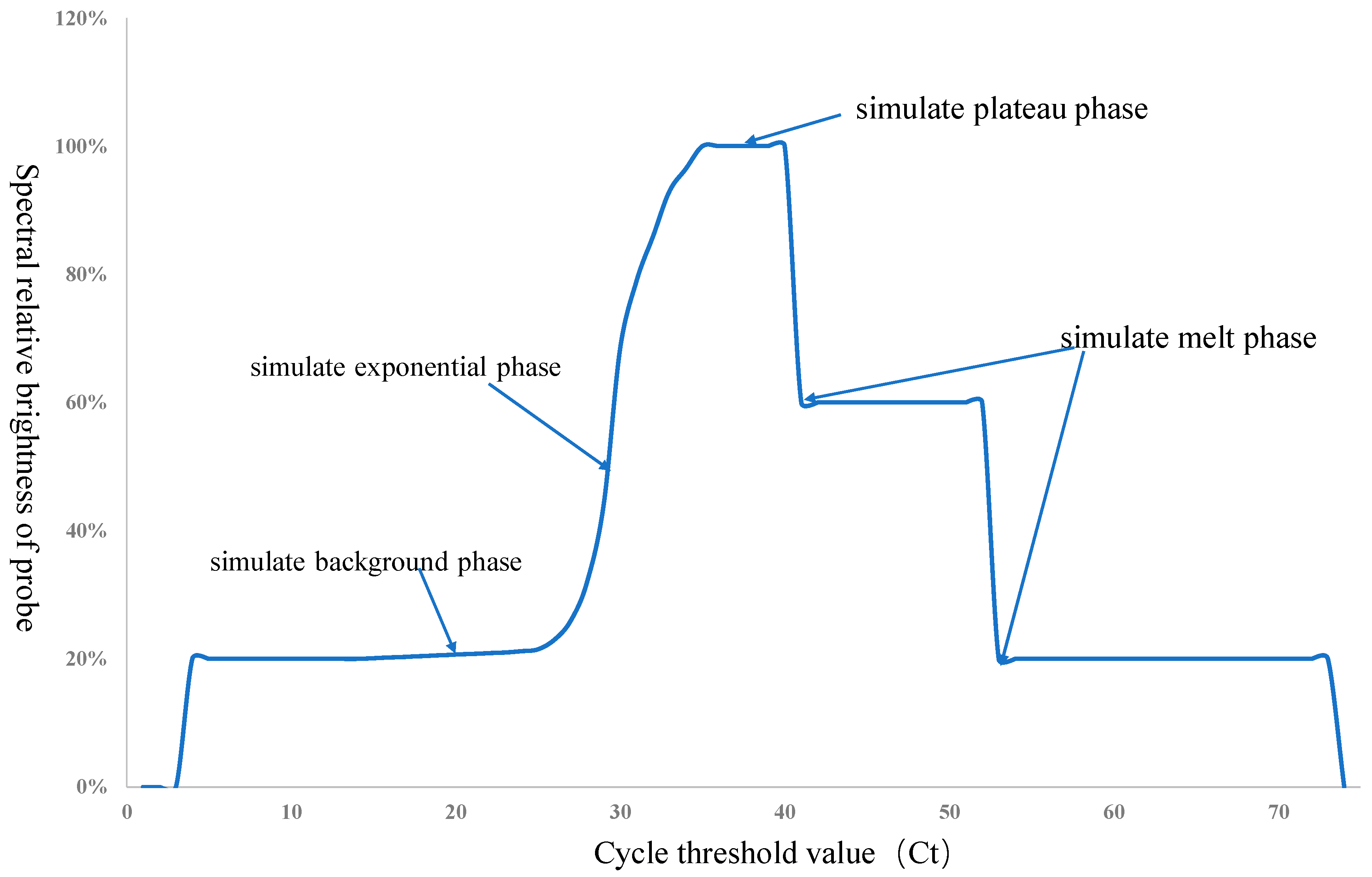
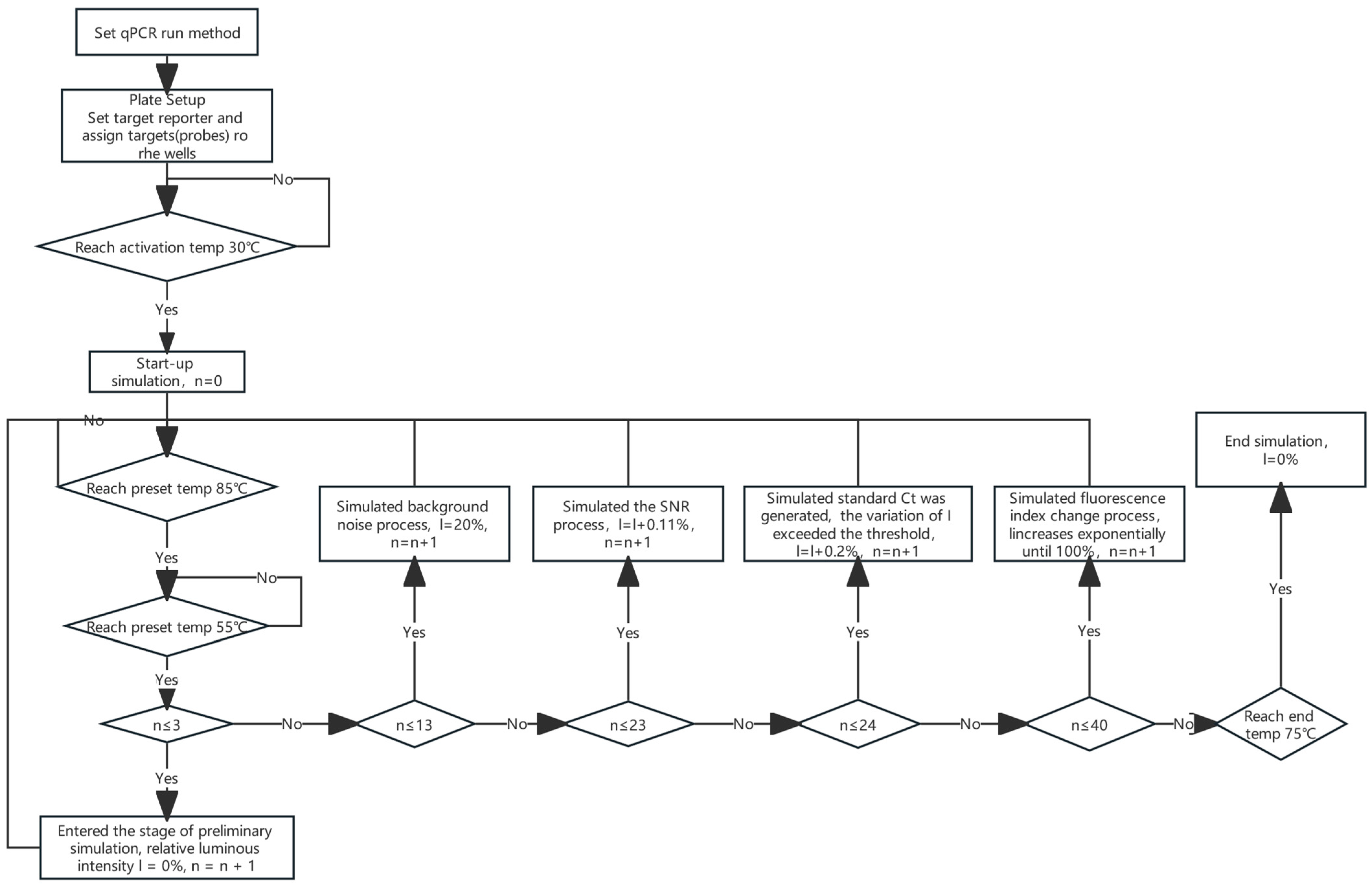
2.1. Principles of Calibration Device

The principle diagram of the developed calibration device is shown in Figure 1. The temperature acquisition module employs a high-precision thermistor encapsulated within a purple copper casing. The fluorescence output module utilizes calibrated light-emitting diodes (LEDs) as standard light sources that are traceable to a spectrometer, encapsulated with polytetrafluoroethylene (PTFE) for optical transparency. These two components are nested together to form a calibration unit, that is, a probe. The outer contour of probes is designed to fit snugly into the inner contour of the porous metal block of qPCR instruments, ensuring an effective fit and accuracy in temperature data collection.

In the device host, the selected ADC for the calibration device features low noise (40 nVrms) and low power consumption (400 μA), along with a relatively high sampling rate. The acquisition module is constructed to connect two sets of ADCs and one set of channel switches. Each set interfaces with four temperature probes, with each probe acquiring data four times to calculate an average value. This allows the calibration device to filter out noise and other similar interferences. Probes numbered 1 to 8 undergo cyclic serial acquisition, facilitating the output of two measurements per second. To enable wireless control and data transmission with computer software, the device employs 2.4 GHz low-power Bluetooth technology as the communication protocol.

The ideal PCR reaction amplification curve should satisfy Equation (1). However, actual PCR reactions are non-ideal and are influenced by various factors such as primers, enzymes, etc., conforming to the description in Equation (2) [20].

$$X_n=X_0\times 2^n$$

(1)

$$X_n=X_0\times {(1+E_n)}^n$$

(2)

$X_n$ represents the amount of amplified product after the nth cycle; $X_0$ denotes the initial template quantity; $E_n$ signifies the amplification efficiency; and $n$ indicates the number of amplification cycles.

According to Equation (2), in actual PCR reactions, a typical amplification process follows an S-shaped curve, including the background phase, exponential amplification phase, and plateau phase. Based on this theory, the calibration device can control the standard light source within the probe based on temperature changes collected by the temperature acquisition module. This control ensures that the light emission intensity changes according to a predefined process, simulating the brightness changes of fluorescence groups during the amplification reaction. The simulated fluorescence is received by the qPCR instrument to mimic a typical amplification curve. The controller of the calibration device drives different electric current levels to the fluorescence output module of probes, resulting in varying intensities of fluorescence brightness. Specifically, during the initial stage, it simulates the background phase by causing only minimal changes in standard light source emission, resulting in growth below a certain threshold. In the second stage, it simulates the exponential amplification phase by causing a fluorescent brightness change that follows an exponential pattern after subtracting background noise. And, during the beginning of this phase, it simulates the pre-set Ct value. This means that when the number of cycles corresponding to this Ct value is reached, the standard light source’s emission undergoes a slight increase just enough to surpass the threshold and be detected by the qPCR instrument. In the third stage, it simulates the plateau phase where standard light source emission gradually reaches 100%. After completing simulation of an S-shaped curve representing amplification, the probe can also be designed to simulate the melting curve process by emulating half DNA denaturation-induced fluorescence and reducing standard light source emission by equal magnitude. The designed simulated fluorescence process is illustrated in Figure 2.

Ct values are inversely correlated with the initial viral load and can indirectly quantify the initial viral copy number [19]. Therefore, by simulating different Ct values for each probe of the calibration device and varying the light emission accordingly, the simulation of a series of diluted standard substance curves can be achieved. When the eight probes of the calibration device simulate different Ct values, each probe only needs to sequentially generate optical changes, as shown in Figure 2, according to the set Ct value steps successively. In order to simulate a Ct value such as 24, the temperature acquisition control process for light emission variation by this probe is illustrated in Figure 3. Additionally, probes can also simulate the fluorescence of negative control by maintaining a constant low level of emission (e.g., I = 20%).

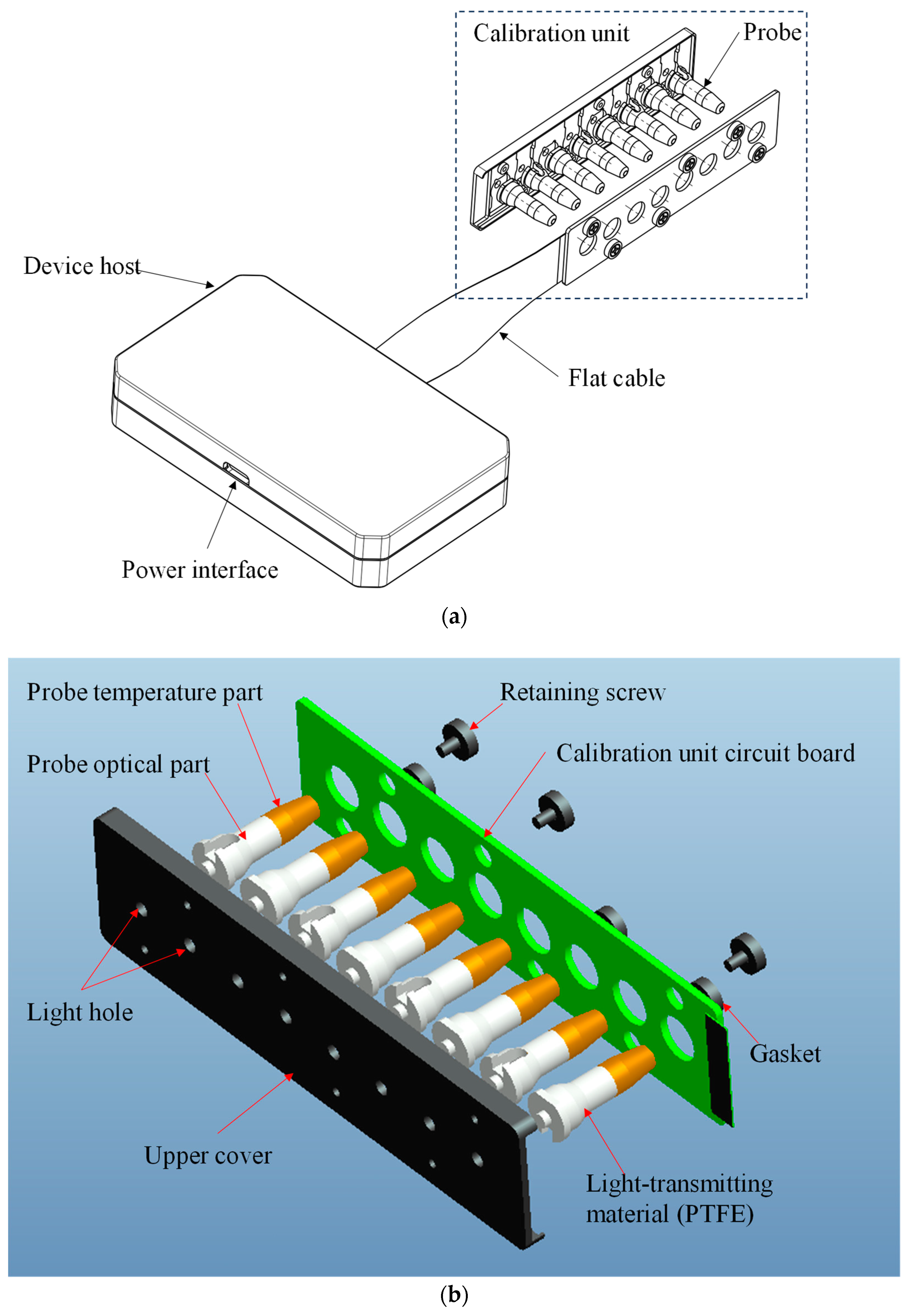
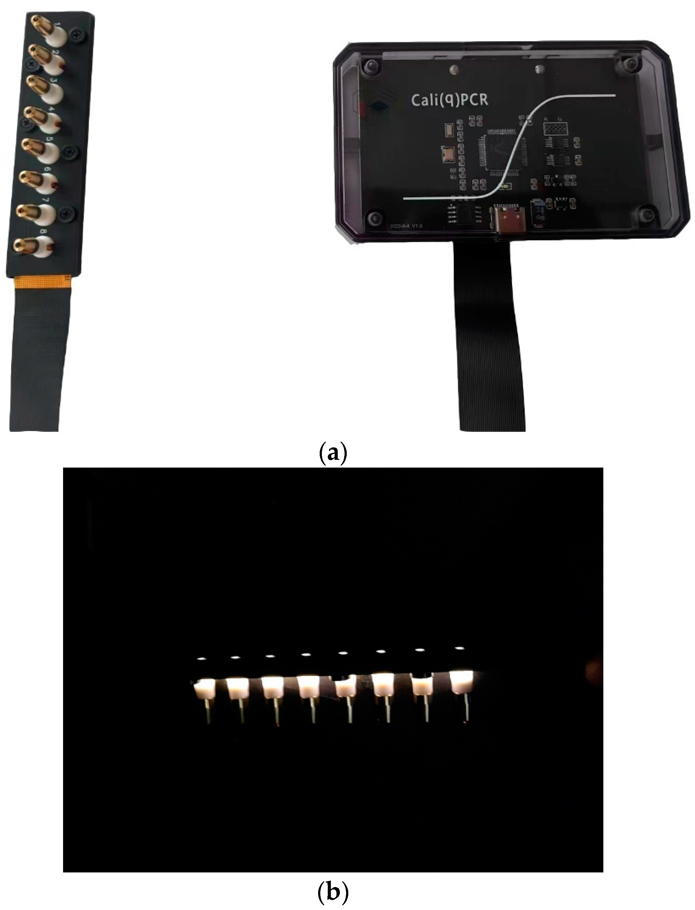
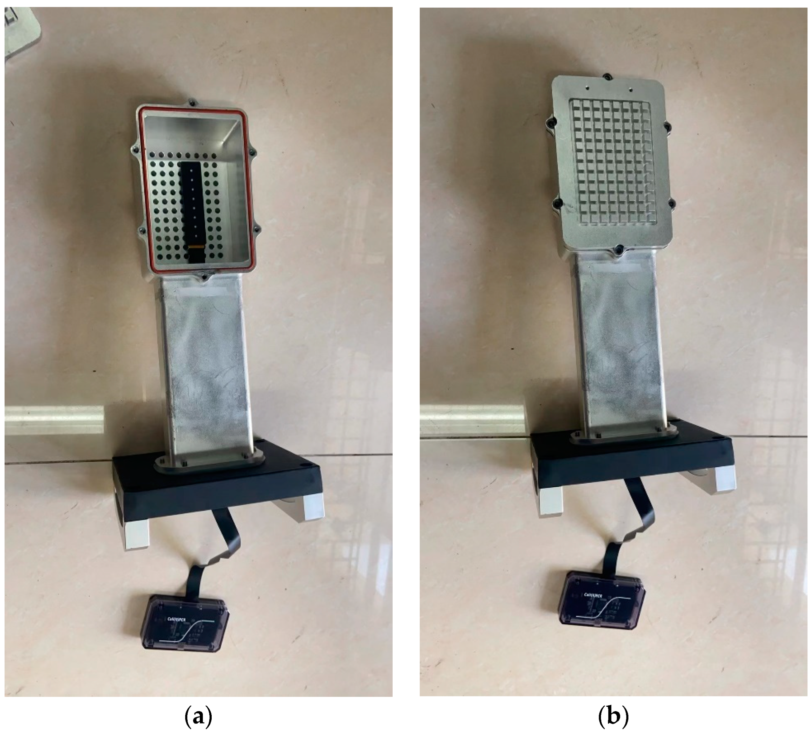
2.2. Structure of the Calibration Device

The structural design of the calibration device is illustrated in Figure 4, comprising a host and calibration units. The calibration unit consists of an upper cover plate, a circuit board, and eight probes.

There are eight 2 mm diameter transparent holes on the upper cover plate, while the bottom plate, i.e., the circuit board, contains through-holes allowing the probes to pass through. The top of probes is designed with irregular nested shapes to fit between the upper cover plate and the bottom plate, ensuring that the light emission position of the standard light source precisely aligns with the translucent point. This alignment guarantees that the emitted light from the standard source can be captured by the qPCR instrument during the actual calibration process, and the collected fluorescence data automatically generate measured amplification curves. The optical part of the probe was machined separately using the PTFE rods and then assembled with the temperature part. The heated top cover plate on the qPCR instrument, typically operating at temperatures between 90 °C to 105 °C, allows the calibration device to continuously operate at high temperatures. To achieve this, the top cover plate undergoes multiple high-temperature aging processes to ensure that it remains unaffected by temperature-induced deformation during actual use. The top cover plate features a hollow design, allowing the protruding components of the circuit board to be embedded within it. The top cover plate and bottom plate are secured by four position screws, effectively reducing the thickness of the calibration device’s substrate and enabling it to accommodate various types of qPCR instrument for detection. The physical appearance of the calibration device is shown in Figure 5.

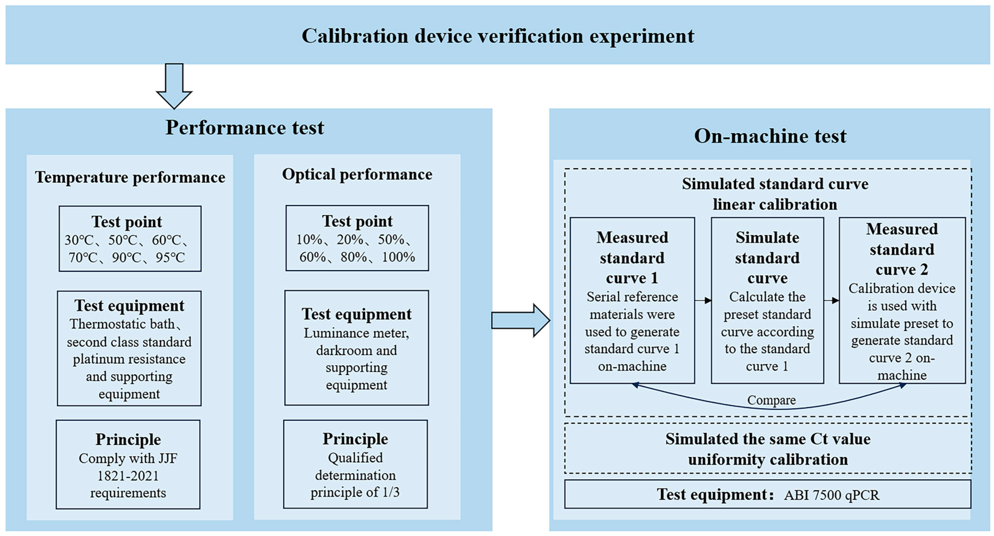
2.3. Experimental Scheme

In this calibration device the optical part uses PTFE, with the expansion coefficient being (25~250 °C) of 10~12 × 10⁻⁵/°C, thermal conductivity being 0.19~0.25 W/m·K, and refractive index being 1.37 (20 °C). The optical part uses 30% glass fiber reinforced poly ether ether ketone (PEEK) with tensile strength being 115 MPa at 125 °C, flexural strength being 190 MPa at 125 °C, and thermal conductivity being 0.35 W/m·K. This paper conducted temperature performance tests and optical performance tests on the developed calibration device, ensuring that its technical specifications meet the requirements for qPCR instrument calibration. Subsequently, on-machine tests are employed to validate the feasibility of the calibration device’s simulation of standard curves for implementing linear calibration schemes on qPCR instruments, along with its applicability for calibrating uniformity of qPCR instruments. The experimental design is illustrated in Figure 6.

3. Performance Test

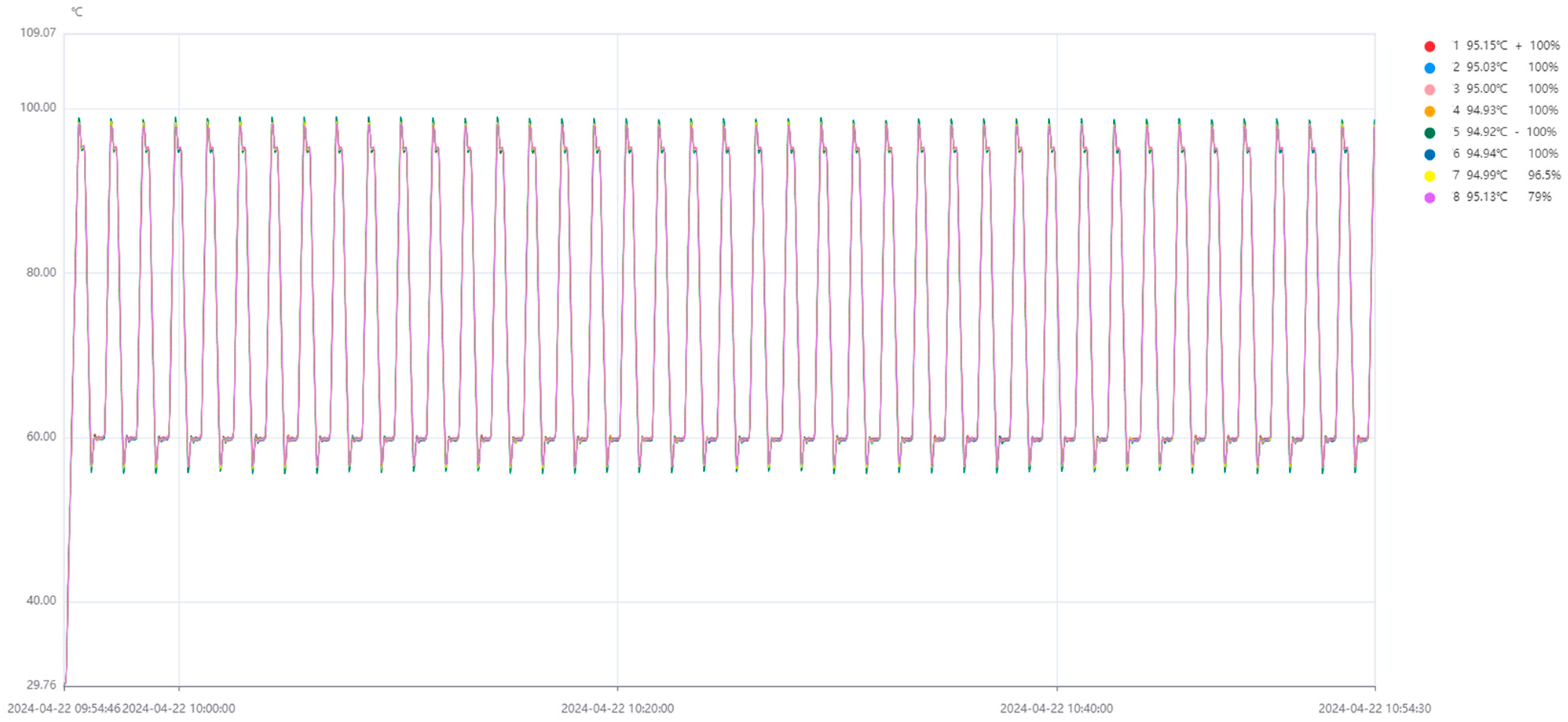
3.1. Temperature Performance Test

Based on the “JJF1821-2020 Temperature Calibration Specification for Polymerase Chain Reaction Analyzers” [31] temperature performance test was conducted using the measurement standards listed in

Table 1. Measurement standards and other equipment for temperature performance test.

Device Name	Model	Manufacturing Number	Manufacturer	Range	Performance
Platinum resistance Thermometer	WZPB-2	11427	DAFANG (Kunming, China)	0–419.5 °C	second class
Digital multimeter	2001	4055379	KEITHLEY (Washington, DC, USA)	100 Ω–100 MΩ	0.0032 + 0.0004 (90 days)
Thermostatic water bath	CJTH-95A	5713	WEILI (Huzhou, China)	+15~95 °C	fluctuation ± 0.01 °C/30 min uniformity < 0.01 °C
Thermostatic oil bath	CJTH-300A	5208	WEILI (Huzhou, China)	90–300 °C	fluctuation ± 0.01 °C/30 min uniformity < 0.01 °C
Isothermal block	CaliTemp-10	86025001	Thermo-leader (Beijing, China)	−40–300 °C	Uniformity: ≤0.03 °C; Fluctuation: ≤0.02 °C/10 min

. The activated calibration device was placed into a fully immersed isothermal block, as depicted in Figure 7a. The eight probes were seamlessly inserted downward into the porous test holes of the isothermal block, ensuring a tight fit between the probes and the isothermal block, and seal the fully immersed isothermal block of the calibration device, as shown in Figure 7b. The sealed, fully immersed isothermal block was sequentially placed into a thermostatic water bath and a thermostatic oil bath, with the immersion depth of the isothermal block not less than 180 mm. The temperature points of the thermostatic bath were set to 0 °C and 120 °C, and the calibration system’s ability to collect corresponding temperatures and meet the temperature measurement range requirements was observed. When the temperature calibration points were 30 °C, 50 °C, 60 °C, 70 °C, and 90 °C, the thermostatic water bath was used. When the temperature calibration point was 95 °C, the thermostatic oil bath was used. After stabilizing for more than half an hour at each calibration temperature point, the calibration device was removed from the bath, and the temperature values of the eight probes measured at the set temperature points were read from the software, and the temperature indication errors were calculated. The temperature performance test results are shown in

Table 2. Temperature performance test results.

No.	Temperature Error/°C						Measurement Uncertainty U, k = 2
	30	50	60	70	90	95
1	+0.02	+0.01	+0.01	+0.01	+0.01	+0.01	0.04
2	+0.01	+0.01	+0.03	+0.01	+0.02	+0.01	0.04
3	+0.01	+0.03	+0.01	+0.02	+0.02	+0.02	0.04
4	+0.02	+0.02	+0.01	+0.01	+0.01	+0.02	0.04
5	+0.01	+0.02	+0.01	+0.01	+0.02	+0.02	0.04
6	+0.02	+0.01	+0.01	+0.01	+0.02	+0.01	0.04
7	+0.02	+0.01	+0.01	+0.01	+0.02	+0.01	0.04
8	+0.01	+0.02	+0.02	+0.03	+0.02	+0.02	0.04

. The maximum error was +0.03 °C, which meets the requirements of calibration specifications.

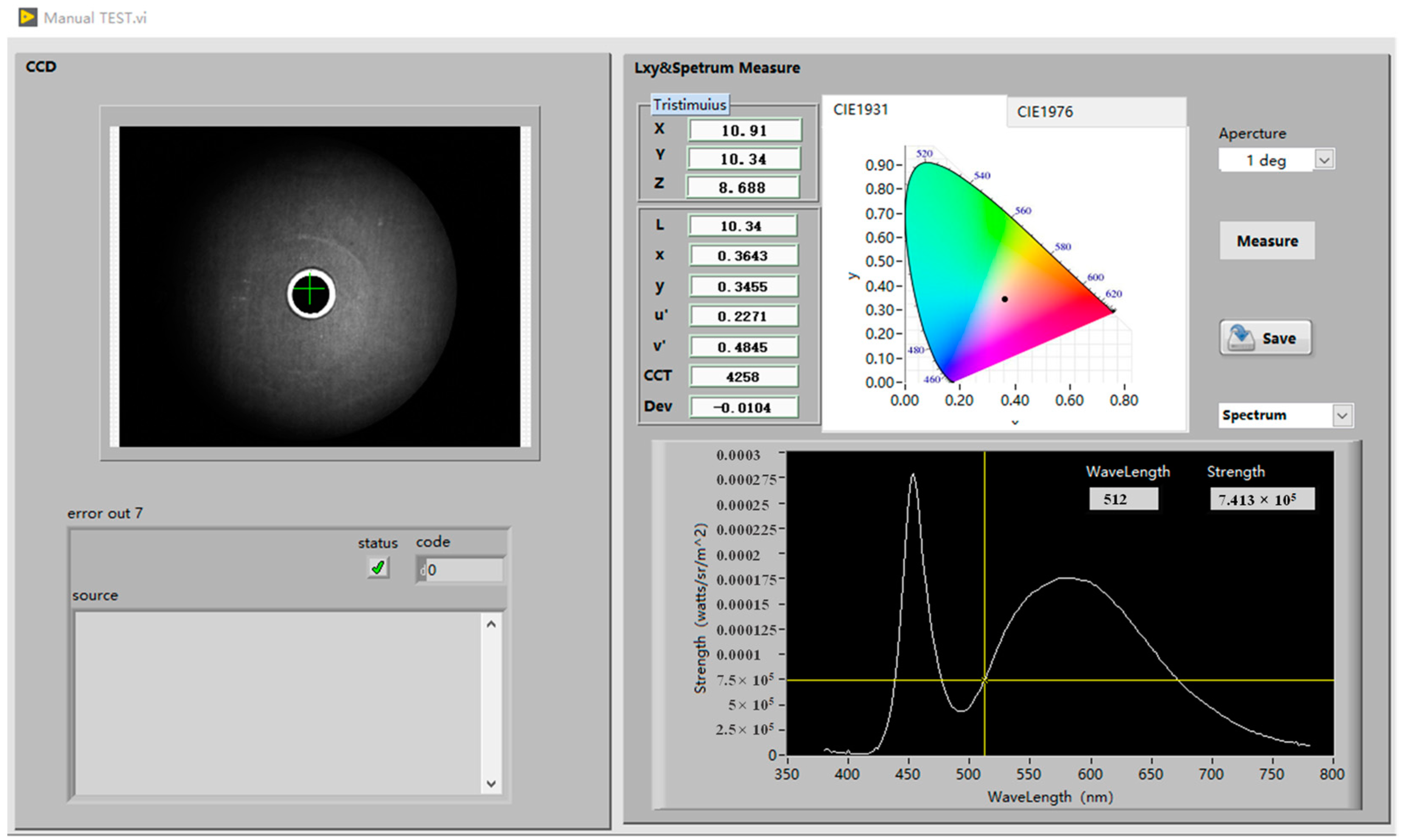
3.2. Optical Performance Test

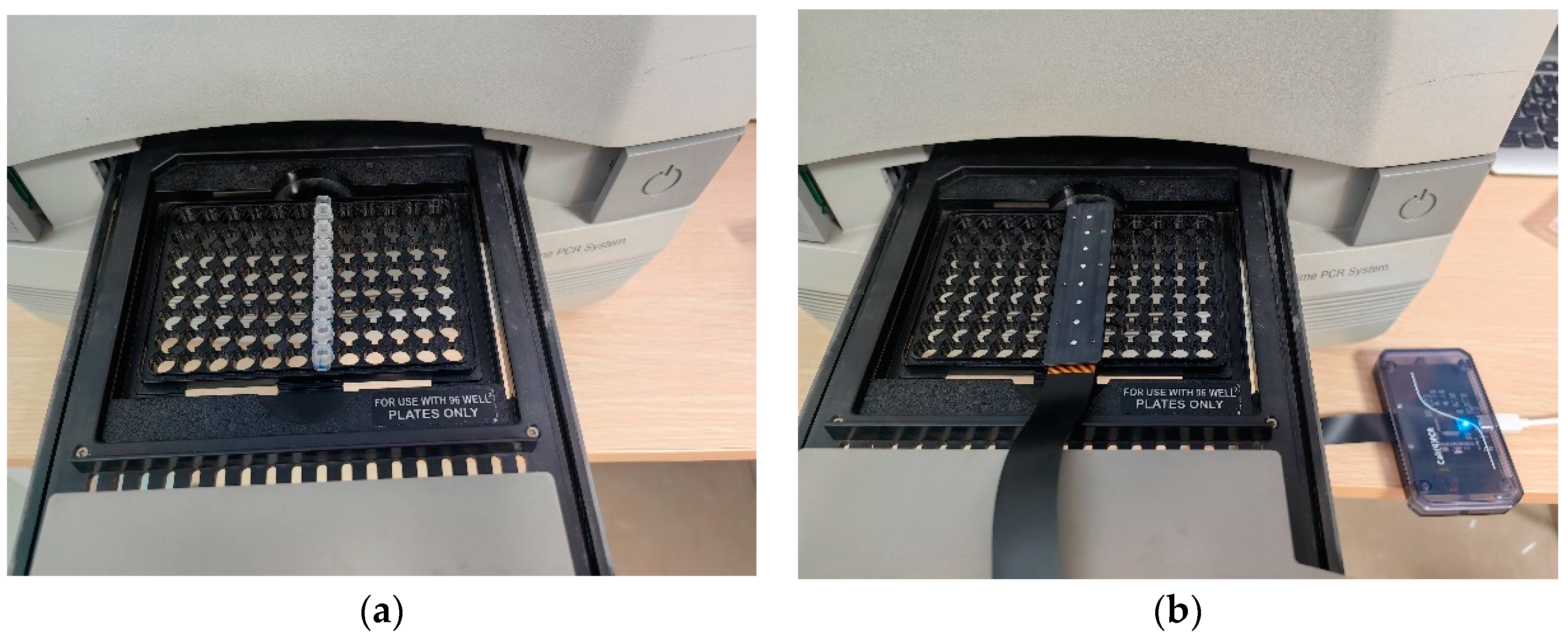
The optical performance testing utilizes a fully automated optical calibration device consisting of a darkroom, spectrometer, a three-axis drive system, and a positioning module. The spectrometer (PR-670) has a luminance measurement range of 0.1 to 1000 cd/cm² and a wavelength measurement range of 360 to 780 nm. It is traceable to national standards and meets relevant specifications. The testing site is shown in Figure 8. We first adjust the spectrometer and guide rail to be level, then adjust the three-axis structure so that the lens of the spectrometer is aligned with the light emitting point of the probe being tested on the same vertical axis. Next, we adjust the distance from the spectrometer lens to the light emitting point to ensure that the center of the spectrum spot coincides with the transmissive point of emitted light under test. We individually adjust the relative brightness of each probe to 10%, 20%, 50%, 60%, 80%, and 100%. We use the spectrometer to test the brightness values of each probe under these six relative luminance conditions, as shown in Figure 9. Linear regression was performed between the relative emission percentages and the measured luminance values, and the linear regression coefficient (r) was calculated as the linear result of the emission light source, as presented in

Table 3. Optical linearity test results of the calibration device.

No.	Measured Luminance Values/cd/m2						r	Measurement Uncertainty ${\mathit{U}}_{\mathbf{r}\mathbf{e}\mathbf{l}}$, k = 2
	100%	80%	60%	50%	20%	10%
1	9.560	7.580	5.658	4.707	1.937	1.0030	0.9999	5.3%
2	9.568	7.572	5.607	4.649	1.900	0.9518	0.9998	5.3%
3	9.707	7.733	5.765	4.790	1.944	0.9817	0.99995	5.3%
4	9.587	7.640	5.714	4.765	2.048	0.9668	0.99985	5.3%
5	9.754	7.766	5.792	4.815	1.984	1.0210	0.99995	5.3%
6	9.818	7.821	5.838	4.860	1.975	0.9292	0.99995	5.3%
7	9.750	7.755	5.772	4.813	1.979	1.0080	0.9999	5.3%
8	9.749	7.752	5.793	4.814	2.019	0.9979	0.9999	5.3%

. The factory linear requirement for qPCR instruments is generally r > 0.997. Typically, the maximum allowable error of measurement standards should not exceed 1/3 of the maximum allowable error of the measured object. The linearity of the calibration device should meet a requirement r ≥ 0.999, and it has been confirmed that this developed calibration device meets this criterion.

4. On-Machine Test

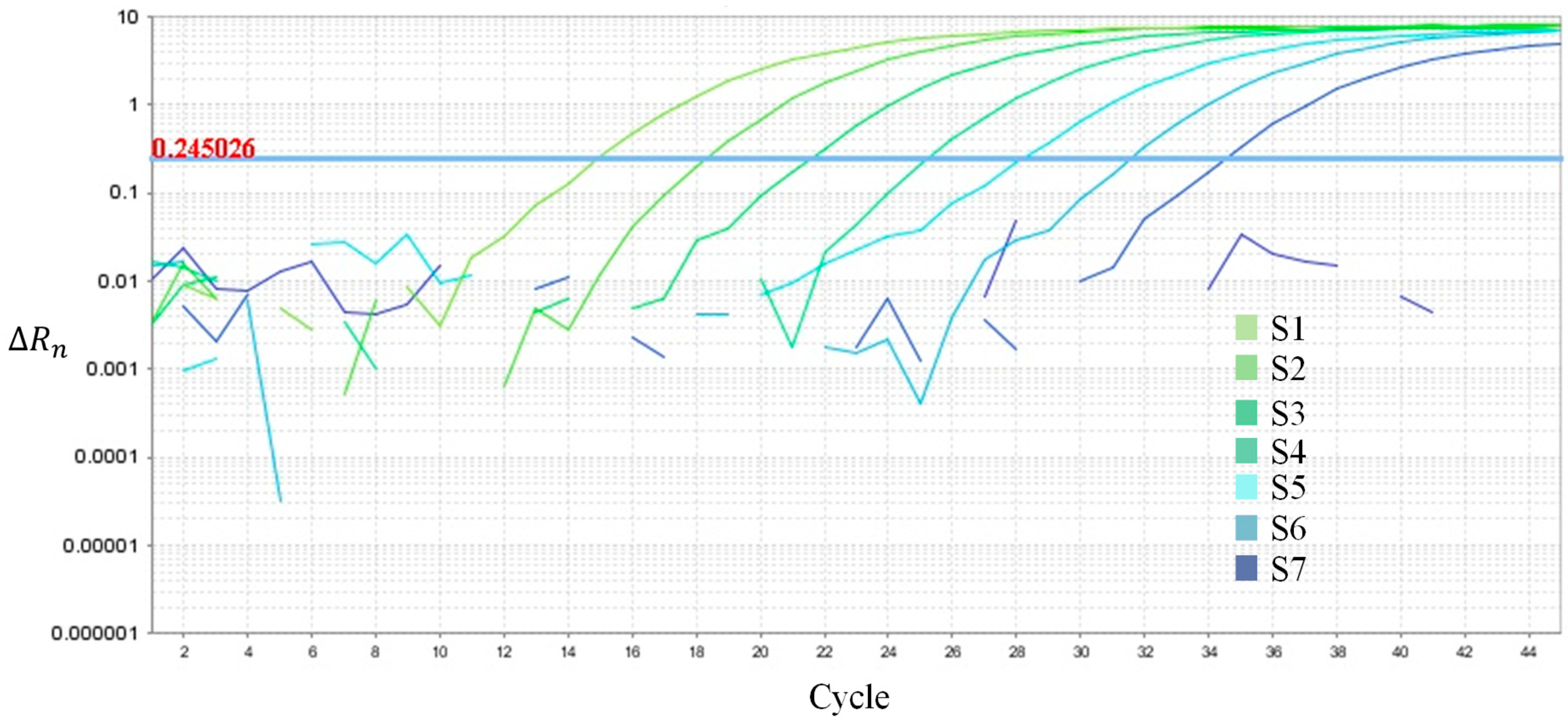
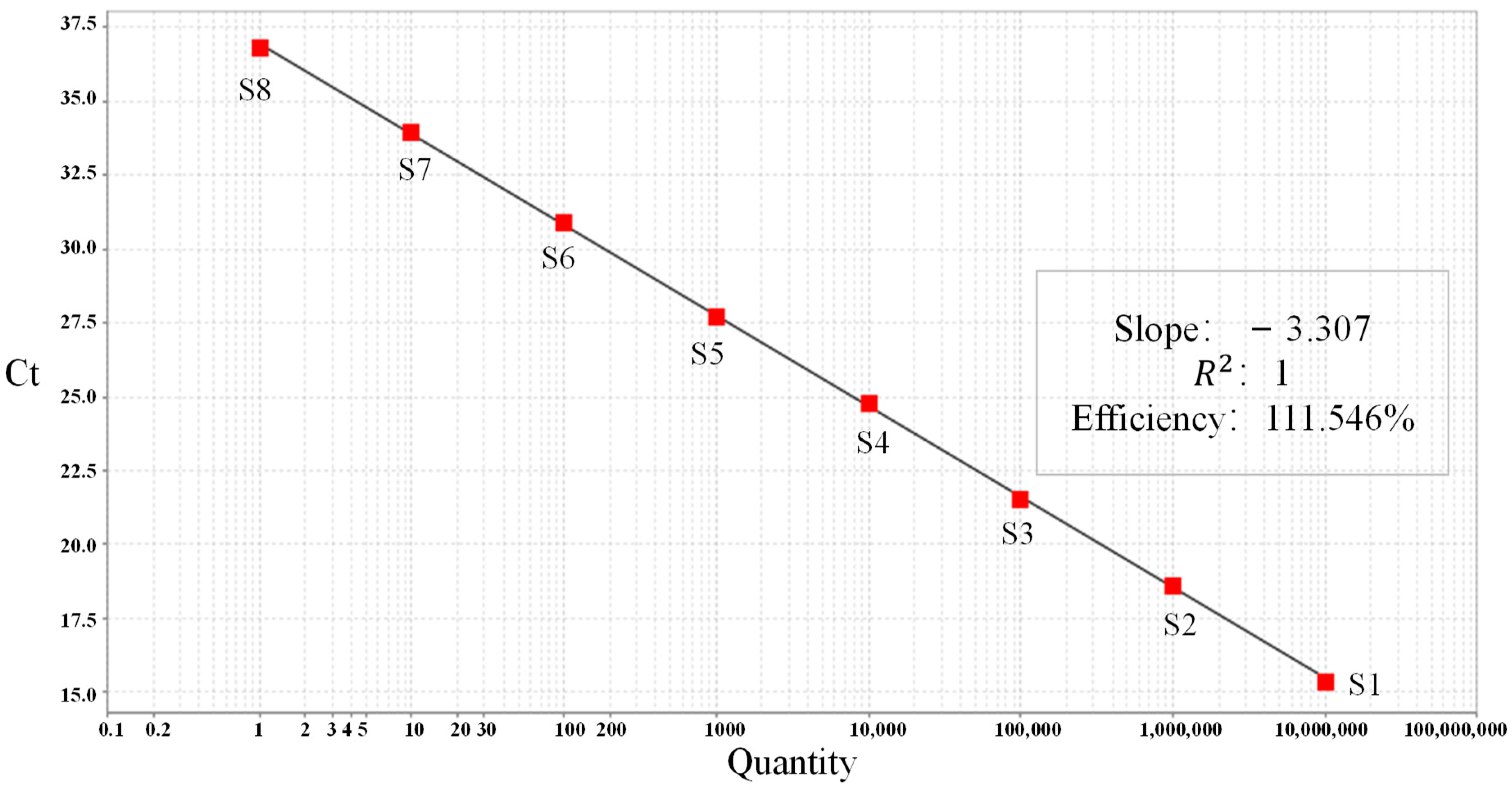
4.1. Standard Curve Simulation

First, a series of diluted standard substances were used to calibrate the sample linearity of the ABI 7500 qPCR instrument, in order to obtain a basic standard curve for simulation and comparative analysis. The standard substance used was the EGFR-1 (18-, 19-, 20-, 21-) gene mutation standard substance, which includes seven different dilution concentrations, as detailed in

Table 4. Reference material details.

Name	Sample Type	Concentration
S1	Standard	1.04 × 107 copies/uL
S2	Standard	1.06 × 106 copies/uL
S3	Standard	1.06 × 105 copies/uL
S4	Standard	1.07 × 104 copies/uL
S5	Standard	1.12 × 103 copies/uL
S6	Standard	1.10 × 102 copies/uL
S7	Standard	1.11 × 101 copies/uL
NTC	Negative control	0

. The standard substance was placed into the 7500 qPCR instrument as depicted in Figure 10a. We set the fluorescence reporter to FAM and the thermal-cycling run method as follows: 50 °C for 2 min once, 95 °C for 10 min once, 95 °C for 30 s, 60 °C for 1 min $\times$ 40 cycles, acquisition is performed in the 60 °C for 1 min step.

The amplification results of the standard substances are shown in Figure 11, and the results are presented in

Table 5. Amplification results of standard substances.

Name	Sample Type	Concentration	Logarithm of Concentration	Measured Ct Value
S1	Standard	1.04 × 107 copies/uL	7	14.934
S2	Standard	1.06 × 106 copies/uL	6	18.284
S3	Standard	1.06 × 105 copies/uL	5	21.440
S4	Standard	1.07 × 104 copies/uL	4	25.243
S5	Standard	1.12 × 103 copies/uL	3	28.333
S6	Standard	1.10 × 102 copies/uL	2	31.497
S7	Standard	1.11 × 101 copies/uL	1	34.488
NTC	Negative control	0	/	undetermined

. A standard curve for standard substances is plotted with the logarithm of the concentrations of the standard substances as the x-axis and the Ct values corresponding to each standard substance as the y-axis, as shown in Figure 12, which was automatically generated by the 7500 qPCR instrument. The regression coefficient representing sample linearity was calculated according to Equation (3). The linear correlation obtained was r = −0.9975 (R² = 0.995). Sample linearity characterizes how closely the regression line of a standard curve fits with Ct values of standards, indicating a high degree of fit between them; when r = 1, it indicates a perfect fit between the regression line and the data points [13].

$$r=\frac{{\sum }_{i=1}^n(C{t}_i-\overline{Ct})(\mathit{ln}{c}_i-\overline{\mathit{ln}c})}{{\sum }_{i=1}^n(C{t}_i-\overline{Ct}{)}^2{\sum }_{i=1}^n(\mathit{ln}{c}_i-\overline{\mathit{ln}c}{)}^2}$$

(3)

where the $r$ represents the linear correlation coefficient; $C{t}_i$ denotes the i-th measured Ct value of serially diluted standard substances; $\overline{Ct}$ is the mean measured Ct value of serially diluted standard substances; $\mathit{ln}{c}_i$ stands for the logarithm of concentration values for the i-th dilution of standard substances; and $\overline{\mathit{ln}c}$ represents the average logarithm of concentration values for serially diluted standard substances.

Since the calibration device relies on the variation in fluorescence intensity at the end of each cycle to simulate the fluorescence changes, Ct values can only be simulated as integers. Based on the distribution of Ct values of the standard substances, simulated Ct values and initial sample concentrations can be estimated. The calibration device has eight probes, which can simulate standard samples with eight different initial concentrations. Taking S1 as an example, the simulated logarithm of concentration value is 7 and the Ct value is 15; for S8, the simulated logarithm of concentration value is 0 and the Ct value is 36. The linear equation for drawing a standard curve with r = 1 would be: $y=-3x+36$. The simulated logarithm of concentration values and Ct values for each probe can be calculated accordingly. The 7500 qPCR instrument under test should be set to the same reporter and run method as the experiment using standard substances. The calibration device was placed in the 7th column of the qPCR, as shown in Figure 10b, and the simulation details were set on the software as shown in

Table 6. Details of the calibration device’s simulated standard curve settings for each probe.

No.	Well’s Position	Simulated Ct Value	Simulated Sample Concentrations	Simulated Sample Logarithm	Simulated Sample Type
1	A7	15	1.0 × 107 copies/uL	7	S1
2	B7	18	1.0 × 106 copies/uL	6	S2
3	C7	21	1.0 × 105 copies/uL	5	S3
4	D7	24	1.0 × 104 copies/uL	4	S4
5	E7	27	1.0 × 103 copies/uL	3	S5
6	F7	30	1.0 × 102 copies/uL	2	S6
7	G7	33	1.0 × 101 copies/uL	1	S7
8	H7	36	1.0 × 100 copies/uL	0	S8

. The simulated standard curves listed in the table can be directly used for reproducibility on other qPCR instruments or a new set of standard curves can be simulated based on requirements.

At this point, the theoretically expected linearity of the standard curve plotted by the calibration device is r = 1. If the actual linearity of the standard curve generated by the qPCR instrument differs from 1, it can be inferred that this difference is caused by issues within the qPCR instrument itself. This difference may arise due to inaccuracies in the optical system, edge effects, or other reasons, and it can be used to analyze the performance issues of the instrument itself.

During the calibration process, the real-time temperature curve collected by the probes and the corresponding fluorescence percentage change based on temperature variation are shown in Figure 13. After calibration, the amplification curves are depicted in Figure 14, while the simulated standard curve generated by the qPCR is presented in Figure 15. The measured actual Ct values are listed in

Table 7. Experimentally measured Ct values of calibration device.

Probe Position	Pre-Set Simulated Ct Value	Experimentally Measured Ct Value
A7	15	15.369
B7	18	18.592
C7	21	21.509
D7	24	24.795
E7	27	27.676
F7	30	30.882
G7	33	33.973
H7	36	36.831

, and based on Equation (3), a linear correlation of R² = 1 is calculated. Based on the calibration results, it is evident that the actual linearity matches the simulated linearity, indicating good performance of the optical detection module of this 7500 qPCR instrument. Any deviation from one, when measuring with standard substances, may be attributed to errors during the gradient dilution process of the standard substances or degradation of DNAs within the standard substances.

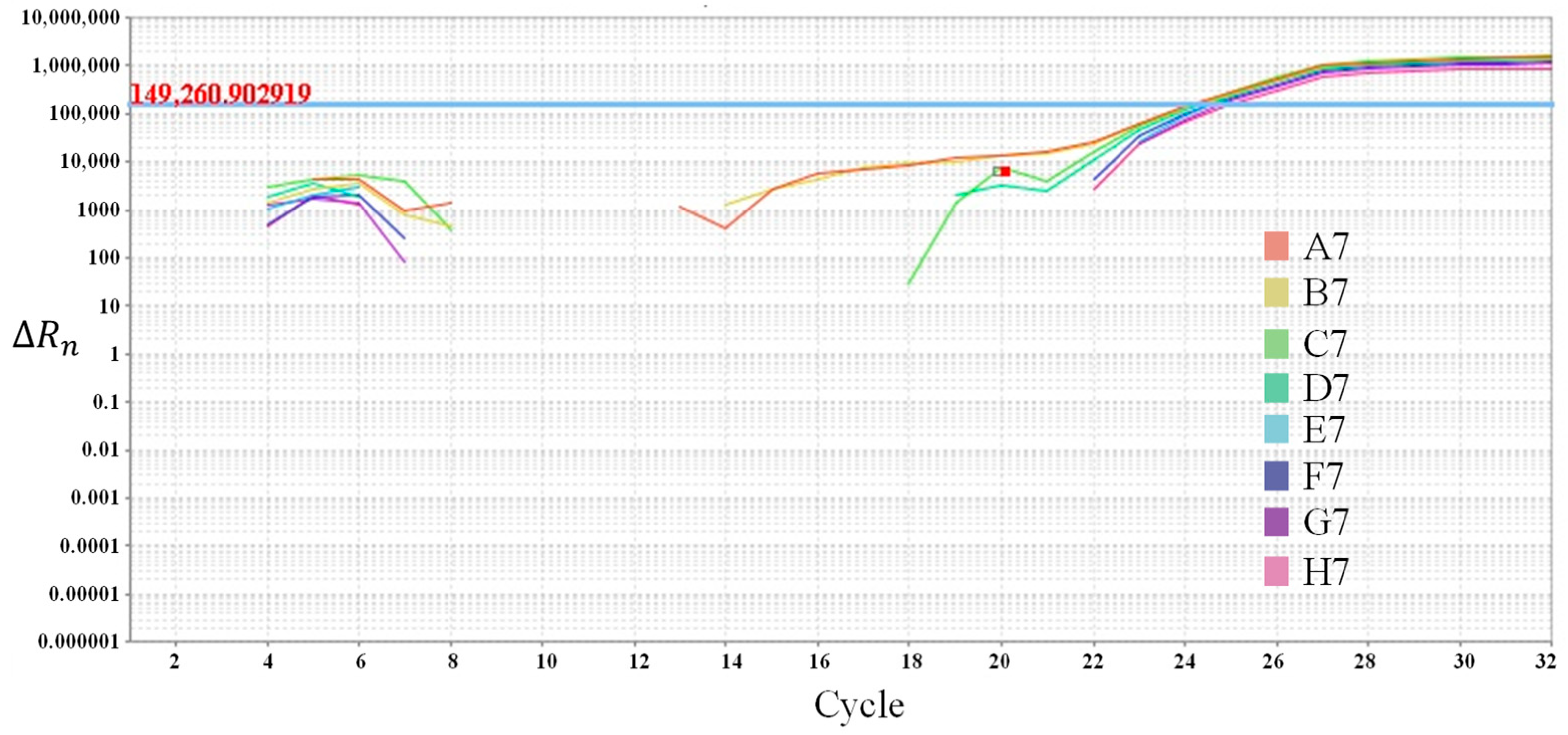
4.2. Uniformity Test

The uniformity test is used to verify the consistency of detection results obtained from different well positions when amplifying samples with the same initial concentration using a qPCR instrument. In theory, the measured Ct values should be identical; however, in practice, they may be influenced by differences in the amount of excitation light received by each reaction well. Some qPCR instruments utilize halogen lamps as their excitation light source, which may experience degradation over time during usage. This degradation could potentially exacerbate the edge effects of the instrument, leading to differences in the amount of excitation light received by reaction wells at different positions. Without re-calibration of the region of interest (ROI), this may impact experimental results.

The calibration device can also be used for uniformity calibration. When testing the uniformity of qPCR instruments using the developed calibration device, the eight probes of the calibration device were set to simulate identical Ct value, all set to 24. The calibration device was then placed in the seventh column and run method settings was set to the same as in Section 4.1.

After running the qPCR process, the amplification curves obtained are shown in Figure 16. The uniformity of Ct values ($\Delta C_{tu}$) can be calculated according to Equation (4), and the precision of Ct values ($RS{D}_{C_t}$) can be calculated according to Equation (5). The results of the uniformity test are presented in

Table 8. The calibration device simulates measured results with identical Ct values.

Probe Position	A7	B7	C7	D7	E7	F7	G7	H7
Measured Ct value	24.18	24.33	24.22	24.45	24.57	24.67	24.78	24.82
Average value	24.50
Uniformity of Ct	0.64
Precision of Ct	1.01%

. The results indicate that when the calibration device simulates identical Ct values, the measured results from the probe within individual reaction wells are not entirely consistent. This discrepancy is caused by inherent differences in the instrument. When analyzing Ct value results for nucleic acid detection in practical use, it is essential to consider the differences introduced by the non-uniformity between reaction wells.

$$\Delta C_{tu}=C_{t\mathrm{qmax}}-C_{t\mathrm{qmin}}$$

(4)

$$RS{D}_{C_t}=\frac{1}{\frac{{\sum }_{i=1}^n{C}_{tqi}}{n}}\times \sqrt{\frac{{\sum }_{i=1}^n(C_{tqi}-\frac{{\sum }_{i=1}^n{C}_{tqi}}{n}{)}^2}{n-1}}\times 100\%$$

(5)

where the $C_{tqi}$ represents the experimentally measured Ct value of the number $i$ probe position; $C_{t\mathrm{qmax}}$ represents the maximum value among the experimentally measured Ct values of all probe positions; $C_{t\mathrm{qmin}}$ represents the minimum value among the experimentally measured Ct values of all probe positions; and $n$ represents the number of probes, n = 8.

In this test, although the calibration results obtained from the standard curve simulation demonstrated a linear correlation of one, a uniformity test on eight wells at the same position revealed discernible differences between the wells. The measured Ct values exhibited variations and deviated from the preset values. It is evident that in standard curve calibration, due to the normalization of linearity calculations, such differences are easily obscured in the final results. Therefore, it is recommended that a comprehensive approach or multiple methods be employed for calibrating and analyzing qPCR instruments.

5. Discussion

The detection of Ct values by qPCR instruments can be influenced by various factors. Additionally, when calibrating the optical parameters of qPCR instruments using biochemical methods, errors resulting from standard substance freeze–thaw cycles, DNA degradation, and serial dilution gradient processes may lead to significant uncertainty in the final linear measurement results. This paper presents the design and development of a calibration device utilizing traceable standard light sources combined with temperature probes. This device enables the simulation of standard curves solely through physical quantity control, facilitating the calibration of both temperature and optical performance of qPCR instruments. By employing this device to simulate standard Ct values and the standard curve, it becomes possible to better mitigate differences in Ct value detection results introduced by other influencing factors. Specifically, the assessment focuses solely on differences in Ct values resulting from temperature non-uniformity and optical detection design flaws in the qPCR instrument.

This paper presents a calibration device based on physical simulation method that incorporates dual temperature and optical calibration functions. This device is capable of real-time acquisition of temperature data from the measured qPCR instruments and can simulate optical amplification. It can be used to simulate uniformity calibration with standard materials of the same concentration and linear calibration with gradient-diluted standard materials for standard curve generation. The potential of this device lies in its ability to address both temperature and optical calibrations, which are typically conducted separately or only focusing on temperature in conventional qPCR instruments performance calibrations [32,33,34,35]. The effects caused by temperature uniformity and fluorescence system noise are often analyzed independently, leading to challenges in verifying differences in temperature uniformity through repeated sample amplification experiments on a 96-well plate [36]. Optical calibration usually relies on biochemical methods for generating standard curves using one or more standard substances [37,38], or comparing positive and negative amplification results from qPCR experiments performed under identical conditions using two or more PCR instruments [39,40]. However, due to variations in qPCR assays performed in different laboratories as well as the diverse nature of standard substances used, direct comparison of quantitative data between different labs becomes challenging [41]. Furthermore, biological method-based calibrations yield composite results that make it difficult to discern subtle differences arising from hardware manufacturing variances within the optical system or discrepancies introduced by biological samples preparation procedures and human error affecting amplification outcomes. Regular comprehensive evaluations of qPCR instruments performance are essential for meeting quality control requirements while ensuring accurate and reliable amplification results. In contrast to biological methods, our proposed physical method offers greater stability and reliability in terms of control.

When employing biological methods for preparing standard curves during calibration processes, these curves are influenced not only by inherent instrument performance but also errors stemming from sample preparation procedures [32], properties associated with dilution buffers [42], precision issues related to pipetting accuracy [43], fluctuations within fluorescence baselines causing measurement errors, DNA extraction efficiency [44,45], systematic drifts observed during standard curve measurements [12], as well as environmental impacts related to storage and transportation [46]. Our proposed physical device effectively mitigates these influences. While a result with a standard curve r ≥ 0.980 is generally considered satisfactory when utilizing biological methods for calibrating purposes, our physical method directly simulates an ideal r = 1-standard curve where any measured deviation is solely linked to qPCR instrument performance.

Moreover, our calibration device encompasses features enabling simultaneous adjustment analyses involving both thermal parameters alongside composite optical parameters compared against single parameter adjustments, such as those focused solely on addressing heating/cooling rate within qPCR instruments [14,47]. Based on the simulation principles provided in this article, it is evident that the application of this device also includes the calibration of multiple-channel optical parameters and physical methods for analyzing melting curves. The resulting calibration results can provide improved assessment and calibration guidance for the use of qPCR instruments. The system can customize simulated Ct values and standard curves based on the characteristics of the standard materials or samples used by the user, offering greater flexibility compared to selecting fixed standard materials and providing more targeted calibration results.

Furthermore, the increasing use of multiplex qPCR instruments for detection has led to a need for multiple fluorescence channels to be utilized simultaneously in order to detect multiple targets and improve detection efficiency. However, this also necessitates the calibration of all fluorescence channels of qPCR instruments [48], typically requiring costly and complex configurations with standard substances containing multiple fluorescent probes. The device developed in this study utilizes LEDs as the standard light source, enabling full-spectrum optical simulation and calibration of different fluorescence channels of the PCR instrument through selection via the device’s filters. This approach not only reduces costs but also offers good reproducibility while achieving simultaneous calibration of multiple channels, thereby saving time and improving overall calibration efficiency. The device provides robust assurance for the application of PCR instruments in molecular biology research. Through performance testing and comparative on-site experiments, we have demonstrated that this calibration device can serve as an alternative method with superior capabilities compared to traditional biochemical approaches, indicating its significant potential for future applications in research settings.

This study also has a limitation. The threshold cycle and the amplification efficiency are two crucial quantitative parameters [49,50]. Through the fluorescence output control of the calibration device, a simulation of specific Ct values is achieved, and standard curve simulations with a linearity of one are realized. However, according to the amplification efficiency calculation, Equation (6) [13,20] is as follows:

$$E={10}^{-\left(\raisebox{1ex}{$1$}\!\left/ \!\raisebox{-1ex}{$\mathrm{slope}$}\right.\right)}-1$$

(6)

The theoretically simulated amplification efficiency of the standard curve is 115%, while the actual amplification efficiency is 111.546%. A slope close to −3.32 indicates optimal, 100% PCR amplification efficiency [12]. When amplifying real biological nucleic acid samples, the ideal PCR reaction amplification efficiency typically ranges from 90% to 110% [51]. However, due to limitations in control with our calibration device, only integer values of Ct can be simulated. As a result, the amplification efficiency cannot be controlled within the ideal range. Further refinement of the control parameters for optical changes is needed to achieve a more precise simulation of the standard curve. We can enhance the control conditions for optical changes based on the existing framework. The next step involves modifying the current method of controlling optical changes, which relies solely on the number of temperature cycles, to a method that incorporates both the number of temperature cycles and the hold time after reaching that cycle as control conditions for optical changes. For instance, in the current calibration procedure, a temperature gradient of 60 °C is held for 60 s during fluorescence collection. This hold time can be subdivided to enable the calibration device to simulate Ct values with non-integer decimal numbers at the 24th cycle, and after half of the hold time has elapsed, if the temperature change of the optical probe exceeds a certain threshold, it can simulate an amplification curve with a Ct value of 24.5, thus achieving a more comprehensive and functionally diverse simulation. Naturally, this necessitates further refinement of algorithms and optical drive control, and we will conduct additional research to optimize the calibration device.

6. Conclusions

This paper presents a calibration device based on a physical simulation method that incorporates dual temperature and optical calibration functions. This device is capable of real-time acquisition of temperature data from the measured qPCR instruments and could simulate optical amplification. It could be used to simulate uniformity calibration with standard materials of the same concentration. By controlling the output fluorescence through monitoring temperature collection, different probes could simulate different Ct values corresponding to samples with varying initial concentrations, thus simulating a standard curve using a physical device and calibrating qPCR instruments. The different probes of the device were independently controlled, and a single malfunction did not affect the operation of others. The probes were assembled and fixed in a nested manner, allowing for various arrangement options. The 8-probe unit served as the basic unit, which can be used individually or in combination with multiple units to expand its application for calibration of 8-well, 16-well, 48-well, and 96-well qPCR instruments. Furthermore, this device could perform the functions of other physical calibration devices. It could comprehensively, controllably, and traceably replace standard substances for qPCR instrument calibration, ensuring the accuracy of equipment usage.

References

1. Bag, S.; Ghosh, S.; Lalwani, R.; Vishnoi, P.; Gupta, S.; Dubey, D. Real-Time Polymerase Chain Reaction-Based Detection and Quantification of Hepatitis B Virus DNA. J. Vis. Exp. 2023, 15, e66249. [Google Scholar] [CrossRef] [PubMed]
2. Tavares, E.R.; de Lima, T.F.; Bartolomeu-Gonçalves, G.; de Castro, I.M.; de Lima, D.G.; Borges, P.H.G.; Nakazato, G.; Kobayashi, R.K.T.; Venancio, E.J.; Tarley, C.R.T.; et al. Development of a melting-curve-based multiplex real-time PCR assay for the simultaneous detection of viruses causing respiratory infection. Microorganisms 2023, 11, 2692. [Google Scholar] [CrossRef] [PubMed]
3. Zhang, Y.; Zhang, W.; Du, H.; Qu, X.; Chen, Y.; Wang, J.; Wu, R. A comparative analysis of cycle threshold (Ct) values from Cobas4800 and AmpFire HPV assay for triage of women with positive hrHPV results. BMC Infect. Dis. 2023, 23, 783. [Google Scholar] [CrossRef] [PubMed]
4. Shibanuma, T.; Nunomura, Y.; Oba, M.; Kawahara, F.; Mizutani, T.; Takemae, H. Development of a one-run real-time PCR detection system for pathogens associated with poultry infectious diseases. J. Veter. Med. Sci. 2023, 85, 407–411. [Google Scholar] [CrossRef] [PubMed]
5. McDonald, C.; Taylor, D.; Linacre, A. PCR in Forensic Science: A Critical Review. Genes 2024, 15, 438. [Google Scholar] [CrossRef] [PubMed]
6. Jing, Q.; Liu, S.; Song, Y.; Tao, X. TaqMan real-time quantitative PCR for the detection of beef tallow to assess the authenticity of edible oils. Food Control 2024, 156, 110139. [Google Scholar] [CrossRef]
7. Doi, M.; Nakagawa, T.; Asano, M. A practical workflow for forensic species identification using direct sequencing of real-time PCR products. Mol. Biol. Rep. 2023, 51, 17. [Google Scholar] [CrossRef] [PubMed]
8. Li, G.-W.; Luo, Y.-Q.; Fan, Y.-Y.; Xian, L.-Y.; Song, Y.; Chen, X.-D.; Luo, W.-H.; Sun, D.-M.; Wei, M. Species identification of Bungarus multicinctus, Bungarus fasciatus, and Lycodon rufozonatus in Chinese medicinal crude drugs and extracts using capillary electrophoresis-based multiplex PCR. Chin. J. Anal. Chem. 2023, 51, 100272. [Google Scholar] [CrossRef]
9. Acquier, M.; Zabala, A.; de Précigout, V.; Delmas, Y.; Dubois, V.; de la Faille, R.; Rubin, S.; Combe, C.; M‘Zali, F.; Kaminski, H. Performance of real-time PCR in suspected haemodialysis catheter-related bloodstream infection: A proof-of-concept study. Clin. Kidney J. 2023, 16, 494–500. [Google Scholar] [CrossRef]
10. Dinç, H.; Yiğin, A.; Koyuncu, I.; Aslan, M. Investigation of the anticancer and apoptotic effect of Micromeria congesta under in vitro conditions and detection of related genes by real-time PCR. In Veterinary Research Forum; Faculty of Veterinary Medicine, Urmia University: Urmia, Iran, 2022; Volume 13. [Google Scholar]
11. Artika, I.M.; Dewi, Y.P.; Nainggolan, I.M.; Siregar, J.E.; Antonjaya, U. Real-time polymerase chain reaction: Current techniques, applications, and role in COVID-19 diagnosis. Genes 2022, 13, 2387. [Google Scholar] [CrossRef]
12. Nagelkerke, E.; Hetebrij, W.A.; Koelewijn, J.M.; Kooij, J.; van der Drift, A.M.R.; van der Beek, R.F.; de Jonge, E.F.; Lodder, W.J. PCR standard curve quantification in an extensive wastewater surveillance program: Results from the Dutch SARS-CoV-2 wastewater surveillance. Front. Public Health 2023, 11, 1141494. [Google Scholar] [CrossRef]
13. Sahoo, S.; Mandal, S.; Das, P.; Bhattacharya, S.; Chandy, M. An analysis of the standard curve parameters of cytomegalovirus, BK virus and hepatitis B virus quantitative polymerase chain reaction from a clinical virology laboratory in eastern India. Indian J. Med. Microbiol. 2022, 40, 81–85. [Google Scholar] [CrossRef]
14. Ling, W.; Zhou, W.; Cui, J.; Shen, Z.; Wei, Q.; Chu, X. Experimental study on the heating/cooling and temperature uniformity performance of the microchannel temperature control device for nucleic acid PCR amplification reaction of COVID-19. Appl. Therm. Eng. 2023, 226, 120342. [Google Scholar] [CrossRef]
15. Liu, H.; Fang, Y.; Su, X.; Wang, Y.; Ji, M.; Xing, H.; Gao, Y.; Zhang, Y.; He, N. Temperature control algorithm for polymerase chain reaction (PCR) instrumentation based upon improved hybrid fuzzy proportional integral derivative (PID) control. Instrum. Sci. Technol. 2023, 51, 109–131. [Google Scholar] [CrossRef]
16. Xi, B.; Huang, S.; An, Y.; Gong, X.; Yang, J.; Zeng, J.; Ge, S.; Zhang, D. Sophisticated and precise: Design and implementation of a real-time optical detection system for ultra-fast PCR. RSC Adv. 2023, 13, 19770–19781. [Google Scholar] [CrossRef] [PubMed]
17. Yang, D.; Hansel, D.E.; Curlin, M.E.; Townes, J.M.; Messer, W.B.; Fan, G.; Qin, X. Bimodal distribution pattern associated with the PCR cycle threshold (Ct) and implications in COVID-19 infections. Sci. Rep. 2022, 12, 14544. [Google Scholar] [CrossRef]
18. Markewitz, R.; Dargvainiene, J.; Junker, R.; Wandinger, K.P. Cycle threshold of SARS-CoV-2 RT-PCR as a driver of retesting. Sci. Rep. 2024, 14, 2423. [Google Scholar] [CrossRef]
19. Abdulrahman, A.; I Mallah, S.; Alawadhi, A.; Perna, S.; Janahi, E.M.; AlQahtani, M.M. Association between RT-PCR Ct values and COVID-19 new daily cases: A multicenter cross-sectional study. Le Infez. Med. 2021, 29, 416. [Google Scholar]
20. Schmidt, P.J.; Acosta, N.; Chik, A.H.S.; D’aoust, P.M.; Delatolla, R.; Dhiyebi, H.A.; Glier, M.B.; Hubert, C.R.J.; Kopetzky, J.; Mangat, C.S.; et al. Realizing the value in “non-standard” parts of the qPCR standard curve by integrating fundamentals of quantitative microbiology. Front. Microbiol. 2023, 14, 1048661. [Google Scholar] [CrossRef]
21. Sala, E.; Shah, I.S.; Manissero, D.; Juanola-Falgarona, M.; Quirke, A.M.; Rao, S.N. Systematic review on the correlation between SARS-CoV-2 real-time PCR cycle threshold values and epidemiological trends. Infect. Dis. Ther. 2023, 12, 749–775. [Google Scholar] [CrossRef]
22. Jeon, B.R. Variation in PCR efficiencies between quantification standards and clinical specimens using different real-time quantitative PCR interpretation methods. Int. J. Biol. Biomed. Eng. 2020, 14, 39–42. [Google Scholar]
23. Olveira, J.G.; Souto, S.; Bandín, I.; Dopazo, C.P. Development and validation of a SYBR green real time PCR protocol for detection and quantification of nervous necrosis virus (NNV) using different standards. Animals 2021, 11, 1100. [Google Scholar] [CrossRef] [PubMed]
24. Li, C.; Hughes, C.; Ding, R.; Snopkowski, C.; Salinas, T.; Schwartz, J.; Dadhania, D.; Suthanthiran, M. Development of a Bak gene based standard curve for absolute quantification of BK virus in real time quantitative PCR assay and noninvasive diagnosis of BK virus nephropathy in kidney allograft recipients. J. Immunol. Methods 2022, 509, 113341. [Google Scholar] [CrossRef] [PubMed]
25. Bonacorsi, S.; Visseaux, B.; Bouzid, D.; Pareja, J.; Rao, S.N.; Manissero, D.; Hansen, G.; Vila, J. Systematic review on the correlation of quantitative PCR cycle threshold values of gastrointestinal pathogens with patient clinical presentation and outcomes. Front. Med. 2021, 8, 711809. [Google Scholar] [CrossRef] [PubMed]
26. Bouzid, D.; Vila, J.; Hansen, G.; Manissero, D.; Pareja, J.; Rao, S.N.; Visseaux, B. Systematic review on the association between respiratory virus real-time PCR cycle threshold values and clinical presentation or outcomes. J. Antimicrob. Chemother. 2021, 76 (Suppl. 3), iii33–iii49. [Google Scholar] [CrossRef] [PubMed]
27. Du, Z.; Behrens, S.F. Effect of target gene sequence evenness and dominance on real-time PCR quantification of artificial sulfate-reducing microbial communities. PLoS ONE 2024, 19, e0299930. [Google Scholar] [CrossRef] [PubMed]
28. Leta, D.; Gutema, G.; Hagos, G.G.; Diriba, R.; Bulti, G.; Sura, T.; Ayana, D.; Chala, D.; Lenjiso, B.; Bulti, J.; et al. Effect of heat inactivation and bulk lysis on real-time reverse transcription PCR detection of the SARS-COV-2: An experimental study. BMC Res. Notes 2022, 15, 295. [Google Scholar] [CrossRef] [PubMed]
29. Goyal, S.; Singh, P.; Sengupta, S.; Muthukrishnan, A.B.; Jayaraman, G. DNA-Aptamer-Based qPCR Using Light-Up Dyes for the Detection of Nucleic Acids. ACS Omega 2023, 8, 47277–47282. [Google Scholar] [CrossRef]
30. Goyal, S.; Singh, P.; Sengupta, S.; Muthukrishnan, A.B.; Jayaraman, G. Performance evaluation of QuantStudio 1 plus real-time PCR instrument for clinical laboratory analysis: A proof-of-concept study. Pract. Lab. Med. 2023, 36, e00330. [Google Scholar]
31. JJF 1821-2020; Calibration Specification of Temperature Calibration Device for Polymerase China Reaction Analyzers. China Quality and Standards Publishing & Media Co., Ltd.: Beijing, China, 2020. Available online: http://jjg.spc.org.cn/resmea/view/stdonline (accessed on 25 April 2024).
32. Li, X.; Nguyen, L.V.; Hill, K.; Ebendorff-Heidepriem, H.; Schartner, E.P.; Zhao, Y.; Zhou, X.; Zhang, Y.; Warren-Smith, S.C. All-fiber all-optical quantitative polymerase chain reaction (qPCR). Sens. Actuators B Chem. 2020, 323, 128681. [Google Scholar] [CrossRef]
33. Span, M.; Verblakt, M.; Hendrikx, T. Measurement uncertainty in calibration and compliancy testing of PCR and qPCR thermal cyclers. In Proceedings of the 18th International Congress of Metrology, Paris, France, 19–21 September 2017; EDP Sciences: Les Ulis, France, 2017. [Google Scholar]
34. Gaňová, M.; Wang, X.; Yan, Z.; Zhang, H.; Lednický, T.; Korabečná, M.; Neužil, P. Temperature non-uniformity detection on dPCR chips and temperature sensor calibration. RSC Adv. 2022, 12, 2375–2382. [Google Scholar] [CrossRef] [PubMed]
35. Tsai, H.-Y.; Chao, L.-C.; Hsu, C.-N.; Huang, K.-C.; Tsai, Y.-H.; Shieh, D.-B.; Yang, C.-C. Development of Non-contact Composite Temperature Sensing (CTS) for photothermal Real-time quantitative PCR Device. In Proceedings of the 2020 IEEE Sensors Applications Symposium (SAS), Kuala Lumpur, Malaysia, 9–11 March 2020. [Google Scholar]
36. Luque-Perez, E.; Mazzara, M.; Weber, T.P.; Foti, N.; Grazioli, E.; Munaro, B.; Pinski, G.; Bellocchi, G.; Eede, G.V.D.; Savini, C. Testing the robustness of validated methods for quantitative detection of GMOs across qPCR instruments. Food Anal. Methods 2013, 6, 343–360. [Google Scholar] [CrossRef]
37. Willis, J.R.; Sivaganesan, M.; Haugland, R.A.; Kralj, J.; Servetas, S.; Hunter, M.E.; Jackson, S.A.; Shanks, O.C. Performance of NIST SRM® 2917 with 13 recreational water quality monitoring qPCR assays. Water Res. 2022, 212, 118114. [Google Scholar] [CrossRef] [PubMed]
38. Chen, S.; Gong, P.; Zhang, J.; Shan, Y.; Han, X.; Zhang, L. Use of qPCR for the analysis of population heterogeneity and dynamics during Lactobacillus delbrueckii spp. bulgaricus batch culture. Artif. Cells Nanomed. Biotechnol. 2021, 49, 1–10. [Google Scholar] [PubMed]
39. Josefsen, M.H.; Löfström, C.; Hansen, T.; Reynisson, E.; Hoorfar, J. Instrumentation and fluorescent chemistries used in qPCR. In Quantitative Real-Time PCR in Applied Microbiology; Caister Academic Press: Wymondham, UK, 2012; pp. 27–52. [Google Scholar]
40. Sivaganesan, M.; Willis, J.R.; Karim, M.; Babatola, A.; Catoe, D.; Boehm, A.B.; Wilder, M.; Green, H.; Lobos, A.; Harwood, V.J.; et al. Interlaboratory performance and quantitative PCR data acceptance metrics for NIST SRM® 2917. Water Res. 2022, 225, 119162. [Google Scholar] [CrossRef] [PubMed]
41. Beinhauerova, M.; Beinhauerova, M.; McCallum, S.; Sellal, E.; Ricchi, M.; O’Brien, R.; Blanchard, B.; Slana, I.; Babak, V.; Kralik, P. Development of a reference standard for the detection and quantification of Mycobacterium avium subsp. paratuberculosis by quantitative PCR. Sci. Rep. 2021, 11, 11622. [Google Scholar] [CrossRef] [PubMed]
42. Ruijter, J.M.; Barnewall, R.J.; Marsh, I.B.; Szentirmay, A.N.; Quinn, J.C.; van Houdt, R.; Gunst, Q.D.; Hoff, M.J.B.v.D. Efficiency correction is required for accurate quantitative PCR analysis and reporting. Clin. Chem. 2021, 67, 829–842. [Google Scholar] [CrossRef] [PubMed]
43. Grgicak, C.M.; Urban, Z.M.; Cotton, R.W. Investigation of reproducibility and error associated with qPCR methods using Quantifiler® Duo DNA quantification kit. J. Forensic Sci. 2010, 55, 1331–1339. [Google Scholar] [CrossRef] [PubMed]
44. Span, M.; Verblakt, M.; Hendrikx, T. Comparison of temperature dynamics of various thermal cycler calibration methods. In Proceedings of the 19th International Congress of Metrology (CIM2019), Paris, France, 24–26 September 2019; EDP Sciences: Les Ulis, France, 2019; p. 19003. [Google Scholar]
45. Lima, Â.; Sousa, L.G.; Cerca, N. Accurate absolute quantification of bacterial populations in mixed cultures by qPCR. In PCR: Methods and Protocols; Springer: New York, NY, USA, 2023; pp. 105–115. [Google Scholar]
46. Morinha, F.; Magalhães, P.; Blanco, G. Standard guidelines for the publication of telomere qPCR results in evolutionary ecology. Mol. Ecol. Resour. 2020, 20, 635–648. [Google Scholar] [CrossRef]
47. Dawson, P.; Buyukyavuz, A.; Ionita, C.; Northcutt, J. Effects of DNA extraction methods on the real time PCR quantification of Campylobacter jejuni, Campylobacter coli, and Campylobacter lari in chicken feces and ceca contents. Poult. Sci. 2023, 102, 102369. [Google Scholar] [CrossRef]
48. Zhu, H.; Liu, X.; Wang, Y.; Sun, A.; Teplý, T.; Korabečná, M.; Zhang, H.; Neuzil, P. Smallest dual-color qPCR device. Sens. Actuators B Chem. 2023, 394, 134299. [Google Scholar] [CrossRef]
49. Ramezani, A. CtNorm: Real time PCR cycle of threshold (Ct) normalization algorithm. J. Microbiol. Methods 2021, 187, 106267. [Google Scholar] [CrossRef] [PubMed]
50. Just, V.M.; Welzel, F.; Jacobs, H.; Gau, G.; Hauschultz, M.T.; Friedo, M.H.; Foitzik, A.H. Development of a Thermal Cycler for a Low-Cost Real-Time PCR Application. Key Eng. Mater. 2023, 968, 73–79. [Google Scholar] [CrossRef]
51. Chen, Z.; Halford, N.G.; Liu, C. Real-time quantitative PCR: Primer design, reference gene selection, calculations and statistics. Metabolites 2023, 13, 806. [Google Scholar] [CrossRef]
Figure 1. Schematic diagram of calibration device.
Applsci 14 05031 g001
Figure 2. Relative luminous intensity change process of the probe with the number of cycles.
Applsci 14 05031 g002
Figure 3. Calibration device probe control flow chart when the simulated Ct value is 24.
Applsci 14 05031 g003
Figure 4. Overall structure design (a) and diagram (b) of calibration device.
Applsci 14 05031 g004
Figure 5. Implementation diagram of the calibration device. (a) Physical representation of the calibration device. (b) The state picture when all eight probes of the calibration device emit the same light.
Applsci 14 05031 g005
Figure 6. Overall experimental design.
Applsci 14 05031 g006
Figure 7. Full immersion isothermal block seal calibration device. (a) Calibration device probe placement state. (b) Calibration device seal status.
Applsci 14 05031 g007
Figure 8. Optical calibration site.
Applsci 14 05031 g008
Figure 9. Measured luminance results when the relative luminance of a probe is 100%.
Applsci 14 05031 g009
Figure 10. On-machine test scene. (a) On-machine test of standard substances. (b) On-machine test of calibration device.
Applsci 14 05031 g010
Figure 11. Measured amplification curves of serially diluted standard substances.
Applsci 14 05031 g011
Figure 12. Measured standard curve of serially diluted standard substances.
Applsci 14 05031 g012
Figure 13. Real-time temperature curve and optical variation.
Applsci 14 05031 g013
Figure 14. Experimentally measured amplification plot of the calibration device.
Applsci 14 05031 g014
Figure 15. Experimentally measured standard curve of the calibration device.
Applsci 14 05031 g015
Figure 16. Experimental amplification plot when simulate identical Ct values.
Applsci 14 05031 g016