Abstract
This study investigating the accuracy of turbulence model simulations of the exhaust manifold using computational fluid dynamics (CFD) carries significant implications. By modeling and analyzing the flow of emissions, we aim to identify areas of high stress and pressure, minimize the pressure drop, and maximize the flow of exhaust gases. This not only enhances engine performance, reduces emissions, and improves the durability of the manifold but also provides a unique opportunity to predict and analyze the flow and performance of the exhaust manifold, both quantitatively and qualitatively. This paper aims to provide a detailed comparison of five turbulence models that are commonly used in CFD to offer valuable insights into their accuracy and reliability in predicting the flow characteristics of exhaust gases. The results show that the k-kl-ω model showed the highest maximum velocity and the most comprehensive temperature range, efficiently capturing the transitional flow effects. The K-ω STD and SST transition models displayed significantly higher turbulent kinetic energy (TKE) values, indicating their enhanced effectiveness in modeling complex turbulent and transitional flows. Conversely, the Reynolds stress and RNG k-epsilon models displayed lower TKE values, suggesting more subdued turbulence predictions. Despite this, all models exhibited similar pressure drop trends, with a noticeable increase near the midpoint of the manifold. These quantitative findings provide valuable insights into the suitability of different turbulence models for optimizing exhaust manifold design.
1. Introduction
The exhaust manifold is a fundamental component within the vehicle’s infrastructure, serving the essential function of expelling harmful gases emanating from the engine (see Soares et al. [1], Cheng et al. [2], and Chaudhari et al. [3]). The primary objective of this critical subsystem revolves around the reduction of noise and the effective control of emissions. In the context of a scientific article, understanding and optimizing the exhaust manifold’s role is imperative for advancing both vehicle performance and environmental considerations.
Turbulence is a complex phenomenon that is a challenge for precise modeling in CFD simulations. A range of turbulence models is available, each with its own limitations and assumptions, underscoring the importance of selecting the most suitable model for our study. Leveraging CFD methods allows for the simulation of flow patterns within the exhaust manifold, facilitating the optimization of its design parameters (see Wang et al. [4] and Cihan et al. [5]). The primary aim of this study is to conduct a transient CFD analysis of an exhaust manifold using five turbulence models. The objective is to compare these models and identify the most accurate one for predicting velocity, temperature, and turbulent kinetic energy within the exhaust manifold.
Many studies have been conducted to compare different turbulence models for different flow situations. Bral et al. [6] discussed using CFD simulations to analyze an exhaust manifold’s flow and emissions characteristics. The objective of the study was to find ways to decrease emissions by enhancing the design of the manifold. This research offers significant insights into the use of CFD simulations to optimize exhaust manifold designs to reduce emissions. The results of this study can be utilized to create more efficient and environmentally friendly automotive engines.
Haoran and Jianhong [7] compared the performance of five turbulence models when modeling the nearshore hydrodynamics of coral reefs using the open-source solver OlaFlow. They found that the k-omega SST turbulence model showed the best agreement with the field measurements, followed by the k-epsilon turbulence model. The standard k-omega model was unsuitable for modeling the coral reefs’ nearshore hydrodynamics, due to its inability to capture complex flow patterns.
Ajayi et al. [8] underscore the critical importance of accurately predicting airflow around turbine rotors to optimize wind farm layout design. The study evaluates numerical turbulence models, including Reynolds-Averaged Navier Stokes (RANS) and two-equation transport models k-ε and k-ω, emphasizing their respective strengths and limitations. The findings indicate that the k-ω model, particularly the combinatorial shear stress transport version, offers a comparative advantage in resolving eddies and addressing the closure problem.
Cen [9] compared two turbulence models, omega RSM and RNG k-ε, to simulate a hydro cyclone used in mineral processing. The Eulerian-Eulerian approach was used to simulate water and solid particle flow. Both models were compared based on velocity field, pressure drop, and separation efficiency. The omega RSM model provided a more accurate prediction of the velocity field near the wall.
Huang et al. [10] compared a developed SST k-ω turbulence model with other turbulence models for predicting turbulent slot jet impingement in heat transfer. CFD simulations were used, showing that the SST k-ω turbulence model provided more accurate predictions of the heat transfer coefficient. The model captured primary features such as the jet impingement zone, the wall jet, and the recirculation zone.
Cabello et al. [11] investigated the heat transfer characteristics of pipes with twisted tapes using CFD simulations and experimental validation. Twisted tapes promote turbulent flow and enhance heat transfer by creating vortices. The study found that a horizontal pipe with a twisted tape insert significantly improved the heat transfer rate in both laminar and turbulent flow regimes. The CFD simulations were in good agreement with the experimental data, validating the accuracy of the model.
Eroglu et al. [12] presented a theoretical analysis that evaluated three distinct computer-aided engineering (CAE) methodologies for simulating fluid flow and thermal distribution in the exhaust manifold of a heavy-duty diesel engine. The fluid flow pulsations in the engine exhaust manifold represented a significant level of complexity. Consequently, experimental measurements of the manifold temperatures were conducted to validate the results obtained from each CAE approach. The predicted metal temperature was subsequently utilized to carry out a thermo-structural durability analysis. It is noteworthy, however, that assessing the exhaust manifold design of the HD diesel engine extends beyond the parameters of the present study.
Moen et al. [13] compared k-epsilon turbulence models for simulating gas release and dispersion using the FLACS CFD code. The study identified the most appropriate k-epsilon model for simulating gaseous release in complex environments. The three models analyzed were the standard, RNG, and realizable k-epsilon models. The realizable k-epsilon model provided the best results, while the standard k-epsilon model was the most computationally efficient. The RNG k-epsilon model predicted the turbulence intensity most accurately.
Allawi et al. [14] analyzed the exhaust manifold of a four-stroke, four-cylinder, spark-ignition engine using three different fuels: gasoline, methane, and methanol. The focus was on assessing flow characteristics and backpressure at 1000 rpm. Methane exhibited the lowest exit pressure and demonstrated superior exhaust manifold performance.
Bajpai et al. [15] evaluated the performance of the exhaust manifold in a four-cylinder gasoline engine using three fuels—gasoline, alcohol, and LPG. The study aimed to analyze the flow characteristics and thermal behavior and minimize the backpressure. The results showed that LPG fuel produced the least backpressure and was a viable alternative to gasoline.
The main goal of this study is to use the CFD approach to analyze and simulate the behavior of exhaust gases as they flow through an exhaust manifold. This analysis will furnish comprehensive details regarding different factors, including velocity, pressure, temperature, and turbulence, which are usually difficult or impossible to acquire through experimentation. To achieve this goal, the study will use multiple turbulence models to compare them and determine the most appropriate one.
2. Methodology
2.1. CFD Analysis
CFD analysis is a numerical technique used to simulate and analyze the behavior of fluid flow and related physical phenomena using computational methods and algorithms (e.g., Blocken et al. [16] and Sunny and Krishnaraj [17]). It involves the discretization of the governing equations of fluid mechanics, such as the Navier–Stokes equations, into a set of algebraic equations that can be solved numerically using numerical simulation software ANSYS V23 R2.
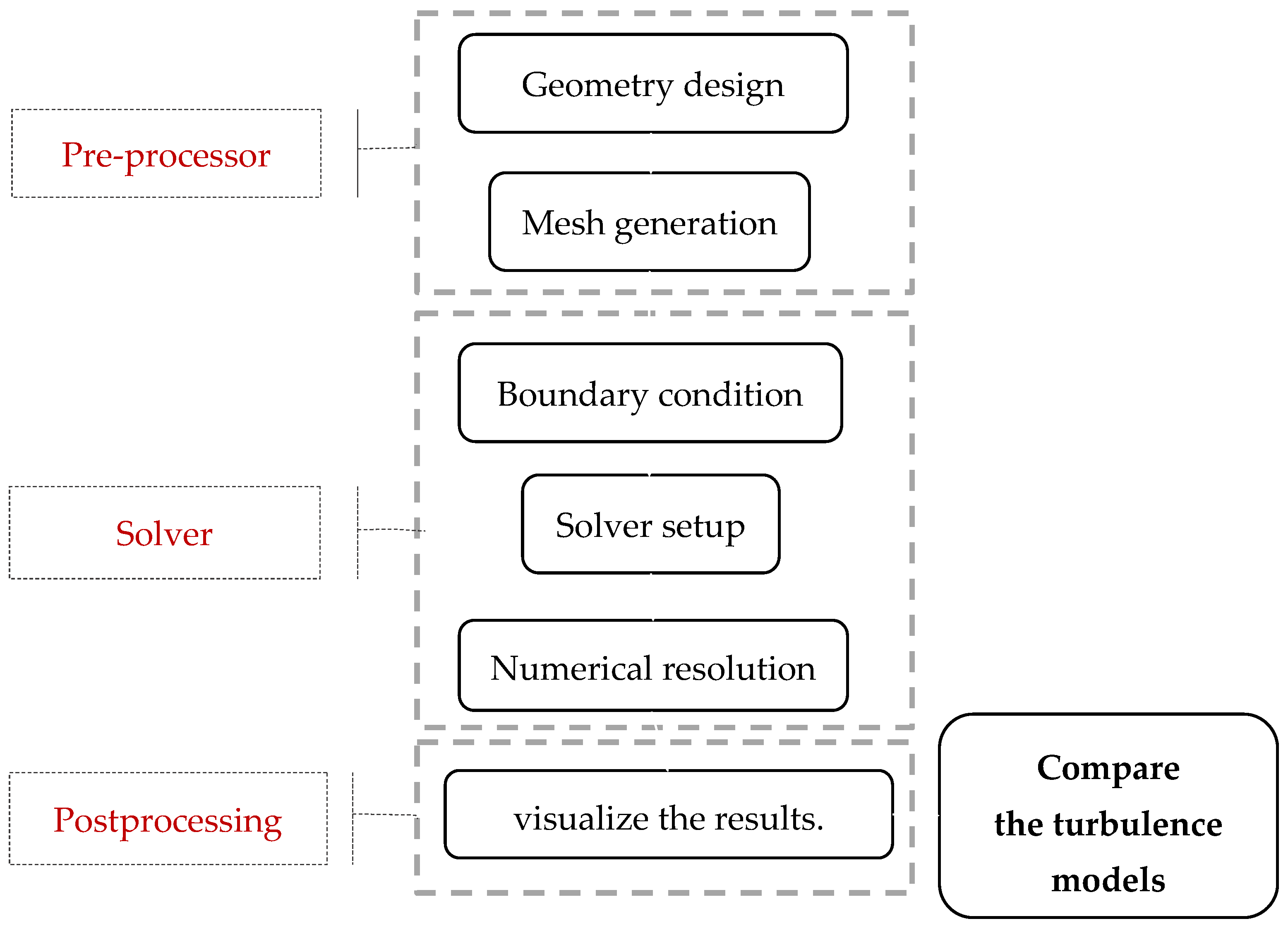
The exhaust manifold analysis process involves several critical steps, as outlined in Figure 1 (e.g., Bober et al. [18] and Tao et al. [19]). The first stage is preprocessing, wherein we create a geometric model of the manifold and gather relevant information such as dimensions, material properties, and operating conditions. Next, we mesh the model into a finite number of elements and refine the mesh to enhance its accuracy in specific areas of interest.
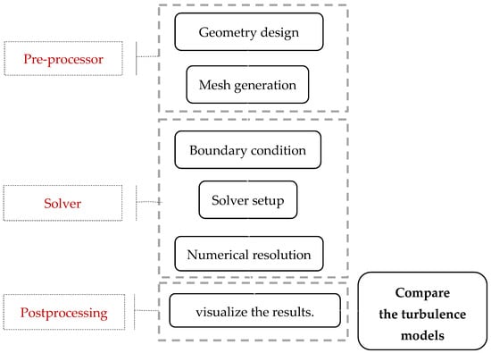
Figure 1.
Flowchart of modeling.
Our second step is the solver, whereby we solve the primary equations of fluid mechanics using numerical algorithms, considering the turbulence model used.
Finally, postprocessing entails visualizing and interpreting the CFD analysis results, including extracting relevant information like drag and lift coefficients, pressure distribution, and velocity profiles. To choose the best model, it is crucial to complete these steps with all the turbulence models examined to compare velocity distribution, pressure, turbulent kinetic energy, and temperature predictions.
2.2. Mathematical Modeling
Governing Equations
The three basic principles governing fluid motion are mass, momentum, and energy conservation (Sahoo and Tahiya [20], Teja et al. [21], and Benek and Ozsoyal [22]).
where:
ρ is the density, V is the fluid velocity vector, τij is the viscous stress tensor, p is the pressure, F represents the body forces, q is the heat source term, e is the internal energy, t is the time, ϕ is the dissipation term, and ∇.q is the heat loss by conductivity. Fourier’s law for heat transfer by conduction can be used to describe q, as follows:
The formula for thermal conductivity (k) involves temperature (T). One or more terms might be negligible, depending on the physics governing fluid motion.
In the simulations, the PISO algorithm was used for pressure velocity coupling to solve the equations for the flow field variable values in each computational cell. The discretization scheme used was a first-order upwind scheme, except for the pressure field, where the second-order upwind scheme was applied. The transient formulation utilized is bounded as second-order implicit.
2.3. Turbulence Models Equations
The provided table offers a comprehensive overview of the various turbulence models utilized in our research study (e.g., Rezaeiha et al. [23]). Each turbulence model is defined by the number of its governing equations, the presence or absence of transition modeling, and its respective abbreviation. Herein, there follows a brief elucidation of each model (Table 1).

Table 1.
Turbulence models overview.
2.3.1. The RNG K-ε Model
The k-ε turbulence model is widely used in CFD simulations. It is a two-equation model based on the Reynolds-averaged Navier–Stokes (RANS) equations.
The k-ε model consists of two transport equations: one is for turbulent kinetic energy (k) and one is for the dissipation rate of the turbulent kinetic energy (ε). The turbulent kinetic energy represents the kinetic energy associated with random fluctuations in velocity, while the dissipation rate represents the rate at which the turbulent kinetic energy is dissipated into thermal energy (Gao et al. [24]).
The k-ε model is widely recognized in the field of engineering for its simplicity and computational efficiency when dealing with turbulent flows. However, this model has been found to have limitations, particularly in the case of swirling flows, and its ability to accurately capture complex turbulent phenomena is questionable. As a result, advanced turbulence models, such as the large eddy simulation and direct numerical simulation, are sometimes employed to achieve more precise predictions. The judicious use of these models can lead to more accurate results in applications where precision is paramount (Ishihara et al. [25] and Deng et al. [26]):
and:
The following terms are of significance when describing different factors that contribute to the generation of turbulent kinetic energy:
- -
- Gk signifies the production of turbulent kinetic energy resulting from mean velocity gradients.
- -
- Gb denotes the generation of turbulent kinetic energy attributed to buoyancy.
- -
- YM represents the involvement of fluctuating dilatation in compressible turbulence, contributing to the overall dissipation rate.
- -
- αs and αk represent the reciprocal effective Prandtl numbers for ε and k, respectively.
- -
- Sk and Ss are designated as user-defined source terms.
The k-ε model assumes that the turbulent viscosity is proportional to the ratio of the turbulent kinetic energy to the dissipation rate. This relationship is expressed as:
where is the turbulent viscosity, is the density of the fluid, Cmu is a constant that is typically 0.09, k is the turbulent kinetic energy, and ε is the dissipation rate of turbulent kinetic energy.
2.3.2. SST K-ω Model
The SST k-omega turbulence model is a mathematical model used in CFD to simulate turbulent flows. It is a two-equation model that solves two turbulence-related variables, k (turbulent kinetic energy) and omega (specific dissipation rate) (e.g., Adanta et al. [27] and Costa et al. [28]).
Turbulent kinetic energy (k):
Specific dissipation rate (ω):
where:
Gω represents the generation of ω, Gk represents the generation of k due to mean velocity gradients.
τk and τω represent the effective diffusivity of k and ω, respectively.
Yω and Yk represent the dissipation of ω and k in the turbulence, while δω represents the cross-diffusion term.
Sk represents user-defined source terms.
The ω model addresses two transport equations for k and ω, along with the continuity, momentum, and energy equations. The transport equation for k covers the production, diffusion, and dissipation of turbulent kinetic energy, while the transport equation for omega deals with the production and destruction of the specific dissipation rate.
2.3.3. K-Kl- Transition Model
The k-kl-ω transition model, an extension of the standard k-ω model (e.g., Wang and Wang [29] and Salimipour [30]), introduces an extra transport equation for laminar kinetic energy (kl) in addition to the existing k-ω transport equations. This augmentation is designed to anticipate the initiation and span of transition by addressing low-frequency large-scale velocity fluctuations within the boundary layer. These fluctuations serve as indicators of pre-transition processes. The model considers both natural and bypass transitions. Unlike the TSST and SSTI models, the k-ω model relies more on physics-based principles rather than correlations.
Within this model, there exist transport equations for turbulent kinetic energy per unit mass (kT), laminar kinetic energy per unit mass (kL), and the specific dissipation rate (ω). When these differential equations are expressed in an incompressible form, they manifest as follows:
where P, RBP, RNAT, and D denote the turbulent production, bypass transition, natural transition, and near-wall dissipation term, respectively.
2.3.4. Transition SST Model
The SST k-ω transition model, also known as the model, introduces two additional transport equations for γ and , alongside the existing SST k-ω transport equations. This extension enhances the SST k-ω model’s capability to predict the onset and length of transition. The intermittency equation initiates local transition, while the momentum–thickness equation captures non-local flow effects, making the model sensitive to factors such as length scale, Re, pressure gradient, and freestream turbulence intensity6. Operating as a correlation-based model, it employs empirical correlations for to activate the model or identify those instances where transition may be bypassed due to exceptionally high turbulence levels. To predict free shear flows as fully turbulent, the SST k-ω model incorporates turbulent production limiters (e.g., Rajkumar et al. [31]) to prevent excessive turbulent kinetic energy predictions in stagnation regions.
This equation represents the intermittency equation factor (γ) in a turbulent flow. It includes the terms for production (Pγ), destruction (Eγ), and diffusion.
This equation represents the transport equation for the turbulent Reynolds number (Reθ) associated with thermal fluctuations. It includes the terms for production (Pθt) and diffusion.
2.3.5. Reynolds Stress Model
The transport equations for the transport of the Reynolds stresses, , can be written as follows (e.g., Jubaer et al. [32]):
The provided set of equations describes the conservation equations for turbulent flow. Several terms in these equations, namely, Cij, DL,ij, Pij, and Fij, do not necessitate any additional modeling. However, DT,ij, Gij, ϕij, and ϵij require modeling to complete the equations. The following sections elaborate on the modeling assumptions necessary to solve this set of equations.
3. Exhaust Manifold Analysis
3.1. Manifold Design
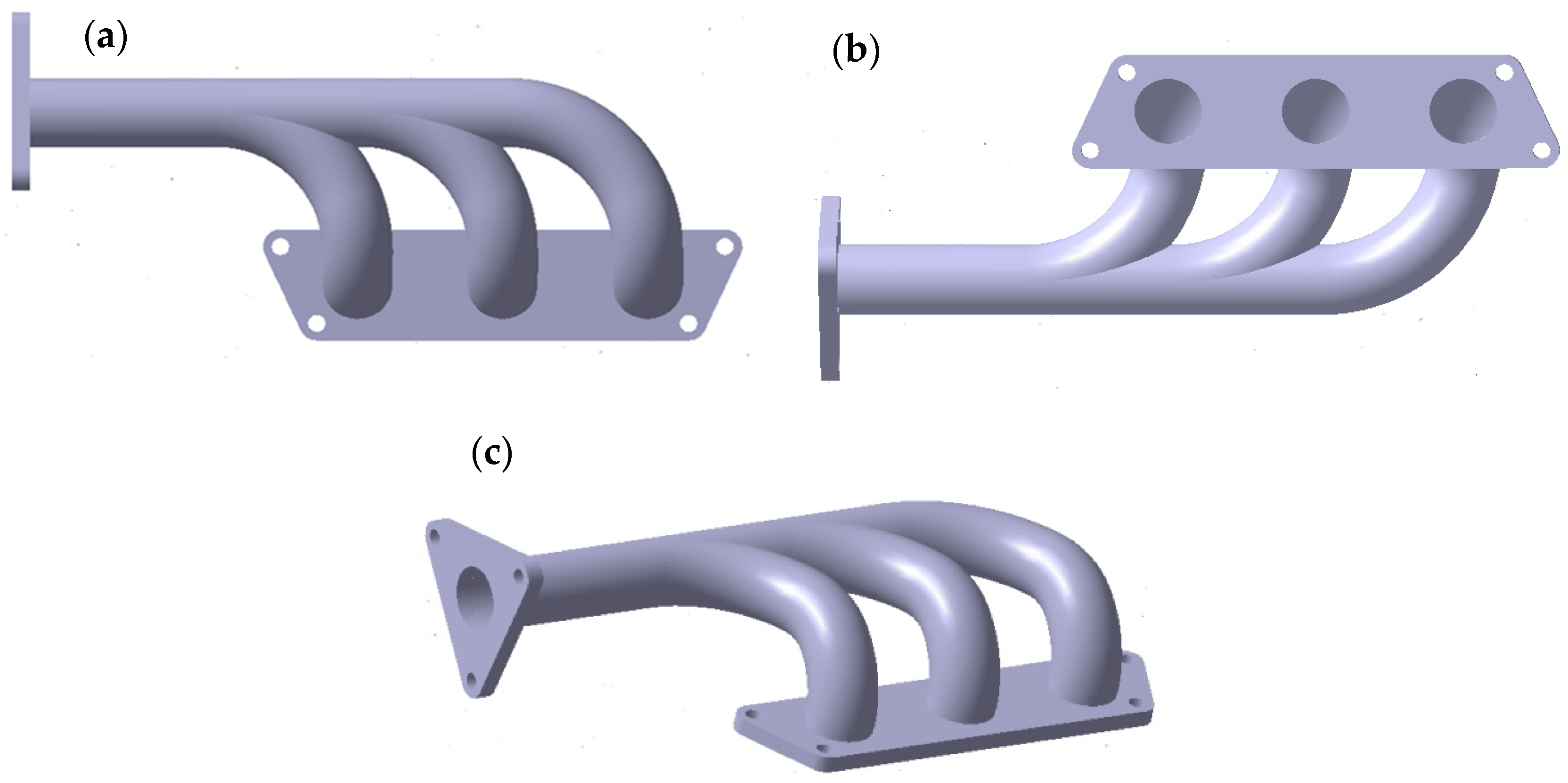
The system was modeled using CATIA V5 R21 software for part design. The CAD model of the exhaust manifold system can be seen in Figure 2 (e.g., Wu et al. [33]).

Figure 2.
(a) Top view of the exhaust manifold. (b) Bottom view of the exhaust manifold. (c) Isometrical view of the exhaust manifold.
3.2. Material Fluid Properties
Carbon-oxide-nitride is used in the CFD analysis of an exhaust manifold due to its unique properties, which make it suitable for modeling exhaust gases. With a density of 1 kg/m3, it accurately represents gases, indicating a low-density fluid that aligns well with the behavior of exhaust gases, which are less dense than liquids or solids. The specific heat capacity (Cp) is represented as a piecewise polynomial, enabling precise modeling of the variation in heat capacity with temperature. This is particularly important in exhaust systems, where gas temperature can vary significantly. The relatively low thermal conductivity of 0.0454 W/mK is consistent with the thermal properties of gases, which generally exhibit lower thermal conductivities compared to solids or liquids. The viscosity of 1.72 × 10⁻⁵ kg/m.s indicates a low-viscosity fluid, which is typical of gases, thereby facilitating the examination of flow dynamics in the exhaust manifold.
The specific heat capacity (Cp) can be mathematically expressed as a piecewise polynomial function of temperature. The model divides the temperature range into several segments, each represented by a polynomial of a specific degree:
where:
are the coefficients of the polynomial segments for each respective temperature range.
are the temperature breakpoints that define the range for each polynomial segment.
are the highest degrees of the polynomials in their respective segments.
For the given range from 300 K to 5000 K, the coefficients are defined as a1 = 560.0615, a2 = 1.755483, a3 = −0.001770155, a4 = 1.16292 × 10⁻⁶, and a5 = 3.775009 × 10⁻¹⁰.
These properties collectively facilitate a thorough analysis of the thermal and flow characteristics within the exhaust manifold, guaranteeing the precise capture of the gas’s compressibility and varying thermal behavior.
3.3. Boundary Condition
Conducting a comparative study of different turbulence models with consistent boundary conditions is crucial for a meaningful analysis to investigate how each turbulence model responds to different flow conditions. Some models may perform better in certain regimes (e.g., attached boundary layers or separated flows) than others.
Table 2 provides a comprehensive overview of the boundary conditions employed in our comparative study. These conditions were consistently applied across all turbulence models to facilitate a comprehensive evaluation. The specified boundary conditions encompass a velocity magnitude of 20 m/s for the three inlets of the exhaust manifold. Additionally, distinct inlet temperatures of 790 K, 800 K, and 810 K were designated for inlet 1, inlet 2, and inlet 3, respectively. Notably, all specified zones exhibit a hydraulic diameter of 0.06 m. This standardized methodology affords a meticulous assessment of turbulence model performance across a spectrum of flow scenarios. Convective heat transfer has been employed to represent the thermal interaction between the exhaust gas and the external environment. For this, a convective boundary condition is set (Malik et al. [34]), using Newton’s law of cooling:
where:
Table 2.
Boundary conditions.
h is the heat transfer coefficient of 40 W/m2K.
is the ambient temperature of 400 K.
The approach ensures that the simulation accurately depicts the heat exchange between the exhaust manifold walls and the surrounding air.
3.4. Grid Analysis and Mesh
An essential aspect of CFD simulations includes the careful determination of grid size. The grid must have sufficiently large dimensions to accurately represent the geometry, while also considering that a higher node count can result in longer CPU processing times. To determine the best mesh size for this analysis, a grid sensitivity study was implemented using eight different cell sizes, and two parameters were chosen to represent each grid: heat transfer and the velocity at the outlet. The study compared the changes in these parameters and their magnitudes at the exhaust gas outlet for the different mesh sizes, and the results showed that a grid size of 31,038 cells gave satisfactory results. Although a grid size of 109,668 also gave satisfactory results, it significantly increased the computational time. Therefore, a grid size of 31,038 cells was chosen for the simulation as it did not affect the results significantly. Table 3 shows the average velocity and maximum velocity for each grid and provides the percentage deviations from the chosen grid size.
Table 3.
Mesh convergence study.
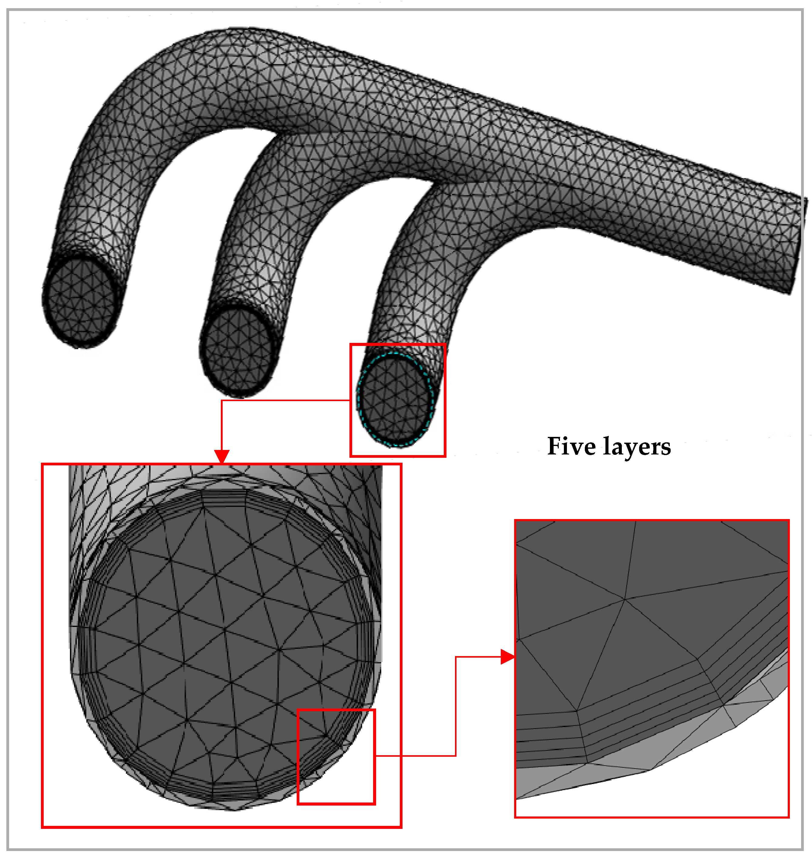
In near-wall regions, the solution gradients are very high, but accurate calculations are paramount to the success of the simulation. Since the calculations deal with solid-fluid variables, the near-wall treatment is essential. In Figure 3, mesh inflation is employed around the exhaust gas to ensure a y+ value of less than 1 throughout all simulations. An inflation mode with 5 layers is also used, adding extra layers of mesh cells near the solid boundaries where significant flow gradients are present (e.g., Ouyoussef et al. [35]). These layers are gradually refined toward the wall to provide better resolution of the boundary layer and to capture the flow phenomena in that region. This technique is commonly used in CFD simulations to achieve higher resolution when capturing near-wall flow behavior.
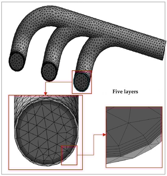
Figure 3.
Meshed exhaust manifold, inflation mode around the fluid.
3.5. Time Step
The Courant–Friedrichs–Lewy (CFL) condition ensures numerical stability. For explicit schemes, the CFL number remains less than 1. In our simulation, we opted for a CFL number of 0.5 for the initial estimation, to provide a margin of safety. The CFL condition is mathematically expressed as ; it is particularly critical for transient simulations involving compressible flows, most notably in exhaust manifold scenarios, where the flow characteristics change over time and need to be accurately captured. We considered a velocity magnitude v of 20 m/s and grid mesh of 0.01 m; as previously determined, the corresponding initial timestep was calculated as ∆t = 0.00025 s.
3.6. Results and Discussion
3.6.1. Temperature Comparison
Figure 4 reveals the distribution of the temperature at the outlet of the exhaust manifold using the five turbulence models; all models predict a similar maximum temperature at the outlet, showing that the maximum at the outlet of the exhaust manifold is closely clustered between 807.73 K and 808.58 K, with the k-kl-ω model predicting the highest maximum temperature at 808.58 K. Minimum temperatures vary more, ranging from 790.23 K to 795.56 K, with the Reynolds stress model showing the lowest minimum temperature at 790.23 K. The k-kl-ω model stands out, presenting the broadest temperature range.
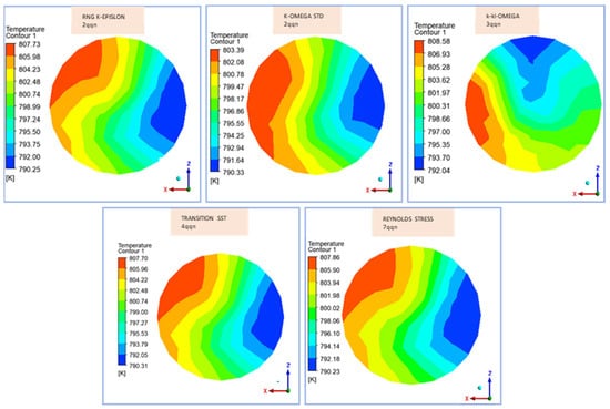
Figure 4.
Temperature distribution at the outlet of the exhaust manifold (90 s).
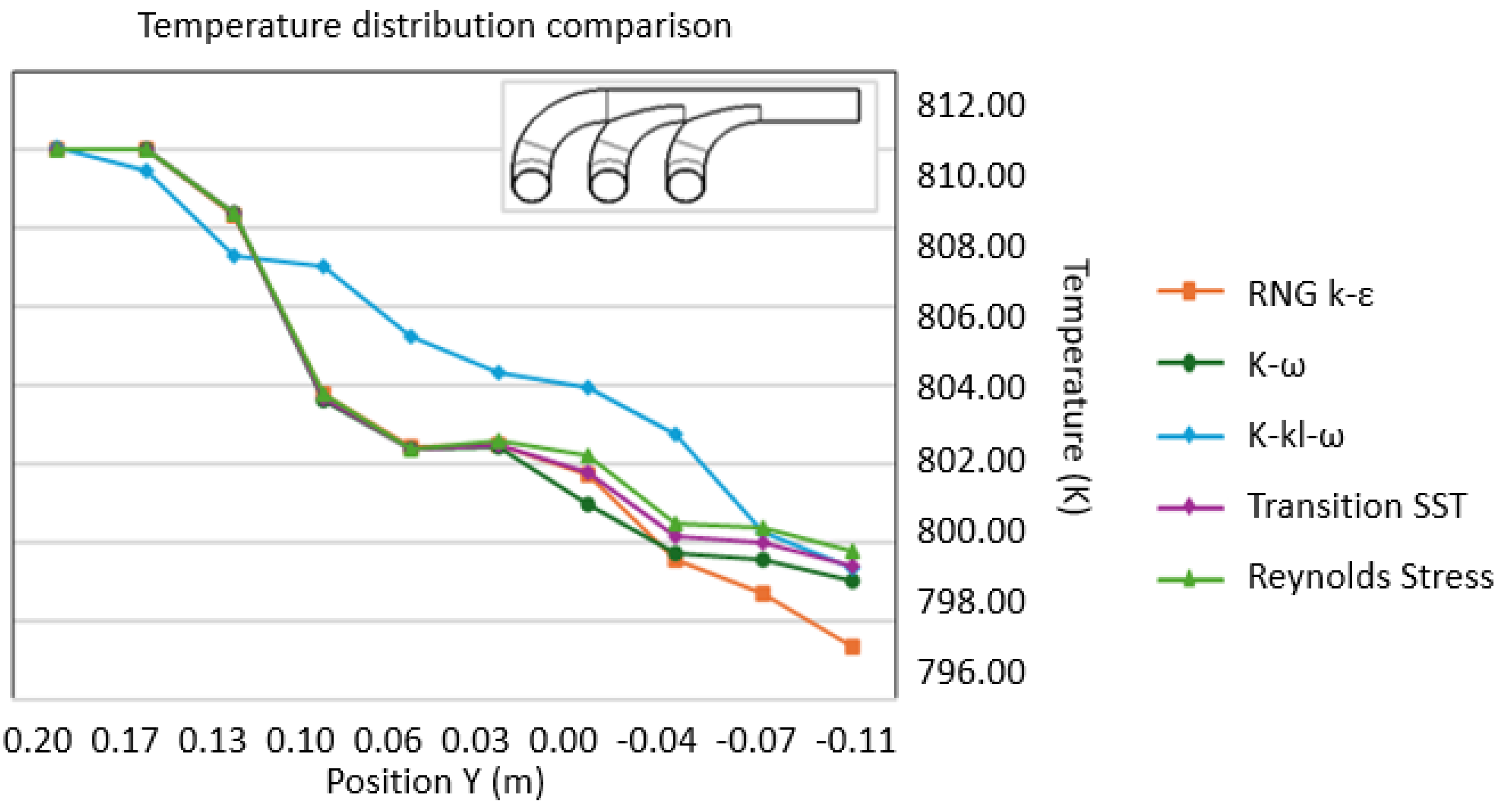
All models show a decreasing temperature trend as the position Y changes from the inlet 0.20 m to the outlet −0.11 m, as shown in Figure 5; k-kl-ω shows the highest temperatures initially, reflecting sensitivity to transitional flows. The RNG k-epsilon model shows a rapid temperature decrease, reaching the lowest minimum temperature, around 798 K, at −0.11 m. K-omega STD and k-kl-ω models display similar trends, with k-kl-ω consistently predicting higher temperatures. The transition SST and Reynolds stress models exhibit closely matched trends, with transition SST initially showing slightly higher temperatures.
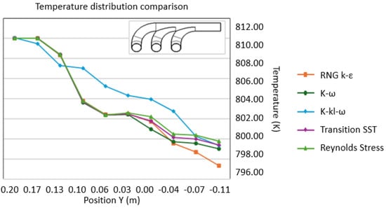
Figure 5.
Temperature distribution comparison.
As depicted in the 2D ZY plane in Figure 6, the temperature distribution among the exhaust manifold shows the contours for different turbulence models—RNG k-epsilon, k-omega STD, k-kl-ω, transition SST, and Reynolds stress. Each model illustrates a gradient from high to low temperatures, with the highest temperatures generally observed near the inlet and the lowest temperatures towards the outlet. The k-kl-ω model predicts the highest maximum temperature of 808.58 K, indicating its sensitivity to transitional flow effects. The RNG k-epsilon model shows a rapid decrease in temperature, with the lowest minimum temperatures around 790 K. K-omega STD and k-kl-ω exhibit similar trends, while the transition SST and Reynolds stress models show closely matched distributions. These findings are essential for understanding the thermal behavior of the exhaust manifold, aiding in optimizing design and material selection to enhance performance and durability.
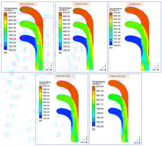
Figure 6.
Temperature distribution among the exhaust manifold (100 s).
3.6.2. Velocity Comparison
Figure 7 depicts the velocity profiles at the exhaust manifold outlet in the ZX plane. The k-kl-ω model indicates the presence of the highest velocity regions, reaching up to 80.63 m/s, signifying strong transitional flow effects. In contrast, the RNG k-epsilon, k-omega STD, transition SST, and Reynolds stress models exhibit maximum velocities in the 63–65 m/s range. These discrepancies in velocity profiles underscore the distinct capabilities of each model in accurately capturing flow dynamics.
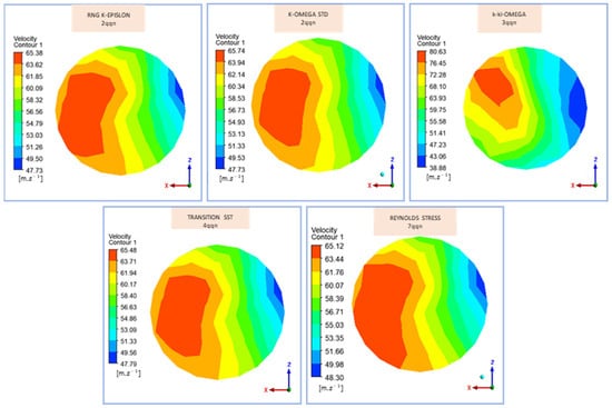
Figure 7.
Velocity distribution at the outlet of the exhaust manifold (60 s).
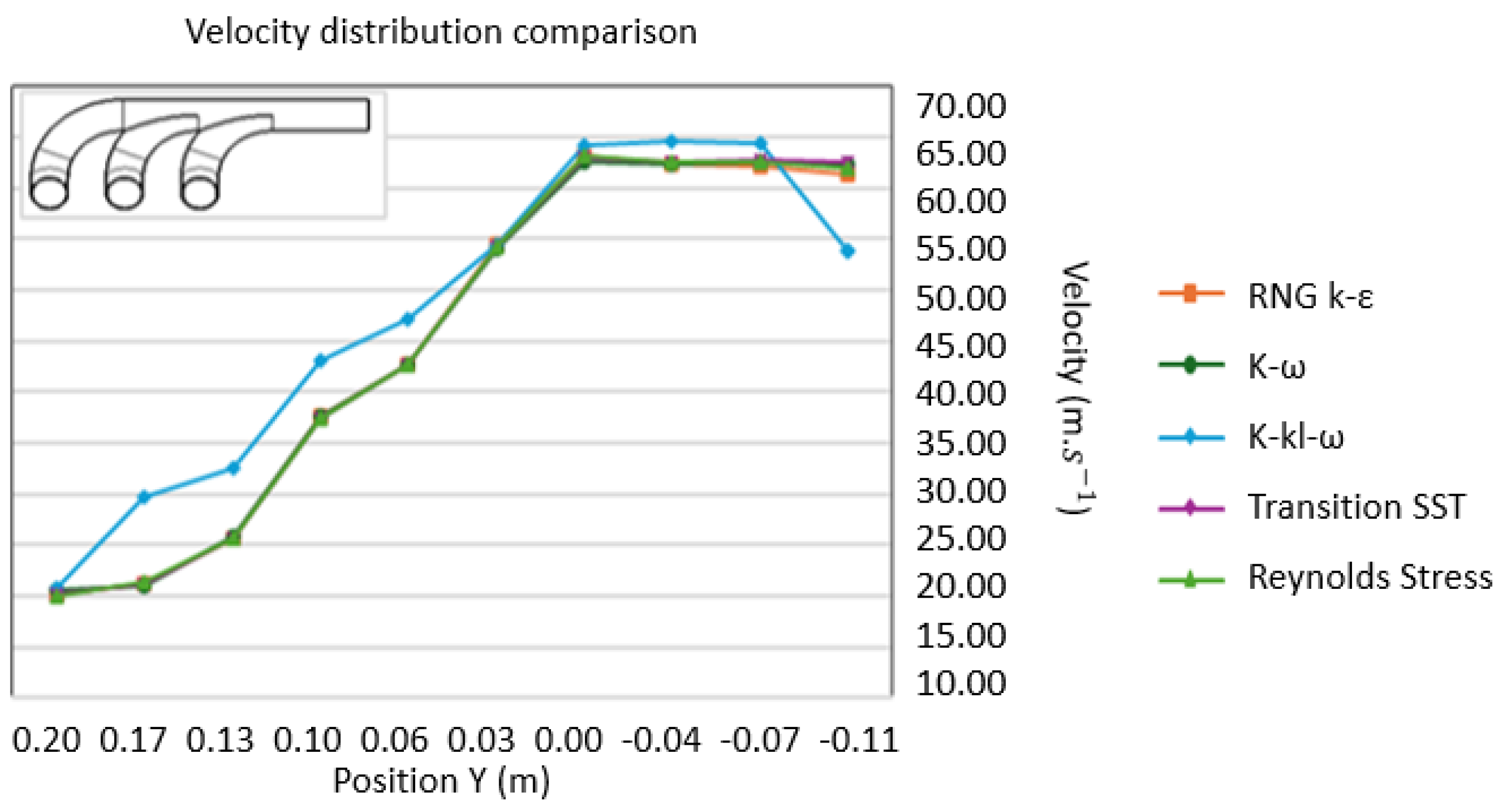
The diagram shown in Figure 8 illustrates how velocity varies across the manifold, with positions ranging from 0.2 m to −0.105 m in the XZ plane. Initially, the velocity at the three inlets is set to 20 m/s as per the boundary condition. As it moves through the exhaust manifold, the velocity gradually increases. The k-kl-ω model stands out with higher velocities, peaking at around 65 m/s and maintaining higher velocities along the exhaust path y-axis; the RNG k-epsilon, k-omega STD, transition SST, and Reynolds stress models exhibit similar peak velocities, at around 63–65 m/s.
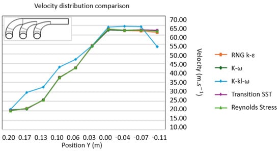
Figure 8.
Velocity distribution in the exhaust manifold.
These models predict slightly lower peak velocities compared to the k-kl-ω model but follow a nearly identical trend, increasing steadily up to 0.00 m and then maintaining or slightly decreasing.
Although all models follow a similar curve in the velocity distribution graph, despite varying peak values, it highlights their general agreement in predicting flow behavior within the exhaust manifold. This consistency across different turbulence models indicates reliable modeling of the exhaust flow dynamics, which is crucial for optimizing the manifold’s design for efficient exhaust gas expulsion and for minimizing backpressure. The k-kl-ω model’s higher-velocity predictions provide additional insights into transitional flow effects, offering a more detailed analysis for fine-tuning manifold performance.
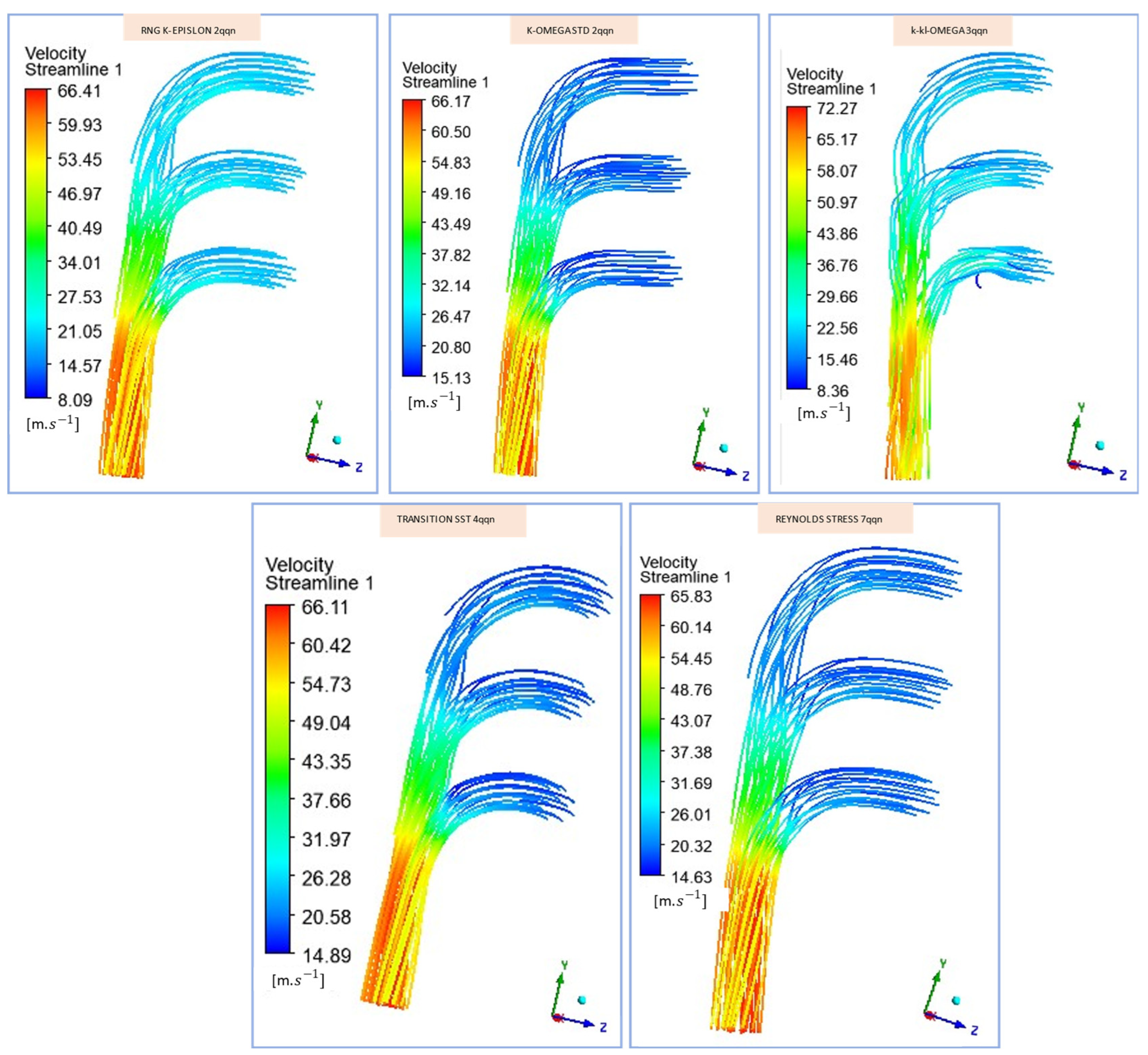
As can be seen, Figure 9 depicts the contour of the streamlined velocity contours across the exhaust manifold, captured for various turbulence models, revealing that all models predict a similar trend in flow patterns with smooth streamlines. The k-kl-ω model predicts the highest velocities (up to 72.27 m/s) and exhibits more complex patterns, effectively capturing transitional flow effects. In contrast, the other models (RNG k-epsilon, k-omega STD, transition SST, and Reynolds stress) show slightly lower maximum velocities (around 65–66 m/s) but maintain well-structured and consistent flow patterns. The k-kl-ω turbulence model uses the length scale variable, which enhances its capability to handle the flows with the manifold while considering the curvature of the inlets. This feature allows the model to represent the domain’s exhaust gases and turbulent structures accurately.

Figure 9.
Velocity distribution across the exhaust manifold (70 s).
3.6.3. Pressure Comparison
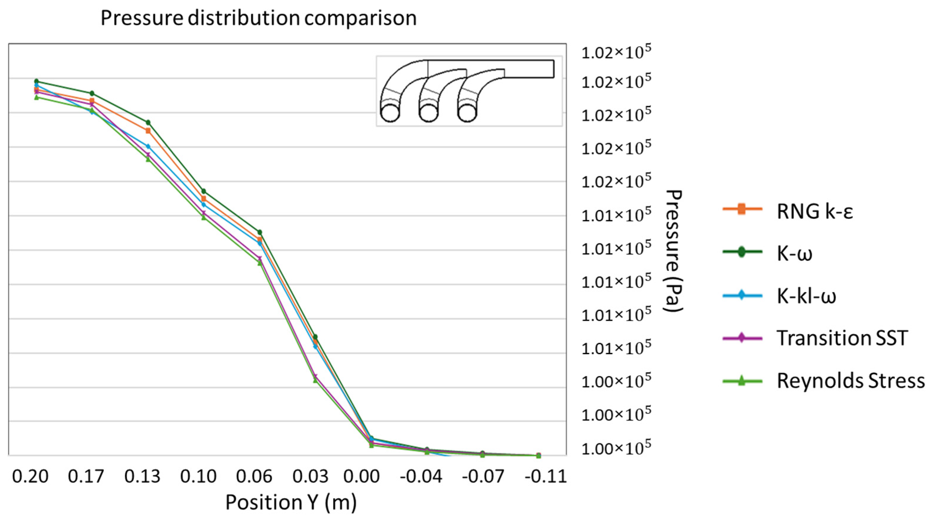
The following diagram presents the pressure fluctuations observed over a spatial range spanning from 0.2 m to −0.105 m.
The Figure 10 shows that the exhaust manifold indicates a consistent trend in pressure drop for all turbulence models. The pressure decreases steadily from around 1.02 × 10⁵ Pa at 0.20 m to the defined outlet pressure of 105 Pa at −0.11 m. However, a distinct pressure increase is observed near the midpoint of the exhaust manifold (around 0 m); for all the models, there is a brief increase in pressure followed by a decline. This localized pressure increase suggests a potential point where the flow converges or where it faces resistance within the manifold. This pattern is consistently observed across all models. While there are minor discrepancies, the pressure curves for all models closely align, indicating reliable predictions of the pressure distribution.
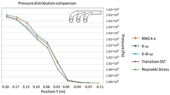
Figure 10.
Pressure drops from the inlet of the manifold.
3.6.4. Turbulent Kinetic Energy Comparison
The diagram shown in Figure 11 represents the evolution of turbulent kinetic energy (TKE) along the length of the exhaust manifold for various turbulence models, progressing from the inlet to the outlet.
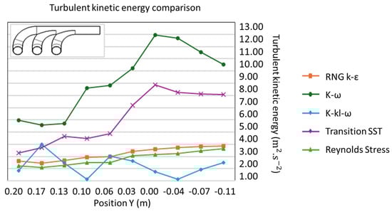
Figure 11.
Turbulent kinetic energy comparison.
Among the simulations, it is noteworthy that both the turbulence models of transition SST and k-ω exhibit distinctive behavior, showcasing the maximum TKE in the range [8,9,10,11,12] m2.s−2, suggesting its contribution to heightened turbulence levels, particularly in the latter part of the manifold. In contrast, the k-kl-ω, Reynolds stress, and RNG k-epsilon models display lower TKE values, generally ranging between 0 and 4 m2/s2, suggesting a more subdued turbulence prediction. The higher TKE values observed in the k-omega and transition SST models can be attributed to their advanced turbulence modeling approaches, which are designed to capture the complexities of transitional and turbulent flows more accurately. These models include additional mechanisms to account for turbulent energy transfer and dissipation, leading to higher predicted TKE levels. One possible explanation for the notably more significant turbulent kinetic energy (TKE) that is predicted by the transition SST is that it employs a hybrid approach that combines elements of the k-ω and k-ε turbulence models. This combination allows for a more comprehensive representation of turbulence phenomena, particularly in transitional flow regimes, which may enhance TKE predictions.
3.6.5. Discussion
The following table summarizes the results of a comparative analysis of the various turbulence models employed in simulating fluid flow within an exhaust manifold. The parameters examined included velocity (ms−2), temperature (K), pressure (Pa), and TKE (m2s−2).
In Table 4, we have presented a consistent synthesis of our simulation results for the five turbulence models. Each turbulence model depicts variations in these parameters across the manifold (y-axis position). The k-kl-ω model predicts the highest maximum velocity at 64.599 m/s, suggesting that using the length scale variable of this turbulence model helps to handle transitional flows more efficiently, reflected in the wider velocity range. Conversely, we found that the Reynolds stress and k-ω turbulence models give the lowest maximum velocity at 62 m/s, reflecting their detailed and conservative approaches to turbulence modeling. Temperature projections are consistent among the exhaust manifold, with all models showing maximum temperatures of around 810 K and slight variations in minimum temperatures, indicating accurate thermal behavior capture. Pressure predictions show minor differences, with the k-kl-ω model predicting a slightly lower minimum pressure and the k-omega STD model predicting the highest maximum pressure. The most significant differences are observed in the TKE values, with the k-omega STD and SST transition models predicting significantly higher TKE, indicating heightened turbulence levels, particularly in the latter part of the manifold. These insights are crucial for optimizing exhaust manifold design to ensure efficient exhaust flow, minimize pressure losses, and accurately predict the thermal and flow dynamics within the system.
Table 4.
Turbulence model comparison.
4. Conclusions and Perspective
A transient CFD analysis of an exhaust manifold was performed using five different turbulence models. The objective was to compare and analyze the performance of these models in predicting key flow parameters to identify the most accurate models for capturing flow characteristics.
Mesh independency, temporal discretization, and the characteristics of different turbulence models were systematically evaluated. After determining optimal simulation parameters, the models were compared under consistent conditions to ensure a fair result.
The k-kl-ω model gave the highest maximum velocity and exhibited the widest temperature range, underlining its advanced capability to capture transitional flow effects using the length scale variable, which enhances its ability to handle the flows with the manifold, considering the curvature of the inlets. The k-ω STD and SST transition models presented notably higher TKE values, denoting their advanced capabilities in modeling complex turbulent and transitional flows. These models regularly predicted heightened turbulence levels, particularly in the latter part of the manifold. Conversely, the Reynolds stress and RNG k-epsilon models displayed lower TKE values, suggesting a more subdued turbulence prediction. Despite these differences, all models exhibited similar trends in pressure drop, with a noticeable increase near the midpoint of the manifold, suggesting a common point of flow convergence or resistance.
Comparing simulation results to experimental data is essential for thoroughly assessing their veracity. This will serve as a benchmark for testing the precision and reliability of each turbulence model when analyzing the complexities of fluid flow within the exhaust manifold.
Author Contributions
Conceptualization, O.N. and M.H.; Methodology, O.N., M.H., M.L.S. and L.J.; Software, O.N. and M.H.; Validation, O.N. and M.H.; Formal analysis, O.N., M.H. and M.L.S.; Investigation, O.N., M.H. and M.L.S.; Resources, O.N., M.H., M.L.S. and L.J.; Data curation, O.N., M.H. and M.L.S.; Writing—original draft, O.N. and M.H.; Writing—review & editing, M.L.S. and L.J.; Visualization, M.L.S. and L.J.; Supervision, L.J.; Project administration, M.L.S. and L.J.; Funding acquisition, M.L.S. and L.J. All authors have read and agreed to the published version of the manuscript.
Funding
The APC was founded by Transilvania University of Brasov.
Institutional Review Board Statement
Not applicable.
Informed Consent Statement
Not applicable.
Data Availability Statement
No new data were created or analyzed in this study.
Conflicts of Interest
The authors declare no conflict of interest.
References
- Soares, A.; Martins, R.F.; Mateus, A.F.R. Structural integrity analyses of two gas turbines exhaust systems used for naval propulsion. Procedia Struct. Integr. 2017, 5, 640–646. [Google Scholar] [CrossRef]
- Chen, M.; Wang, Y.; Wu, W.; Xin, J. Design of the Exhaust Manifold of a Turbo Charged Gasoline Engine Based on a Transient Thermal Mechanical Analysis Approach. SAE Int. J. Engines 2015, 8, 75–81. [Google Scholar] [CrossRef]
- Chaudhari, S.G.; Borse, P.N.; Patil, R.Y. Experimental and CFD Analysis of Exhaust Manifold to Improve Performance of IC Engine. Int. Res. J. Eng. Technol. 2017, 4, 1598–1602. [Google Scholar]
- Wang, D.; Zhang, W.; Liu, D.; Chen, X.; Tang, G.; Okosun, T.; Wu, B.; Zhou, C.Q. CFD Simulation of a 6-Cylinder Diesel Engine Intake and Exhaust Manifold. In ASME International Mechanical Engineering Congress and Exposition; American Society of Mechanical Engineers: New York, NY, USA, 2015; Volume 57472, p. V07BT09A034. [Google Scholar]
- Cihan, Ö.; Bulut, M. CFD analysis of exhaust manifold for different designs. Eur. Mech. Sci. 2019, 3, 147–152. [Google Scholar] [CrossRef]
- Bral, P.; Tripathi, J.P.; Dewangan, S.; Mahato, A.C. CFD analysis of an exhaust manifold for emission reduction. Mater. Today Proc. 2022, 63, 354–361. [Google Scholar] [CrossRef]
- Zhou, H.; Ye, J. On the selection of turbulent model for the nearshore hydrodynamics modeling of coral reefs: Insight from an inter-comparison study. Ocean. Eng. 2022, 266, 113046. [Google Scholar] [CrossRef]
- Ajayi, O.O.; Unser, L.; Ojo, J.O. Implicit rule for the application of the 2-parameters RANS turbulence models to solve flow problems around wind turbine rotor profiles. Clean. Eng. Technol. 2023, 13, 100609. [Google Scholar] [CrossRef]
- Cen, Z.L. A Comparative Study of Omega RSM and RNG k–ε Model for the Numerical Simulation of a Hydrocyclone. Iran. J. Chem. Chem. Eng. 2014, 33, 53–61. [Google Scholar]
- Huang, H.; Sun, T.; Zhang, G.; Li, D.; Wei, H. Evaluation of a developed SST k-ω turbulence model for the prediction of turbulent slot jet impingement heat transfer. Int. J. Heat Mass Transf. 2019, 139, 700–712. [Google Scholar] [CrossRef]
- Cabello, R.; Popescu, A.E.P.; Bonet-Ruiz, J. Heat transfer in pipes with twisted tapes: CFD simulations and validation. Comput. Chem. Eng. 2022, 166, 107971. [Google Scholar] [CrossRef]
- Eroglu, S.; Duman, I.; Ergenc, A.; Yanarocak, R. Thermal Analysis of Heavy Duty Engine Exhaust Manifold Using cfd (No. 2016-01-0648); SAE Technical Paper; SAE International: Warrendale, PA, USA, 2016. [Google Scholar]
- Moen, A.; Mauri, L.; Narasimhamurthy, V.D. Comparison of k-ε models in gaseous release and dispersion simulations using the CFD code FLACS. Process Saf. Environ. Prot. 2019, 130, 306–316. [Google Scholar] [CrossRef]
- Allawi, M.K.; Oudah, M.H.; Mejbel, M.K. Analysis of exhaust manifold of spark-ignition engine by using computational fluid dynamics (CFD). J. Mech. Eng. Res. Dev 2019, 42, 211–215. [Google Scholar] [CrossRef]
- Bajpai, K.; Chandrakar, A.; Agrawal, A.; Shekhar, S. CFD analysis of exhaust manifold of SI engine and comparison of back pressure using alternative fuels. IOSR J. Mech. Civ. Eng. 2017, 14, 23–29. [Google Scholar] [CrossRef]
- Blocken, B.; van Druenen, T.; Toparlar, Y.; Malizia, F.; Mannion, P.; Andrianne, T.; Marchal, T.; Maas, G.-J.; Diepens, J. Aerodynamic drag in cycling pelotons: New insights by CFD simulation and wind tunnel testing. J. Wind Eng. Ind. Aerodyn. 2018, 179, 319–337. [Google Scholar] [CrossRef]
- Sunny Manohar, D.; Krishnaraj, J. Modeling and Analysis of Exhaust Manifold using CFD. IOP Conf. Ser. Mater. Sci. Eng. 2018, 455, 012132. [Google Scholar] [CrossRef]
- Bober, B.; Andrych-Zalewska, M.; Boguś, P. Influence of exhaust manifold modification on engine power. Combust. Engines 2024, 196, 54–65. [Google Scholar] [CrossRef]
- Tao, Z.; Cheng, Z.; Zhu, J.; Li, H. Effect of turbulence models on predicting convective heat transfer to hydrocarbon fuel at supercritical pressure. Chin. J. Aeronaut. 2016, 29, 1247–1261. [Google Scholar] [CrossRef]
- Sahoo, D.K.; Thiya, R. Coupled CFD–FE analysis for the exhaust manifold to reduce stress of a direct injection-diesel engine. Int. J. Ambient Energy 2019, 40, 361–366. [Google Scholar] [CrossRef]
- Teja, M.A.; Ayyappa, K.; Katam, S.; Anusha, P. Analysis of exhaust manifold using computational fluid dynamics. Fluid Mech. Open Acc. 2016, 3, 1000129. [Google Scholar]
- Benek, G.; Ozsoysal, O.A. Influences of the dead end on the flow characteristics at the exhaust manifold of a marine diesel engine. J. Therm. Eng. 2021, 7, 1519–1530. [Google Scholar] [CrossRef]
- Rezaeiha, A.; Montazeri, H.; Blocken, B. On the accuracy of turbulence models for CFD simulations of vertical axis wind turbines. Energy 2019, 180, 838–857. [Google Scholar] [CrossRef]
- Gao, F.; Wang, H.; Wang, H. Comparison of different turbulence models in simulating unsteady flow. Procedia Eng. 2017, 205, 3970–3977. [Google Scholar] [CrossRef]
- Ishihara, T.; Qian, G.W.; Qi, Y.H. Numerical study of turbulent flow fields in urban areas using modified k−ε model and large eddy simulation. J. Wind Eng. Ind. Aerodyn. 2020, 206, 104333. [Google Scholar] [CrossRef]
- Deng, Y.; Feng, J.; Wan, F.; Shen, X.; Xu, B. Evaluation of the turbulence model influence on the numerical simulation of cavitating flow with emphasis on temperature effect. Processes 2020, 8, 997. [Google Scholar] [CrossRef]
- Adanta, D.; Fattah, I.R.; Muhammad, N.M. Comparison of standard k-epsilon and SST k-omega turbulence model for breastshot waterwheel simulation. J. Mech. Sci. Eng. 2020, 7, 39–44. [Google Scholar] [CrossRef]
- Costa, L.M.F.; Montiel, J.E.S.; Correa, L.; Lofrano, F.C.; Nakao, O.S.; Kurokawa, F.A. Influence of standard k-ε, SST κ-ω and LES turbulence models on the numerical assessment of a suspension bridge deck aerodynamic behavior. J. Braz. Soc. Mech. Sci. Eng. 2022, 44, 350. [Google Scholar] [CrossRef]
- Wang, J.; Wang, Y. Assessment of turbulence models and mesh types for the simulation of multi-body separation by coupling the CFD and rigid body dynamics. J. Phys. Conf. Ser. 2023, 2512, 012005. [Google Scholar] [CrossRef]
- Salimipour, E. A modification of the k-kL-ω turbulence model for simulation of short and long separation bubbles. Comput. Fluids 2019, 181, 67–76. [Google Scholar] [CrossRef]
- Rajkumar, R.A.B.; Raffic, N.M.; Babu, D.K.G.; Vignesh, V. Comparative Study on Effective Turbulence Model for NACA0012 Airfoil using Spalart–Allmaras as a Benchmark. Int. J. Trend Sci. Res. Dev. 2020, 4, 1049–1056. [Google Scholar]
- Jubaer, H.; Afshar, S.; Xiao, J.; Chen, X.D.; Selomulya, C.; Woo, M.W. On the effect of turbulence models on CFD simulations of a counter-current spray drying process. Chem. Eng. Res. Des. 2019, 141, 592–607. [Google Scholar] [CrossRef]
- Wu, J.; Xiao, H.; Sun, R.; Wang, Q. Reynolds-averaged Navier–Stokes equations with explicit data-driven Reynolds stress closure can be ill-conditioned. J. Fluid Mech. 2019, 869, 553–586. [Google Scholar] [CrossRef]
- Malik, R.; Khan, M.; Munir, A.; Khan, W.A. Flow and heat transfer in Sisko fluid with convective boundary condition. PLoS ONE 2014, 9, e107989. [Google Scholar] [CrossRef] [PubMed]
- Nouhaila, O.; Hassane, M. Analyzing the Impact of Cracks on Exhaust Manifold Performance: A Computational Fluid Dynamics Study. Int. J. Heat Technol. 2024, 42, 475. [Google Scholar] [CrossRef]


Disclaimer/Publisher’s Note: The statements, opinions and data contained in all publications are solely those of the individual author(s) and contributor(s) and not of MDPI and/or the editor(s). MDPI and/or the editor(s) disclaim responsibility for any injury to people or property resulting from any ideas, methods, instructions or products referred to in the content. |
© 2024 by the authors. Licensee MDPI, Basel, Switzerland. This article is an open access article distributed under the terms and conditions of the Creative Commons Attribution (CC BY) license (https://creativecommons.org/licenses/by/4.0/).