Article

Neural Robust Control for a Mobile Agent Leader–Follower System

by
David Rodriguez-Castellanos
*,
Marco Blas-Valdez
,
Gualberto Solis-Perales
and
Marco Antonio Perez-Cisneros
Computational Sciences Department, Centro Universitario de Ciencias Exactas e Ingenierias (CUCEI), University of Guadalajara, 1421 Marcelino García Barragán Blvd., Guadalajara 44430, Jalisco, Mexico
*
Author to whom correspondence should be addressed.
Appl. Sci. 2024, 14(13), 5374; https://doi.org/10.3390/app14135374
Submission received: 2 May 2024 / Revised: 24 May 2024 / Accepted: 28 May 2024 / Published: 21 June 2024
(This article belongs to the Special Issue Intelligent Control of Dynamical Processes and Systems)

Abstract

:
A controller employing a combined new strategy of output feedback linearization and a recurrent high-order neural network (RHONN) adaptive approach for a mobile agent leader–follower system is presented. The controller structure is based on feedback linearization; then, a scheme of lumping uncertainties which are estimated via the RHONN is incorporated; with this estimate, the controller is able to produce a robust control action for mobile agents so they track a prescribed reference trajectory. Moreover, the nonlinear system part is transformed into a linearizable one; then, a specific function lumps all the nonlinearities, uncertain parameters, and unmodeled dynamics of the system; this overall function is estimated via the RHONN. Thus, both parametric uncertainties and unmodeled dynamics between agents can be compensated via the controller, and, subsequently, follower agents track the reference provided by the leader. The obtained controller is such that the estimation scheme is not based on high-gain controllers. Here, it is underlined that the main contribution consists of designing a nonlinear controller and combining it with an RHONN to estimate the nonlinear uncertainties in the leader–follower system. This control action includes robust features provided by the online recurrence and the nonlinear base of the neural network in which not general but specific parametric disturbances and unmodeled discrepancies are identified or compensated. For this control scheme, only nominal values of the system parameters are required, as well as the velocities of the agents. Numeric simulation of the model and designed tracking control are carried out in which the control law is applied to a two-wheeled differential mobile robot model, obtaining satisfactory results for tracking angular velocities of the wheels.

1. Introduction

The study and development of autonomous mobile robots have increased in recent years due to their wide range of potential applications and new integration of technologies to improve them. Additionally, multirobot systems have made significant progress in terms of coordination and cooperation, becoming increasingly important in everyday life cooperative implementations [1,2]. Multiple agents can solve tasks faster and at lower cost if they work cooperatively, in contrast to a single robot trying to perform the same task. On this subject, the leader–follower strategy is the most commonly used methodology in the formation control of multirobot systems [3,4,5].
One of the major challenges in dealing with control and automation of any dynamical system, and in particular with control of differential robots, when the tracking control problem is addressed is the management of the model uncertainties and parameter variations.
Differential mobile robots are widely used because of their minimal resource requirements in design and construction, as well as their ability to maneuver to any position using straight lines, curves, or by rotating on their own axis. However, these are systems that have a large number of parameters that are generally uncertain and exhibit model discrepancies, external disturbances, and parameter uncertainties. These previously mentioned issues must be tackled through a well-suited control system design. Significant results have been obtained in this particular subject, for instance, in [6], a controller was suggested for a differential mobile robot, which utilizes recursive integral back-stepping to track and stabilize the trajectory of robots. Such a controller requires complete knowledge of all parameters and states. In [7], a hybrid controller was proposed that combines a kinematic controller based on a neural network and an adaptive control reference model. The controller parameters are adapted online using the neural network, and by tuning the adaptive kinematic controller, rapid convergence to the desired trajectory is achieved. Moreover, the adaptive reference control model maintains the desired tracking performance when parameters and state uncertainties occur. In [8], a PID controller was used for controlling the angular velocity of the wheels, and in [9], the dynamics of the parameters of the robot were controlled using two PID control blocks. Nevertheless, both cases are limited by the precision of the robot model. In [6], recursive back-stepping control was implemented with good results in semiglobal regions. In [10], a discrete-time case was stated and a recurrent high-order neural network was trained with an extended Kalman filter algorithm to identify the whole state, not just parameters, as we propose. Unlike the works mentioned so far, our approach to this problem combines an adaptable and robust parameter estimation with output feedback linearization control.
It is not uncommon for linearization methodologies to be applied in designing nonlinear control systems; the main idea is to partially or fully transform the nonlinear dynamics of the system to be controlled into linearized dynamics, thus being able to apply the known linear control techniques at an operating point [11]. This method has a significant number of limitations: it cannot be used for all kind of systems; the complete state must be measured; and it does not guarantee robustness in the presence of unstructured uncertainties or unmodeled dynamics. In this sense, there are results in which the number of states to be known can be reduced, and, furthermore, the nonlinear dynamics can be estimated so that the controller may counteract them. This is considered robust control, as reported in [12,13].
Robustness and adaptation against system uncertainties are essential in control system design. Recurrent neural networks have been widely used as an adaptive model for classification, pattern recognition, identification, optimization, and processing [14,15,16]. They are mainly based on the Hopfield model [17]. These kind of networks are considered good candidates for nonlinear system applications that face uncertainties, and they are attractive due to their easy implementation, relatively simple structure, robustness, and ability to adjust their parameters online [18,19,20,21]. These networks may estimate uncertain nonlinear functions solely based on velocity measurements. The main idea for this work is to implement a linearizing controller which has access to these aforementioned uncertain estimates to compensate them in the system. In other words, the controller will compensate or attenuate the effect of parametric variations, model errors, and disturbances; this derives high-order recurrent neural network properties.
Frequently, in control system design, full-state measurement is difficult to obtain, and reliable velocity measurements are needed in order to eliminate tachometers and numerical differentiation but maintain high control accuracy. One option is to use joint velocity observers. The concept of the model-based observer was tailored to estimate manipulator joint velocities in [22], ensuring local asymptotic stability. In [23], neural networks were used for closed-loop output feedback control without joint velocity measurements. Only the inertia matrix was assumed to be known; a neural network observer was designed to estimate the unknown velocity. In [24], a multilayer perceptron model control was presented that was based on full-state identification. However, it lacked recurrence adaptability properties, and nonlinear structures were not included in the identification process. In the mentioned research papers, observers have been proposed, which assume an exact knowledge of the dynamics of manipulator parameters. For the adaptive control approach, linearity in the unknown parameters is required; therefore, the exact knowledge of the robot dynamics is necessary to be successful. Generally, this cannot be achieved in practice.
In this work, the goal consists of designing a nonlinear robust adaptive controller called neuro-robust control to track the angular velocities of both wheels of a differential mobile robot in a leader–follower configuration. We assume that there is no more information of the systems other than the velocity outputs and a nominal value of some parameters. Thus, the desired trajectory is parameterized in the Cartesian plane with the angular velocities of right and left wheels. A system composed of two parts is proposed: the design of a linearizing controller and an estimator with a high-order neural network. The robustness of the RHONN approach is analyzed in [14]. This aspect of our approach offers both online adaptability and nonlinear combined features, contributing to the novelty of this paper.
The paper is organized as follows. The next section presents the materials and methods. Section 3 contains the main contribution, consisting of the neuro-robust controller design. In Section 4, the results of the neuro-robust control applied to the differential robots are discussed. Finally, in Section 5, the discussion and conclusions are provided.

2. Materials and Methods

The controller introduced in this study, named neuro-robust control, comes from the nonlinear geometrical control theory [11] and the theory for recurrent high-order neural networks [14]. The first part consists of determining a diffeomorphic transformation such that the nonlinear system can be transformed into a linearizable system via a nonlinear controller. Once the system is linearizable, the linearizing control requires at least the knowledge of two nonlinear functions: one of them is obtained from the nominal parameter values of the system, whereas the other function contains the dynamic of the nonlinear model, including parameters. In this sense, the controller must have this information in order to be counteracted; however, it is not possible. Instead, an estimate of these dynamics is constructed using a recurrent high-order neural network. This estimate is carried out without the use of high-gain estimators, as was reported in [12,13]. Therefore, in coming subsections, the tools used to design the neuro-robust controller are described.

2.1. Exact State Feedback Linearization

Let us consider a multiple-input and multiple-output system, given as follows, which could describe the dynamics of the mobile agent:
x ˙ = f ( x ) + i = 1 m g i ( x ) u i , y 1 = h 1 ( x ) , y m = h m ( x ) .
where f ( x ) , g 1 ( x ) , , g m ( x ) : U U ; U R n is defined as an open set of continuously differentiable vector fields; h 1 ( x ) , , h m ( x ) are smooth real-valued functions also defined on U, which determine the outputs of the system.
The starting point of the analysis is a multivariable version of the relative degree notion. The relative degree ( r i ) is exactly the number of times that the ith output needs to be differentiated (evaluated at x = x 0 ) for at least one component of the input vector to appear explicitly. A multivariable nonlinear system of the form (1) has a relative degree vector ρ = [ r 1 , , r m ] at a point x 0 if
  • L g j L f k h i ( x ) = 0 , for all 1 j m , k < r i 1 and for all x in a neighborhood of x 0 .
  • The following m × m matrix:
    A ˜ ( x ) = L g 1 L f r 1 1 h 1 ( x ) L g m L f r 1 1 h 1 ( x ) L g 1 L f r 2 1 h 2 ( x ) L g m L f r 2 1 h 2 ( x ) L g 1 L f r m 1 h m ( x ) L g m L f r m 1 h m ( x )
    is nonsingular at x 0 .
Consider for simplicity that previous conditions are satisfied and the system has a relative degree vector [ r 1 , r 2 , , r m ] at x o (considering an equal number of inputs and outputs; thus, m = n ), with sum r = r 1 + + r m exactly equal to n; therefore, there exist n functions such that they define a mapping as Φ ( x ) = z 1 1 ( x ) , , z r 1 1 ( x ) , , z 1 m ( x ) , , z r m m ( x ) T , where z 1 i ( x ) = h i ( x ) , z 2 i ( x ) = L f h i ( x ) ,⋯, z r i i ( x ) = L f r i 1 h i ( x ) , i = 0 , 1 , , n , this mapping has a nonsingular Jacobian at x o and then is considered as a local coordinate transformation at a neighborhood of x o . Now, differentiating with respect to time, the following canonical system form is obtained:
z ˙ 1 i = z 2 i , z ˙ 2 i = z 3 i , z ˙ r i 1 i = z r i i , z ˙ r i i = b i ( z ) + j = 1 m a i j ( z ) u j , y i = z 1 i ,
where
a i j ( z ) = L g j L f r i 1 h i ( Φ 1 ( z ) ) f o r 1 i , j m ,
b i ( z ) = L f r i h i ( Φ 1 ( z ) ) f o r 1 i m ,
where x = Φ 1 ( z ) is the inverse mapping of transformation matrix, the functions a i j ( z ) are exactly the entries of the matrix (2), and b i ( z ) are the entries of the vector given by b ( z ) = [ L f r 1 h 1 , L f r 2 h 2 , , L f r m h m ] T . System (3) with functions (4) and (5) defines a fully linearizable system via feedback. Now, the next step is to design a control feedback that leads the outputs of the system to a prescribed trajectory y R ( t ) [11]; to this end, the tracking control feedback is given as follows:
u i = A 1 ( z ) b i ( z ) + y R ( r ) i = 1 r c i 1 e ( i 1 ) ( t ) ,
where c i , , c i 1 are real numbers, and e ( i 1 ) ( t ) = y ( i 1 ) ( t ) y R ( i 1 ) ( t ) is the error between the ( i 1 ) th time derivative of the real output and the ( i 1 ) th time derivative of the output reference. It is noticeable that the elements of the matrix A 1 ( z ) are those mentioned in Equation (4); moreover, the matrix A 1 ( z ) is the same as the relative degree inverse matrix A ˜ ( Φ 1 ( z ) ) in Equation (2), that is, A 1 ( z ) = A ˜ ( Φ 1 ( z ) ) . Therefore, under the local effect of control law of the form (6), the system (1) follows the desired signal y R ( t ) ; this is the tracking error that can be led to zero as t approaches infinity.
The control law (6) is the so-called perfect or exact control strategy and it is impractical since it requires the perfect knowledge of the matrix A ˜ ( Φ 1 ( z ) ) , the functions b i ( z ) , and the full state vector. Therefore, to tackle this problem, an estimator for the unknown functions and states is designed such that the tracking control makes the system trajectories follow the prescribed reference; this requires only the measure of the output. Such an estimate can be realized by means of recurrent high-order neural network.

2.2. Recurrent High-Order Neural Networks Estimation

Let us consider a neural network with n neurons and m inputs for our estimation purposes. The state of each neuron is governed by a differential equation of the following form:
x i ˙ = λ i x i + μ i k = 1 L w i k j I k y j d j ( k ) ,
where x i is the state of the ith neuron; L is the number of high-order product terms; { I 1 , I 2 , , I L } is a collection of L unordered subsets of { 1 , 2 , , m + n } ; λ i , μ i > 0 , i = 1 , 2 , , n are real coefficients; w i k are the adjustable real coefficients of the neural network; d j ( k ) are non-negative integers; and y is a vector constructed from the inputs to each neuron, defined as
y = y 1 y n y n + 1 y n + m = S ( x 1 ) S ( x n ) S ( u 1 ) S ( u m ) ,
where u = [ u 1 u 2 u m ] T is the vector of external inputs to the neural network. The function S ( ) is a smooth, monotonically increasing sigmoid [14].
We define a vector of dimension L as follows:
ζ = ζ 1 ζ 2 ζ L = j I 1 y j d j ( 1 ) j I 2 y j d j ( 2 ) j I L y j d j ( L )
and thus, (7) can be expressed as follows:
x ˙ i = λ i x i + μ i k = 1 L w i k ζ k .
If the weight vector is defined as w i = μ i [ w i 1 w i 2 w i L ] T , then (10) can be written as
x ˙ i = λ i x i + w i T ζ .
Therefore, the RHONN model takes the following form:
x ˙ = Λ x + W T ζ ,
where x = [ x 1 x n ] T R n ; W = [ w 1 , w 2 , , w n ] T R n × L and Λ = d i a g ( λ 1 , λ 2 , , λ n ) R n × n , and it is assumed that λ i > 0 .
Consider the identification problem of a nonlinear dynamic system of the form
χ ˙ = F ( χ , u ) ,
where χ R n is the vector state of the system, u R m is the system input, and F : R n + m R n is a smooth vector field defined on a compact set γ R n + m . It was shown in [25] that the model (12) can approximate suitably any system of the form (13) as long as the number of connections L is selected adequately [26].
Assuming that the system (13) and the model (12) are initialized at the same state x ( 0 ) = χ ( 0 ) , then for any ε > 0 and any finite T > 0 , there exists an integer L and a matrix W R L × n such that the state x ( t ) of the modeled RHONN in (12) with L high-order connections and weights W = W satisfies
sup 0 t T | x ( t ) χ ( t ) | ε .
The weights w i , for i = 1 , 2 , , n , are adjusted according to the learning law:
w ˙ i = Γ i ζ e i ,
where e i : = x i χ i is the error between the state of the network and the state to be identified, ζ is defined as in (9); and Γ i is a positive definite matrix. In the special case where Γ i = γ i I , where γ i > 0 is a scalar, then Γ i in (15) might be replaced by γ i [14].

3. Neuro-Robust Control

In this section, the main contribution is presented following the control scheme in Figure 1.
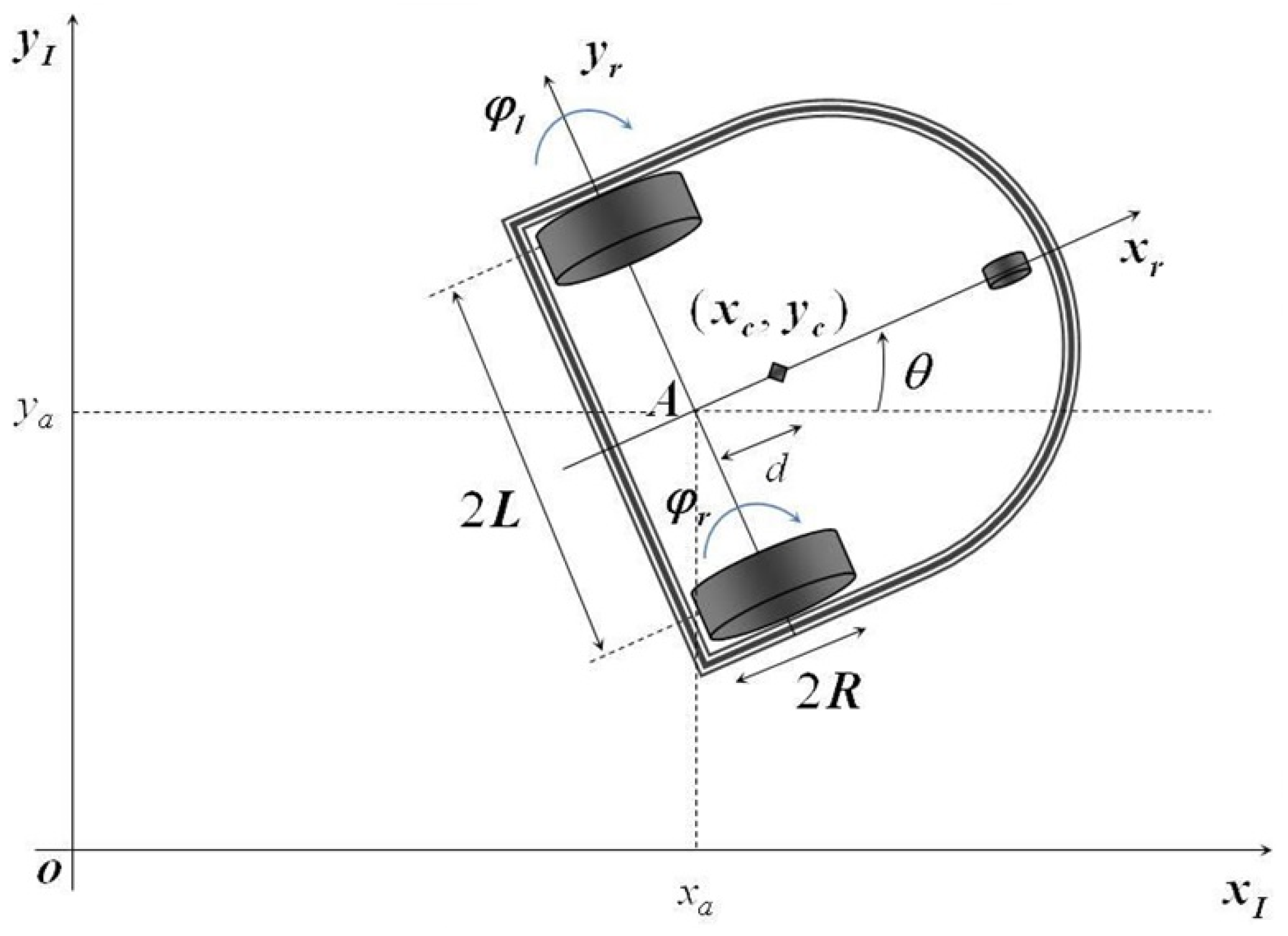
First, we define the dynamic model of a differential mobile robot. In Figure 2, we can observe the diagram of the differential mobile robot, and its dynamic model is
ω ˙ R ω ˙ L = m 1 V ω L ( ω L ω R ) m 1 2 m 2 2 + m 2 V ω R ( ω L ω R ) m 1 2 m 2 2 m 2 V ω L ( ω L ω R ) m 1 2 m 2 2 m 1 V ω R ( ω L ω R ) m 1 2 m 2 2 + m 1 R ( m 1 2 m 2 2 ) m 2 R ( m 1 2 m 2 2 ) τ R + m 2 R ( m 1 2 m 2 2 ) m 1 R ( m 1 2 m 2 2 ) τ L ,
m 1 = R ( M d 2 + J ) 4 L 2 + M R 4 , m 2 = R ( M d 2 + J ) 4 L 2 + M R 4 , V = M d R 2 4 L 2 .
The former equations are derived from the Newton–Euler approach and those were taken from [27]. Equation (16) shows the dynamic model selected to be analyzed. Each symbol represents the following:
  • M is the total mass of the differential mobile robot.
  • R is the radius of the wheel.
  • d is the distance from the wheel axle center to the center of mass.
  • J is the moment of inertia of the differential mobile robot about the vertical axis z through the center of mass.
  • L is the distance from the center of the robot to the wheel axis.
  • ω R and ω L are the angular velocities of the right and left wheels, respectively.
  • ω R d and ω L d are the desired angular velocities of the right and left wheels, respectively.

3.1. Controller Design

Applying the results presented in the previous section, we obtain the relative degree matrix given by
A ( x ) = m 1 R ( m 1 2 m 2 2 ) m 2 R ( m 1 2 m 2 2 ) m 2 R ( m 1 2 m 2 2 ) m 1 R ( m 1 2 m 2 2 ) ,
where the r a n k ( A ( x ) ) = 2 and d e t ( A ( x ) ) 0 , and
b ( x ) = m 1 v ω L ( ω L ω R ) m 1 2 m 2 2 + m 2 v ω R ( ω L ω R ) m 1 2 m 2 2 m 2 v ω L ( ω L ω R ) m 1 2 m 2 2 m 1 v ω R ( ω L ω R ) m 1 2 m 2 2 .
Then, we have the next local coordinate transformation as described in Section 2; Equations (3)–(5):
z 1 1 = h 1 ( x ) z 2 1 = b 1 + a 11 u 1 + a 12 u 2 z 1 2 = h 2 ( x ) z 2 2 = b 2 + a 21 u 1 + a 22 u 2 ,
where the linearized states are defined as z 1 1 = w R and z 1 2 = w L in Equation (16). Finally, the transformed system is as follows:
z ˙ 1 1 = m 1 v z 1 2 ( z 1 2 z 1 1 ) m 1 2 m 2 2 + m 2 v z 1 1 ( z 1 2 z 1 1 ) m 1 2 m 2 2 b 1 + m 1 R ( m 1 2 m 2 2 ) a 11 u 1 m 2 R ( m 1 2 m 2 2 ) a 12 u 2 ,
z ˙ 1 2 = m 2 v z 1 2 ( z 1 2 z 1 1 ) m 1 2 m 2 2 m 1 v z 1 1 ( z 1 2 z 1 1 ) m 1 2 m 2 2 b 2 m 2 R ( m 1 2 m 2 2 ) a 21 u 1 + m 1 R ( m 1 2 m 2 2 ) a 22 u 2 .
The control law for asymptotic trajectory tracking is given by Equation (6), where y R ( r ) represents the r-th derivative of the reference angular velocity for each wheel. The nonlinear functions denoted as b 1 ( z ) and b 2 ( z ) in (21) and (22) are uncertain and need to be estimated for the controller to compensate them. An RHONN is proposed to estimate these functions. The system takes the following form:
z ˙ 1 1 = b 1 ( z ) e s t i m a t e d + a 11 ( z ) u 1 + a 12 ( z ) u 2 , z ˙ 1 2 = b 2 ( z ) e s t i m a t e d + a 21 ( z ) u 1 + a 22 ( z ) u 2 .
In Equations (21) and (22), the terms a 11 , a 12 , a 21 , and a 22 do not depend on the states and are therefore constant. Additionally, note that these terms depend on the system parameters, but it is sufficient to know their signs and a nominal value. In actuality, there is no need to estimate them; it is sufficient for the controller to know their nominal value.
Hence, the matrix A takes the following constant form:
A = δ 1 δ 2 δ 3 δ 4 ,
where all δ i are positive. Then, the following control law using the estimated parameters by RHONN is obtained:
u 1 = δ 2 ( b 2 ^ ω L d ( r ) + e ω L k 2 ) δ 1 δ 4 δ 2 δ 3 δ 4 ( b 1 ^ ω R d ( r ) + e ω R k 1 ) δ 1 δ 4 δ 2 δ 3 ,
u 2 = δ 1 ( b 2 ^ ω L d ( r ) + e ω L k 2 ) δ 1 δ 4 δ 2 δ 3 δ 3 ( b 1 ^ ω R d ( r ) + e ω R k 1 ) δ 1 δ 4 δ 2 δ 3 ,
where e ω L = ω L ω L d and e ω R = ω R ω R d . The previous process was only described for a single mobile agent; for the leader–follower system, it is necessary to duplicate the procedure for the follower agent.
By estimating the parameter b, we eliminate certain restrictions of the exact linearization method, such as the requirement of knowing the complete state. This estimation ensures robustness, in the sense that the RHONN will adapt the function if any parameter changes its value. Note that the function b contains the varying parameters and model functions, and to generate the control law, it is sufficient to estimate the dynamic behavior of the function b rather than each parameter of the model.
Using (11) to identify (20), the model to be implemented is as follows:
z ^ ˙ 1 1 = λ 1 z ^ 1 1 + w 1 T ζ I ( z , u ) , z ^ ˙ 1 2 = λ 2 z ^ 1 2 + w 2 T ζ I ( z , u ) , z ^ ˙ 2 1 = λ 3 z ^ 2 1 + w 3 T ζ I ( z , u ) , z ^ ˙ 2 2 = λ 4 z ^ 2 2 + w 4 T ζ I ( z , u ) .
Then, a four-state RHONN is proposed to identify the states of the transformed system (21) and (22) for both the leader robot ( z 1 1 and z 1 2 ) and the follower robot ( z 2 1 and z 2 2 ). The parameters b 11 and b 12 are derived from the difference between z ^ ˙ 1 1 and z ^ ˙ 2 1 (which completely estimates (21)) and the known input parameter elements which can be denoted as A u . This is
b ^ 1 ( z ) = z ^ ˙ 1 1 a 11 ( z ) u 1 a 12 ( z ) u 2 , b ^ 2 ( z ) = z ^ ˙ 1 2 a 21 ( z ) u 1 a 22 ( z ) u 2 .
Finally, the weight adaptation law applied for each state is given by (15).

3.2. Stability Analysis

From (27), the RHONN identifier for the unknown parameters, taking into account input control and modeling error, can be rewritten as
z ^ ˙ = Λ z ^ ( t ) + W ζ ( z ( t ) ) + ν e r ( t ) ,
where ν e r ( t ) R n is the modeling error, and W R n × L is a matrix with values of the online estimated neural network weights, which minimizes ν e r ( t ) .
We define trajectory tracking error and identification error, respectively, as
z e ( t ) = z ( t ) z r ( t ) ,
e ( t ) = z ( t ) z ^ ( t ) .
Assumption 1 [18]. For every w i j W , a bounded set, the system (29) is bounded for every bounded state z ^ .
Assumption 2 [18]. There exist unknown constant weights W L such that the plant (21) and (22) is described without modeling error, by the neural network of the form
z ˙ ( t ) = Λ z ( t ) + W ζ ( z ( t ) ) .
In (32), we consider z ˙ ( t ) z ^ ˙ ( t ) . In order to analyze the error dynamics between the identified and the linearized system, we first obtain the identification error from (32) and (27) as in [14]
e ˙ ( t ) = z ˙ ( t ) z ^ ˙ ( t ) = Λ e ( t ) + W ˜ ζ ( z ( t ) ) ,
where W ˜ = W W .
As in [14], the weight adaptation law is selected as
t r W ˜ ˙ T W ˜ = γ e ( t ) T W ˜ ζ ( z ( t ) ) ,
which can be written element by element as
w ˙ i , j = γ e ( t ) T ζ j ( z ( t ) ) i = 1 , 2 , , n j = 1 , 2 , , L .
The adaptation law (35) guarantees that e ˙ ( t ) 0 as t , and also W ˜ ( t ) 0 as t .
On the other hand, we can write the expression for the derivative of the trajectory tracking error:
z ˙ e ( t ) = z ˙ ( t ) z ˙ r ( t ) Λ z e ( t ) + W ˜ r ζ ( z e ( t ) ) + u ,
where W ˜ r = W W r . Now, we are prepared to demonstrate asymptotic stability.
Theorem 1. 
For the linearized parametric system (21) and (22) under Assumptions 1 and 2, using the online learning control laws (25) and (26) the tracking error (36) is asymptotically stable at z e ( t ) = 0 .
Proof. 
The trajectory tracking problem for (23) reduces to a stabilization problem for (36), where the dynamics of identification error are included. Note that [ z e ( t ) , e ( t ) , W ˜ ] = [ 0 , 0 , 0 ] is an equilibrium point of the undisturbed autonomous system. For stability analysis, the candidate Lyapunov function is defined as
V T = 1 2 z e ( t ) 2 + 1 2 e ( t ) 2 + 1 2 t r { W ˜ T W ˜ } ,
which fulfills the needed characteristics of radially unbounded and V ( 0 ) = 0 of Barbashin–Krasovskii theorem [28], so that we demonstrate regulation for each of the three error dynamics (trajectory tracking error, identification error, and weight matrix error). The time derivative of (37) along the trajectories of (36) is
V ˙ T = λ z e ( t ) 2 + z e ( t ) T W ˜ r ζ ( z e ( t ) ) + z e ( t ) T u λ e ( t ) 2 + e ( t ) T W ˜ ζ ( z ( t ) ) + t r { W ˜ ˙ T W ˜ } .
Then, we substitute the learning law (34) with γ = 2 into (38) and make a change of variable from (31) to obtain
V ˙ T = λ z e ( t ) 2 + z e ( t ) T W ˜ r ζ ( z e ( t ) ) + z e ( t ) T u λ e ( t ) 2 + e ( t ) T W ˜ ζ ( e ( t ) + z r ( t ) ) e ( t ) T W ˜ ζ ( e ( t ) + z r ( t ) ) = λ z e ( t ) 2 + z e ( t ) T W ˜ r ζ ( z e ( t ) ) + z e ( t ) T u λ e ( t ) 2 .
Now, if we factorize the elements on the right-hand side of (39),
V ˙ T λ [ z e ( t ) 2 + e ( t ) 2 ] + z e ( t ) T [ W ˜ r ζ ( z e ( t ) ) + u ] .
If we prove that the right-hand side of (40) is negative, V T is decreasing and bounded from below by V T ( 0 ) . Thus, directly from Assumption 1, (25) and (26), one can conclude that z e ( t ) , w r i j ( t ) , u L 1 , where L 1 is the space of Lebesgue integrable functions; this means that weights remain bounded. Now, let us consider that we select gains in (25) and (26), guaranteeing that δ 1 δ 4 > δ 2 δ 3 such that W ˜ r ζ ( z e ( t ) ) u , then negative definiteness of V ˙ T is ensured. Thus, with the proposed control law, asymptotic stability for the error dynamics is proved by the Barbashin–Krasovskii theorem [28], ensuring the trajectory tracking to the reference signal for the linearized parametric system. □

4. Results

For simulation purposes, we consider a desired trajectory of a Lissajous curve in the plane, which needed to be parameterized into corresponding angular velocities ω R and ω L for both wheels using the kinematic model referenced in [27].
The trajectory was simulated for a time lapse of 60 s. For different periods, the model is under different disturbances and parametric variations. In between 10 and 20 s, the robot experiences an extra weight input, resulting in a 100% variation, as shown in Table 1 [29]. During the interval of 30 to 40 s, the system receives an external disturbance (a step of amplitude 7.5 rad/s) that accelerates only the right wheel.
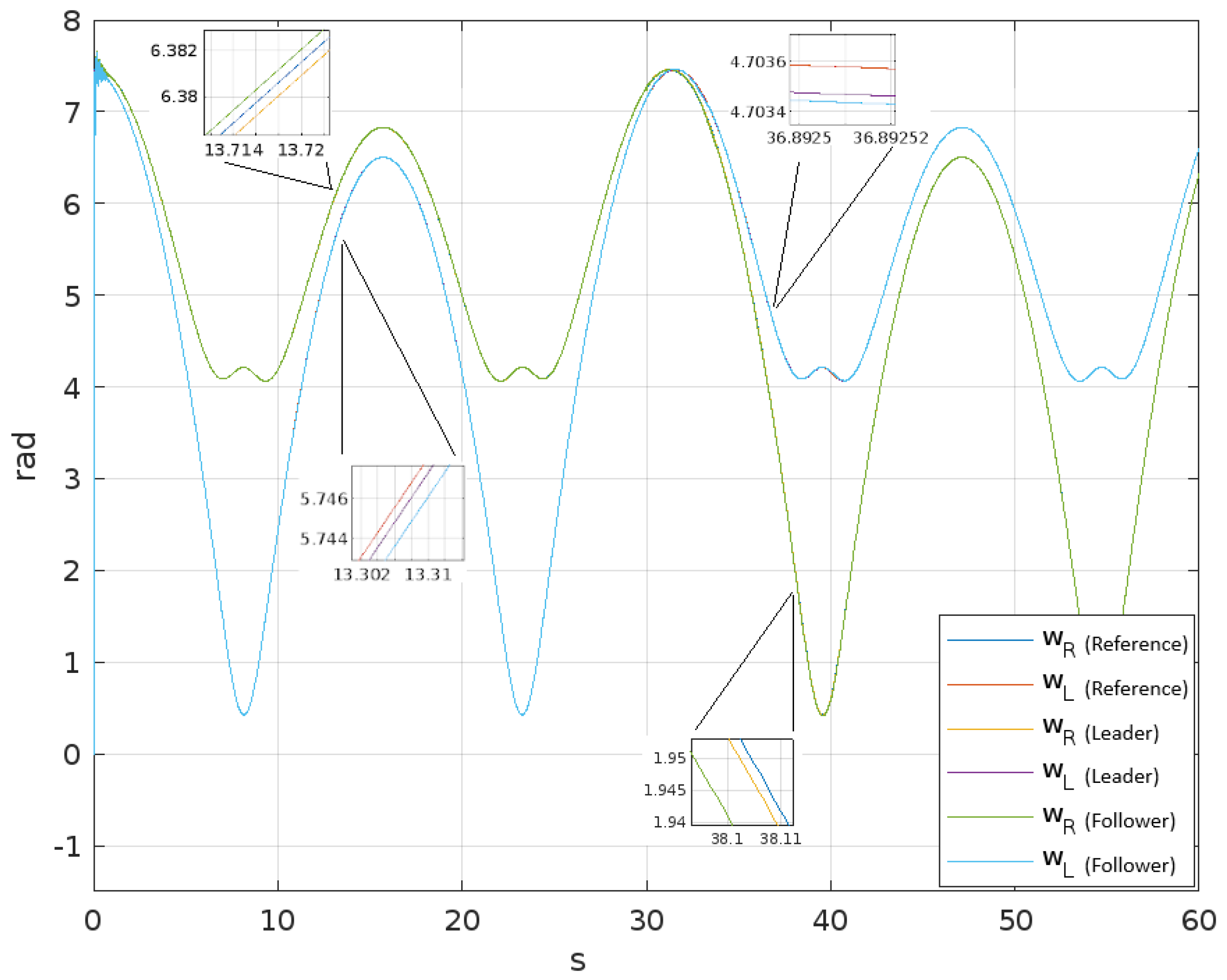
In Figure 3, we can observe the desired velocities w R and w L in blue and red, respectively. Additionally, the velocities w R and w L of the leader are shown in yellow and purple, while those of the follower are represented by green and pale blue. Notice that both agents closely follow the desired velocity with minimal error. However, the error of the follower agent is slightly larger than that of the leader, as it relies on the angular velocities of the leader. It is noteworthy that even during periods of parameter variation and external disturbances, the tracking error remains small, indicating that the controllers effectively mitigate these disturbances.
The functions of significance are those outlined by b ( z ) , as they encapsulate all uncertainties. Figure 4 displays the dynamic estimation of these uncertain functions, b ( z ) , achieved through the proposed estimation method based on the RHONN.
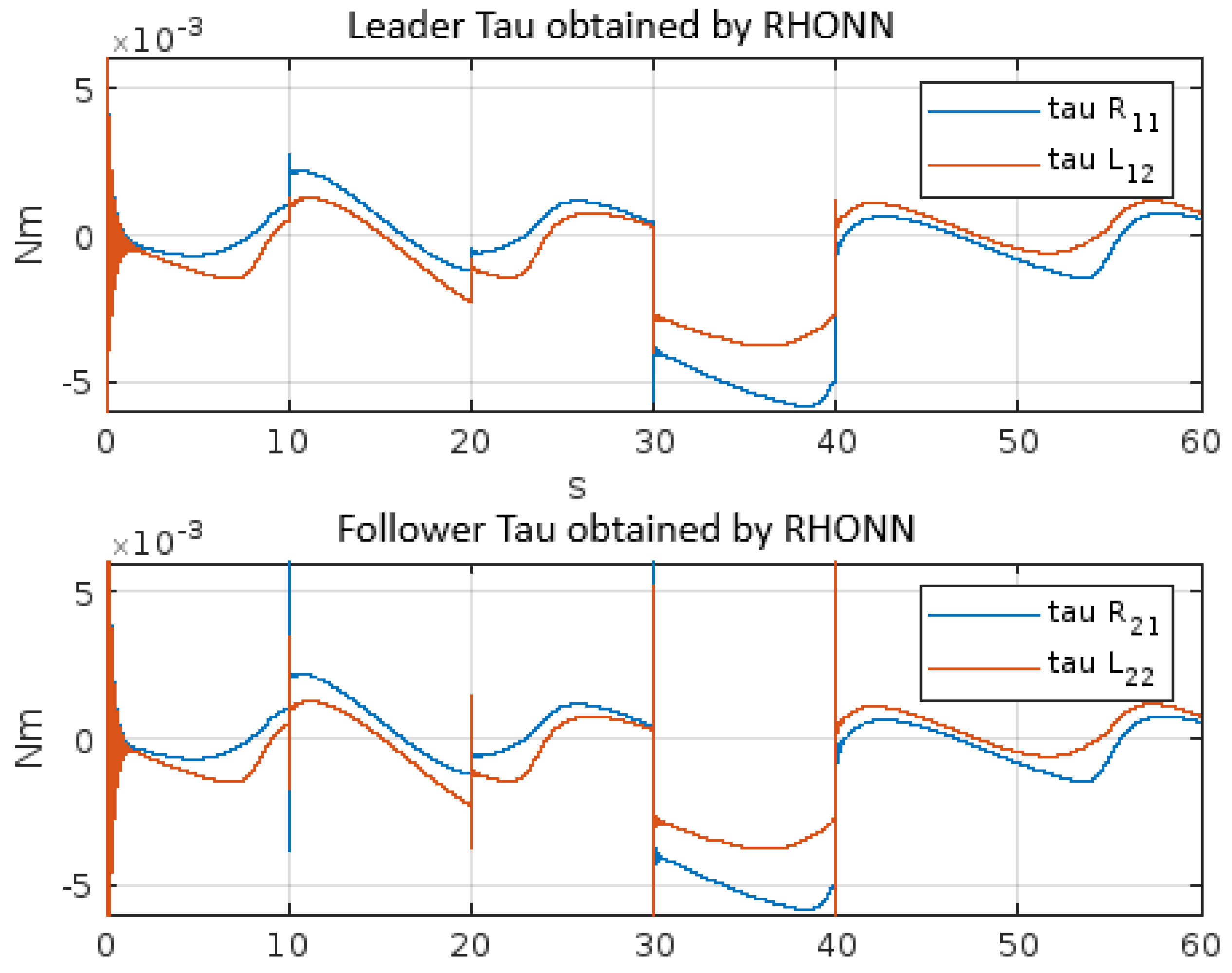
In Figure 5, we present the two set of torques generated by the design controller. During the parameter variation interval, the control action increases as the motors required additional torque because of the mass increase. During the external disturbances period, the torque becomes more negative and exhibits greater amplitude, effectively compensating for the rising velocity.
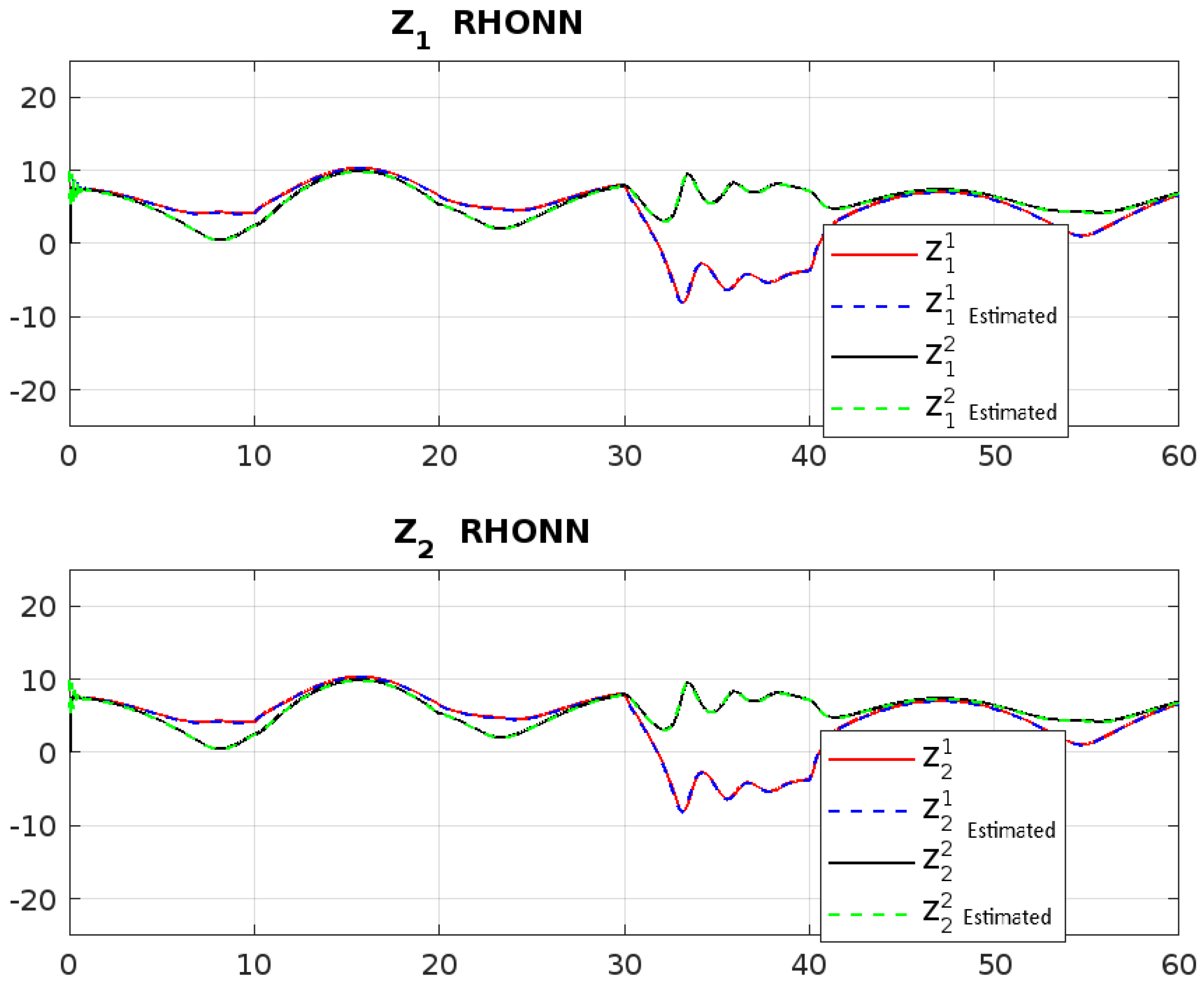
In Figure 6, the states of the transformed system and the estimated corresponding states via the RHONN are presented; these estimated states are used to determine the estimates of the uncertain function b ( z ) .
Figure 7 shows the trajectories in the Cartesian plane. It is noteworthy that the leader and follower start in different positions without running into any collision. Additionally, at 10 s, 20 s, and 40 s, discrepancies and perturbations in the systems are evident, as illustrated in Figure 5. It is important to stress that even in the presence of the disturbances, the mobile robots remain in the reference trajectory. This underscores the capability of the neuro-robust controllers to compensate for such disturbances, keeping the errors between the references and the output systems close to zero. It is crucial to mention that the controllers solely have access to velocity measurements; therefore, the controller is considered robust against external perturbations, parameter variations, and discrepancies of the model.

5. Discussion and Conclusions

In this contribution, a neuro-robust controller designed for controlling leader–follower mobile robots is proposed. This controller operates properly and shows satisfactory behavior in the presence of parameter variations and additional disturbances. Specifically, the leader tracks the reference trajectory while the follower accurately tracks the leader’s path, even in the presence of perturbations and parameter uncertainties. The main advantage of the proposed scheme lies in its ability to eliminate the necessity for complete knowledge of system parameters and the measurement of the entire state. This control consists of two parts: a linearizing controller based on a system diffeomorphic transformation and a neural network parameter estimation. The transformed system is such that the parameters are lumped into a single uncertain nonlinear function; this function is then estimated using an RHONN, eliminating the necessity of estimating each system parameter uncertainties and unmodeled dynamics separately. The estimates derived are integrated into the controller for compensation. Both the estimator and the controller only require measurements of the output and an estimate or nominal value of the parameters. The asymptotic tracking of the reference trajectory is demonstrated utilizing the Lyapunov method. The results are validated via numerical simulation. Furthermore, this same methodology can be applied to diverse systems and extended to trajectory tracking using position measurements, not limited to velocity measurements.

Author Contributions

Conceptualization, G.S.-P., D.R.-C. and M.B.-V.; methodology, G.S.-P., D.R.-C., M.B.-V. and M.A.P.-C.; software, G.S.-P., D.R.-C. and M.B.-V.; validation, G.S.-P. and M.B.-V.; formal analysis, G.S.-P., D.R.-C., M.B.-V. and M.A.P.-C.; investigation, G.S.-P., D.R.-C. and M.B.-V.; resources, G.S.-P., M.B.-V. and M.A.P.-C.; data curation, G.S.-P. and M.B.-V.; writing—original draft preparation, G.S.-P., D.R.-C. and M.B.-V.; writing—review and editing, G.S.-P., D.R.-C., M.B.-V. and M.A.P.-C.; visualization, G.S.-P., D.R.-C. and M.B.-V.; supervision, G.S.-P., D.R.-C. and M.A.P.-C.; project administration, G.S.-P.; funding acquisition, M.A.P.-C. All authors have read and agreed to the published version of the manuscript.

Funding

This research was funded by Universidad de Guadalajara CUCEI.

Institutional Review Board Statement

Not applicable.

Informed Consent Statement

Not applicable.

Data Availability Statement

The simulations data supporting this paper are from previously reported studies, which have been cited. The processed data are available from the corresponding author upon request ([email protected]).

Conflicts of Interest

The authors declare that there are no conflicts of interest regarding the publication of this paper.

References

  1. Loganathan, A.; Ahmad, N.S. A systematic review on recent advances in autonomous mobile robot navigation. Eng. Sci. Technol. Int. J. 2023, 40, 101343. [Google Scholar] [CrossRef]
  2. Alatise, M.B.; Hancke, G.P. A Review on Challenges of Autonomous Mobile Robot and Sensor Fusion Methods. IEEE Access 2020, 8, 39830–39846. [Google Scholar] [CrossRef]
  3. Wang, Y.; Cheng, L.; Hou, Z.; Yu, J.; Tan, M. Optimal formation of multi-robot systems based on recurrent neural network. IEEE Trans. Neuronal Netw. Learn. Syst. 2016, 27, 322–333. [Google Scholar] [CrossRef] [PubMed]
  4. Lian, K.Y.; Hsu, H.; Tsai, T.S. Leader-Follower mobile robots control based on light source detection. IEEE Sens. J. 2019, 19, 11142–11150. [Google Scholar] [CrossRef]
  5. Soorki, M.N.; Talebi, H.A.; Nikravesh, S.K.Y. Robust leader-following formation control of multiple mobile robots using Lyapunov redesign. In Proceedings of the IECON 2011—37th Annual Conference of the IEEE Industrial Electronics Society, Melbourne, VC, Australia, 7–10 November 2011; pp. 277–282. [Google Scholar]
  6. Rabani, M.J.; Memon, A.Y. Trajectory tracking and stabilization of nonholonomic wheeled mobile robot using recursive integral backstepping control. Electronics 2021, 10, 1992. [Google Scholar] [CrossRef]
  7. Hassan, N.; Saleem, A. Neural network-based adaptive controller for trajectory tracking of wheeled mobile robots. IEEE Access 2022, 10, 13582–13597. [Google Scholar] [CrossRef]
  8. Meng, J.; Liu, A.; Yang, Y.; Wu, Z.; Xu, Q. Two-wheeled robot platform based on PID control. In Proceedings of the 5th International Conference on Information Science and Control Engineering (ICISCE), Zhengzhou, China, 20–22 July 2018; pp. 1011–1014. [Google Scholar]
  9. Majid, A.; Mohamed, Z.; Basri, M. Velocity control of a unicycle type of mobile robot using optimal PID controller. J. Teknol. Sci. Eng. 2016, 78, 4–7. [Google Scholar] [CrossRef]
  10. Michel, F.; Sanchez, E.N.; Alanis, A.Y.; López-Franco, C. Neural control for a differential drive wheeled Mobile robot integrating stereo vision feedback. Comp. Sist. 2015, 19, 429–443. [Google Scholar]
  11. Isidori, A. Nonlinear Control System, 3rd ed.; Springer: London, UK, 1995. [Google Scholar]
  12. Femat, R.; Alavarez, J.; Castillo, B.; González, J. On Robust Chaos suprression in class of nondriven oscillators: Application to the Chua’s circuit. IEEE Trans. Circuits Syst. 1999, 46, 1150–1152. [Google Scholar] [CrossRef]
  13. Femat, R.; Solis-Perales, G. Robust Synchronization Via Geometrical Control: A General Framework. Lect. Notes Control Inf. Sci. 2008, 378, 99–137. [Google Scholar]
  14. Rovithakis, G.A.; Christodoulou, M.A. Adaptative Control whit Recurrent High-Order Neural Networks, 1st ed.; Springer: London, UK, 2000. [Google Scholar]
  15. Arana-Daniel, N.; Alanis, A.Y.; Lopez-Franco, C. Neural Networks for Robotics: An Engineering Perspective; CRC Press, Inc.: Boca Raton, FL, USA, 2018. [Google Scholar]
  16. Alanis, A.Y.; Arana-Daniel, N.; Lopez-Franco, C. Artificial Neural Networks for Engineering Applications; Academic Press: Cambridge, MA, USA; Elsevier: Amsterdam, The Netherlands, 2019. [Google Scholar]
  17. Hopfield, J. Neurons with graded response have collective computational properties like those of two-state neurons. Proc. Nat. Acad. Sci. USA 1984, 81, 3088–3092. [Google Scholar] [CrossRef] [PubMed]
  18. Ricalde, L. Inverse Optimal Adaptive Recurrent Neural Control with Constrained. Ph.D. Thesis, Cinvestav, Guadalajara, Mexico, 2005. Available online: https://repositorio.cinvestav.mx/handle/cinvestav/452 (accessed on 1 May 2024).
  19. Alanis, A.Y.; Lopez-Franco, M.; Arana-Daniel, N.; Lopez-Franco, C. Discrete-time neural identifier for electrically driven nonholonomic mobile robots. In Proceedings of the 2011 International Joint Conference on Neural Networks, San Jose, CA, USA, 31 July–5 August 2011; pp. 1067–1073. [Google Scholar]
  20. Jian’an, X.; Mingjun, Z.; Jian, Z. Kinematic model identification of autonomous mobile robot using dynamical recurrent neural networks. In Proceedings of the IEEE International Conference Mechatronics and Automation, Niagara Falls, ON, Canada, 29 July–1 August 2005; Volume 3, pp. 1447–1450. [Google Scholar]
  21. Wang, S.; Shao, X.; Yang, L.; Liu, N. Deep Learning Aided Dynamic Parameter Identification of 6-DOF Robot Manipulators. IEEE Access 2020, 8, 138102–138116. [Google Scholar] [CrossRef]
  22. Nicosia, S.; Tomei, P. State observation of elastic joint robots. IFAC Proc. Vol. 1988, 21, 47–52. [Google Scholar] [CrossRef]
  23. Kim, Y.H.; Lewis, F.L. Neural network output feedback control of robot manipulator. IEEE Trans. Robot. Autom. 1999, 15, 301–309. [Google Scholar] [CrossRef]
  24. Trujillo, D.; Morales, L.A.; Chávez, D.; Pozo, D.F. Trajectory Tracking Control of a Mobile Robot using Neural Networks. Emerg. Sci. J. 2023, 7, 1843–1862. [Google Scholar] [CrossRef]
  25. Kosmatopoulus, E.B.; Polycarpou, M.M.; Christodoulou, M.A.; Ioannou, P.A. High order neural network structures for identification of dynamical systems. IEEE Trans. Neural Netw. 1995, 6, 422–435. [Google Scholar] [CrossRef] [PubMed]
  26. Kosmatopoulus, E.B.; Christodoulou, M.A.; Ioannou, P.A. Dynamical neural networks that ensure exponential identification error convergence. Neural Netw. 1997, 10, 299–314. [Google Scholar] [CrossRef] [PubMed]
  27. Dhaouadi, R.; Hatab, A. Dynamic modelling of differential-drive mobile robots using lagrange and Newton-Euler methodologies: A unified framework. Adv. Robot. Automat. 2013, 2, 107. [Google Scholar]
  28. Khalil, H.K. Nonlinear Systems; Prentice Hall: Upper Saddle River, NJ, USA, 2002. [Google Scholar]
  29. Vinod, R.N.; Mathew, T.A. Design, Simulation and implementation of cascaded path tracking controller for a differential drive mobile robot. In Proceedings of the 2015 International Conference on Advances in Computing, Communications and Informatics (ICACCI), Kochi, India, 10–13 August 2015; pp. 1085–1090. [Google Scholar]
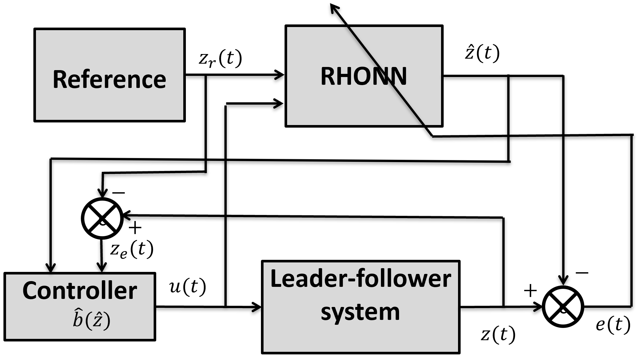
Figure 1. Control scheme.
Applsci 14 05374 g001
Figure 2. Differential mobile robot model [27].
Applsci 14 05374 g002
Figure 3. Time evolution of the angular velocities. Zoomed-in sections illustrate the small differences between references and the outputs velocities, even in the presence of the disturbances.
Applsci 14 05374 g003
Figure 4. Dynamic estimation of the uncertain functions b using an RHONN. All the unknown system parameters are estimated online; note that there is a small transient period due to the disturbances.
Applsci 14 05374 g004
Figure 5. Neuro-robust control signals (torques), where one can see the changes in the control value required to compensate the disturbances at t = 10 s, 20 s, 30 s, and 40 s.
Applsci 14 05374 g005
Figure 6. Dynamic evolution of the transformed states and their estimations are shown. Solid lines depict the output system and its derivative, while dashed lines illustrate the estimates of the transformed states via the RHONN.
Applsci 14 05374 g006
Figure 7. Trajectories in the Cartesian plane, where the leader and follower have different initial conditions. Points marked as ∗ where the perturbations and variation of the parameters are applied.
Applsci 14 05374 g007
Table 1. Parametric values for simulation 1 [29].
ParameterValue
NominalVariation
M 2.2 kg 4.4 kg
d 0.04 m 0.04 m
R 0.03 m 0.03 m
L 0.0975 m 0.0975 m
J 4.1 × 10 6 kg-m 4.1 × 10 6 kg-m
m 1 0.01720.0344
m 2 0.0158 0.0316
V 5.2071 × 10 4 0.0010
Disclaimer/Publisher’s Note: The statements, opinions and data contained in all publications are solely those of the individual author(s) and contributor(s) and not of MDPI and/or the editor(s). MDPI and/or the editor(s) disclaim responsibility for any injury to people or property resulting from any ideas, methods, instructions or products referred to in the content.