Modelling of the Luminance Coefficient in the Light Scattered by a Mineral Mixture Using Machine Learning Techniques

Abstract

The primary objective of the research and analysis reported in this article was to determine an effective method for predicting the luminance coefficient of the mineral mixture for asphalt concrete and stone mastic asphalt. The luminance of the mineral mixture determines the final luminance value of the surface. Predicting the luminance coefficient quickly will significantly improve the mineral–asphalt mix design efficiency in selecting aggregates that meet functional requirements and increase the brightness of the surface. The research process consisted of two stages. The first stage covered modelling the Qd luminance coefficient of aggregate, taking into account its petrographic analysis. The second fundamental stage, based on the research of the first stage, concerned the modelling of the luminance coefficient of the mineral mixture, taking into account the percentage share of a given component, its grain size, and its photometric properties. An effective technique of reinforced trees was used for modelling. As a result of its application, a model match to experimental data was achieved at the level of 87%. It has also been shown that the greatest impact on increasing the luminance coefficient of the mineral mixture was the use of light aggregate (quartzite sandstone or limestone) with a grain size of 2/5 in quantities > 40% or 8/11 in quantities > 60%. Furthermore, the quartzite sandstone aggregates with a grain size of 5/8 had the highest efficiency in lightening the mineral mixture. However, the use of basalt aggregates of the same fraction significantly worsened the photometric properties of the mineral mixture. An important element of the research was also to indicate that the mineralogical composition of the aggregate is crucial for an accurate assessment of its luminance coefficient.

1. Introduction

According to the nomenclature used in European countries, light surfaces are those in which light aggregates and synthetic binders have been used, either colourless or in light colours, caused by the presence of the appropriate pigment. On the other hand, brightened surfaces are those in which traditional asphalts have been used as binders, while the aggregates are from the light group. Bright surfaces are defined as surfaces whose wear layer visually gives the impression of a bright surface. Invariably, in these types of solutions, the aggregate itself [1] is an important element. The International Commission on Illumination (CIE) [2] introduced the concept of luminance in 1982 to evaluate the brightness of surfaces. As a result of this decision, many methods of assessing this parameter have emerged. The purpose of illuminating roads, evaluated by luminance coefficients q, was the need to improve the visibility of objects and traffic participants on the road while minimising driver discomfort. The assessment of road surface luminance is complex and still requires the refinement of measurement methods [3]. CIE introduced the R class system, according to which, each surface is classified into one of four classes from R1 to R4. Each of the four classes has a defined light reflection array (r-table) containing a reduced luminance coefficient [4]. Unfortunately, the R classification is based on measurements from the 1960s and 1970s, and it should be taken into account that there have been changes in the technology of making asphalt surfaces (mma) and the requirements for macrotexture, and new types of asphalt aggregates [5] have been introduced.

A fundamental fact, increasingly noticeable in scientific publications and industry articles, is that bright surfaces heat up less during periods of intense sunlight and provide a higher contrast of the road profile compared to the roadside. It should not be forgotten that a very important element of road illumination is also the reduction of the amount of energy required to ensure adequate visibility at night. In this aspect, the amount of energy consumed by lighting is about 1.3% used by road lighting in the EU [6]. However, the following question remains: what should be considered when lightening the surface? The reflection of a light beam from the surface of the road is a function of the physical state of the road and its nature, as well as the direction of the light beam and observation conditions [5]. Different surfaces may have different reflection characteristics, even though the light intensity (measured in lux) is the same. Along with the change in reflective properties of road surfaces, the luminance of pavement will also change [7]. Luminance is closely related to the type of aggregate and the state of surface wear. Reflection from the road surface is a function of the physical condition of the road and its character, as well as from the direction of its illumination and observation conditions [5]. Different surfaces can have various reflection characteristics, which depend on the texture of the surface and its age, the materials making up the surface, the binding materials, and the ways of arrangement. The criterion for their acceptance still remains its operational features [8]. Some light-coloured aggregates, such as quartzite sandstone, are aggregates obtained from rocks with acidic reactions with an elevated level of SiO₂. They have high roughness coefficients that improve the anti-slip properties of the road surface [1,9]. On the other hand, limestone aggregates, also of a light colour, are characterised by excellent adhesion to aggregates but have low roughness. Therefore, there are certain contradictions between the luminance of the aggregate and its potential for use. Despite the awareness of technologists that the type of material in the road surface affects the luminance of the surface, the phenomenon of light reflection is not directly taken into account when designing a mixture in work [10]. This is mainly because there are no studies that would allow even approximate surface luminance value to be obtained based solely on data about the components of the mineral (mm) or mineral–asphalt (mma) mixture.

In the European Union, road lighting design is subject to regulations, with some deviations depending on the member country. For the region of Poland, the document [11] applies, which dictates the way lighting design takes into account the luminance coefficient Qo. The average luminance coefficient determines the weighted average of luminance coefficients for a certain area, in which the weights are the corresponding solid angle observation values. The average luminance factor, Qo, can be calculated or read from the r-table using the weighting factor procedure [12]. It has been demonstrated that the average luminance coefficient Qo is strongly correlated with the average luminance produced on the road surface [5]. In the 1990s, an alternative to Qo was introduced in the form of the luminance coefficient under diffuse lighting Qd. The alternative “brightness” parameter Qd, i.e., the luminance coefficient under diffuse illumination has been adopted for road marking; however, the Qo parameter is still used in the road surface classification system adopted for road lighting. The ability to accurately bring down the Qo values using r-tables to the Qd measure, which was to some extent included in the CIE document [13], is significant. The use of the Qd coefficient is possible due to the occurrence of a large correlation of the Qo coefficient with the average luminance generated on the road surface [5].

Unfortunately, there are still no mathematical models to effectively predict the luminance coefficient of the aggregate/asphalt mixture under diffuse illumination Qd. The existence of such a model or method of determination would allow the photometric properties of aggregates to be considered in the design of an asphalt mix. The Qin article [14] uses a linear regression model in the form of multiple regression to calculate perceived luminance in the tunnel interior lighting environment. It was pointed out that this type of regression technique is only applicable to the object under study, and its generalisation requires consideration of more factors. A reason for the low applicability of regression models based on the least squares method may be the observations in the work of Mazurek et al. [15]. It indicates that the probability distribution of the luminance ratio is not normal. The fact that certain minerals are present means that the probability density function is not symmetrical and thus precludes the wider use of techniques based on parametric testing. Therefore, the data mining (DM) technique should be proposed as an effective method. This method provides simple regression or classification rules. However, it requires a large learning dataset as the error rate is not as controllable as it is when using experiment planning techniques [16]. In addition, it also requires a full validation of the adopted model to be performed. Solutions to complex problems for which no mathematical model is known a priori are quite rare in road engineering using data mining techniques. Much more commonly, data mining techniques are so far mainly used to correctly predict the mechanical or physical properties of road materials. In the work of Rebelo et al. [17], a number of DM techniques were used to effectively predict the water resistance of mineral–asphalt mixtures. Gong et al. used DM to improve the rutting resistance of pavements [18]. In contrast, Guo and Hao’s work [19] used a random forest algorithm to assess pavement durability, using information on emerging damage. At the recent EATA 2023 conference in Gdańsk (Poland), many works were presented in which machine learning techniques were used to identify dangerous road conditions. The work of Phan et al. [20] uses machine learning techniques (convolutional neural networks) to identify hazardous road surface conditions. Also, the estimation of the stiffness modulus was determined successfully using the FWD apparatus, taking into account a number of factors related to the measurement by means of artificial neural network (ANN) or support vector machine (SVM) techniques [21,22]. The undoubted advantage of data mining (DM) methods is the consideration of a number of variables, both qualitative and quantitative. It can therefore be used to predict road performance parameters such as IRI [23] or skid resistance (SVR) [24].

There was much less interest in DM techniques for predicting the luminance coefficient of asphalt pavements and the aggregate itself. It should be noted that the evaluation of these parameters is complex and depends on the aggregate system, its origin, the macrotexture of the pavement, etc. The degree of complexity in the prediction of the luminance ratio means that classical methods based on the least squares method will be neither efficient nor effective. There are few studies that attempt to apply DM techniques to the assessment of luminance ratio. In their work, A. Del Corte-Valiente et al. used DM techniques to manage street lighting [25]. In addition, the use of machine learning techniques is being used successfully to assess luminance phenomena in public buildings [26,27].

Despite advanced luminance ratio measurement methods, there are insufficient analyses of the extent of aggregate luminance ratio estimation in the world literature. The conclusions of the study, as reported in [15], indicate that the mineralogical composition of the aggregate is an important aspect in assessing the luminance level of the aggregate. The promising results have encouraged further work to evaluate the luminance coefficient of the mineral mix. The ability to develop an effective DM model for a mineral mix will allow the luminance ratio of a mineral–asphalt mix to be effectively predicted with only information on the luminance of its components. Therefore, the stated aim of the research was to determine the rules and relationships among mineralogy, aggregate grain size, the percentage of components, and the luminance of the mineral mixture using machine learning techniques.

2. Materials and Methods

2.1. Aggregate

Aggregate meeting the Polish requirements of WT-1/2014 [28] and PN-EN 13043 [29] for the construction of wearing layers of asphalt pavements was used in this study. Aggregates were taken using the quartering method. Aggregates for this study were selected using the quartering method. This is a collection of aggregates that are commonly available and used for pavement construction layers that came from areas of southern Poland. The petrographic identification, granulation, and origin of the aggregate are shown in

Table 1. Aggregate collection used to make mineral mixtures.

No.	Type of Aggregate	Granulation	Type	Region
1.	Amphibolite	0/2, 5/8, 8/11	metamorphic	Lower Silesia
2.	Basalt	2/5, 5/8, 8/11, 16/22	igneous	Lower Silesia
3.	Gabro	2/5, 5/8, 8/11	igneous	Lower Silesia
4.	Granite	2/8, 8/16, 16/22	igneous	Lower Silesia
5.	Quartzite Sandstone (Quartzite) 1	0/2, 2/5, 5/8, 8/11, 8/16	sedimentary	Holy Cross Mountains
6.	Palobasalt (Melaphyre) 2	0/2, 2/5, 5/8, 8/11, 8/16	igneous	Lower Silesia
7.	Limestone	0/2, 2/8, 4/11, 5/11, 5/8, 8/11, 8/16, 16/22	sedimentary	Holy Cross Mountains

¹ In figures denoted as quartzite to maintain consistency with [15]; ² in figures denoted as melaphyre to maintain consistency with [15].

.

Table 1 also provides information on selected physical parameters of the aggregate that is intended for wearing courses. All aggregate types met the requirements of EN 13043 [30] specifying the properties of aggregates for use in bituminous mixtures. Selected characteristics are shown in

Table 2. Performance of aggregate set used to create a DM model.

No.	Type of Aggregate	Grain Size	LA [31]	PSV [32]	ρa [33]	Methylene Blue Test [34]	Grading of Filler Aggregates [35]	Flakiness Index [36]
1.	Amphibolite	0/2, 5/8, 8/11	<25	>56	2.84	5÷7 *	max. 16 */max. 2 **	max. 20 **
2.	Basalt	2/5, 5/8, 8/11, 16/22	<10	>50	2.96		max. 1 **	max. 18 **
3.	Gabro	2/5, 5/8, 8/11	<15	>50	2.63 ÷ 3.0		max. 1 **	max. 15 **
4.	Granite	2/8, 8/16, 16/22	<15	>50	2.65		max. 1 **	max. 15 **
5.	Quartzite Quartzite	0/2, 2/5, 5/8, 8/11, 8/16	<25	>56	2.64		max. 14 */max. 1 **	max. 14 **
6.	Melaphyre	0/2, 2/5, 5/8, 8/11, 8/16	<15	>56	2.75		max. 14 */max. 1 **	max. 18 **
7.	Limestone	0/2, 2/8, 4/11, 5/11, 5/8, 8/11, 8/16, 16/22	25 ÷ 30	44 ÷ 56	2.69 ÷ 2.72	-	max. 16 */max. 2 **	max. 17 **

*—For fine crushed aggregate (D ≤ 2 mm), **—for coarse crushed aggregate (D > 2 mm).

.

It was essential to collect the representative sample correctly. Aggregate samples were taken from an aggregate stockpile at five locations. The laboratory sample for testing was obtained using the quartering method following EN 933-1 [35]. Limestones (white colour) had a high LA coefficient, which would limit their use for wearing courses. Quartzite is also a white-coloured aggregate. Its LA value was lower than that of the limestone aggregate.

On the other hand, this aggregate obtained the highest PSV value, which suggests its high resistance to polishing and, hence, a decrease in vehicle stopping distance. However, the quartzite aggregate has a low affinity with asphalt, which is a significant limitation when used in asphalt mixes. The guiding idea is to use an aggregate with a maximum PSV, minimum LA, and high adhesion to asphalt. None of the aggregates meet this criterion. Therefore, it is advisable to mix them, but there is a risk that many dark-coloured grains will be found in the mix composition, effectively reducing the mineral mix luminance.

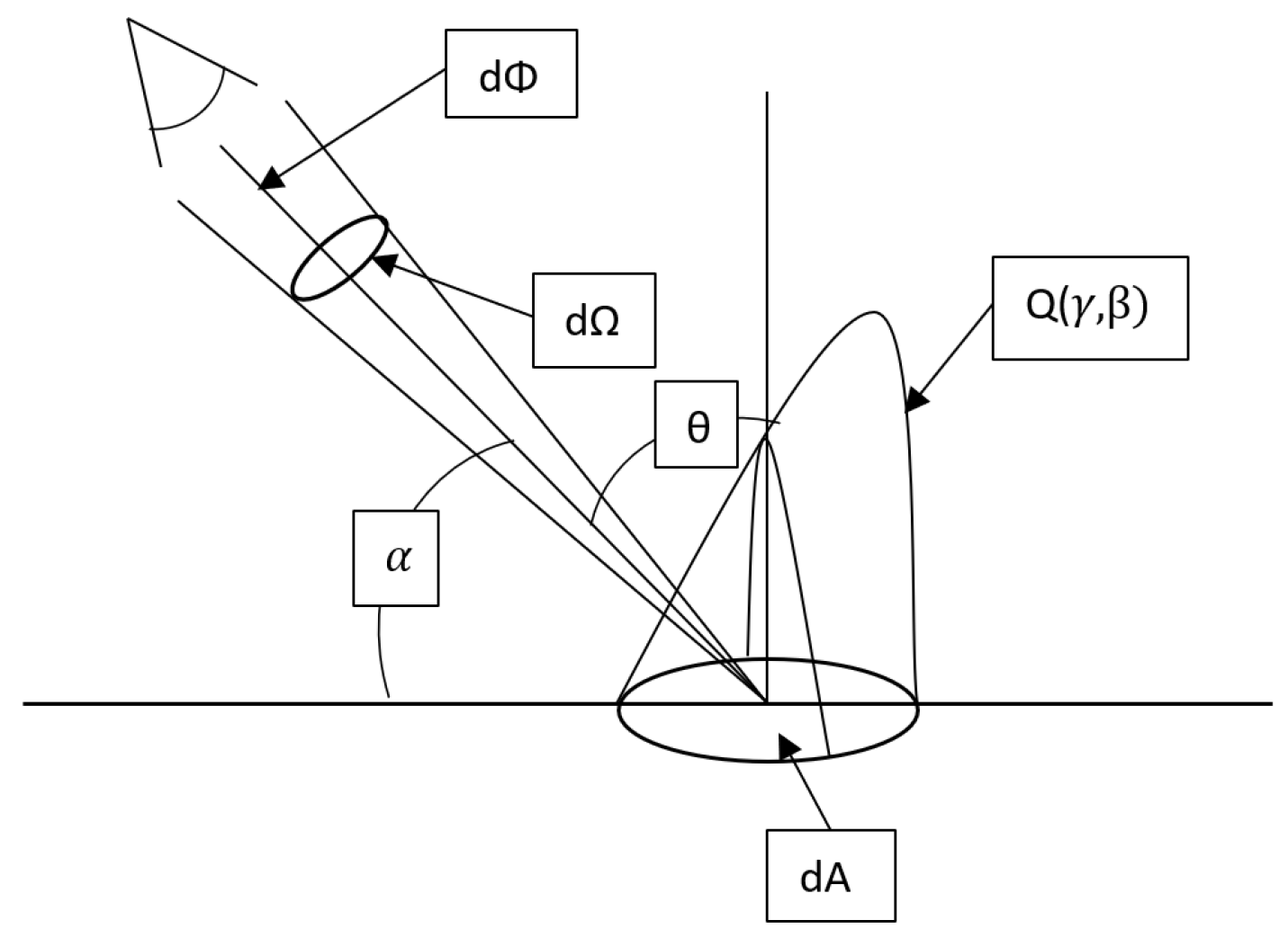
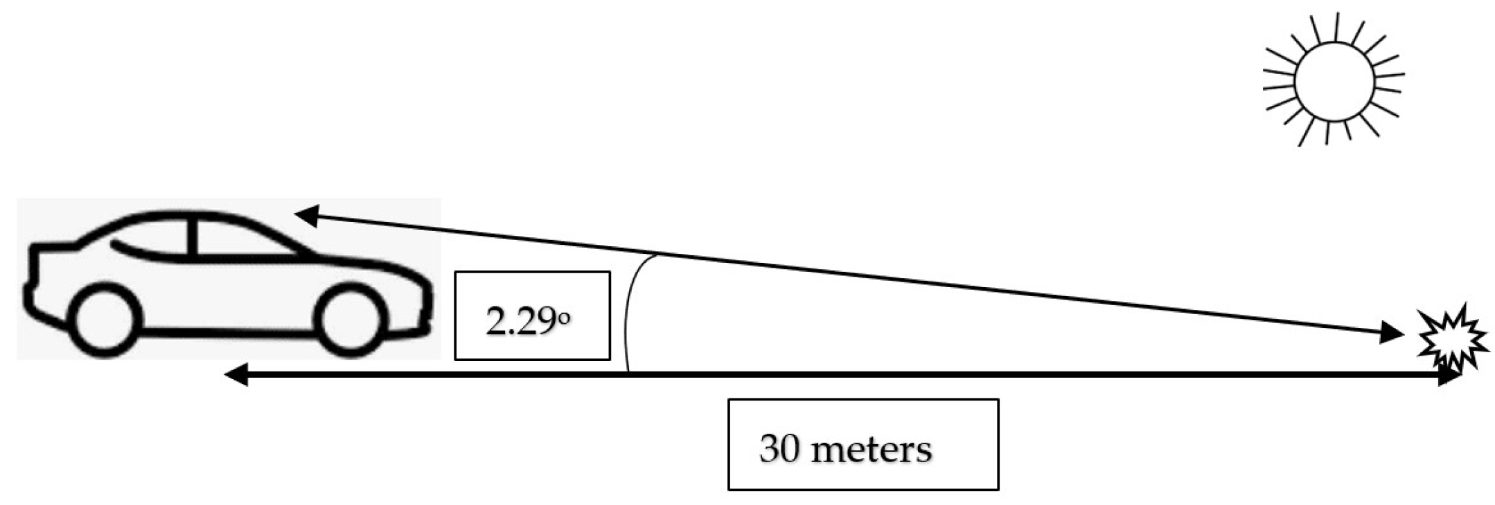
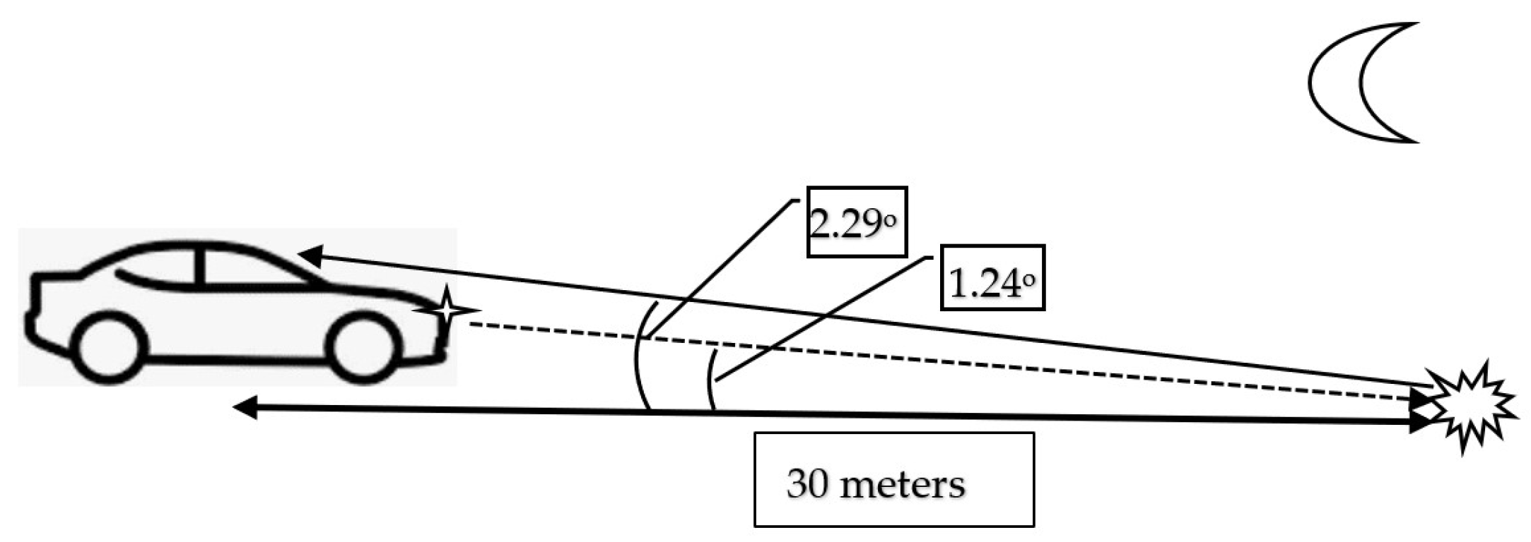
2.2. Luminance Ratio

Road brightness and visibility under artificial light in Europe are related to the distribution of luminance and illumination on the road surface. The intensity of illumination on a road surface refers only to the amount of light reaching the surface, which does not indicate how bright the surface is. Illuminance (E) is the amount of incident light (luminous flux Φ) per unit area (A). The SI unit of illuminance is lux (lx). According to the SI system, illumination is expressed by Formula (1), as follows:

$$\mathrm{E}=\frac{\mathrm{d}\mathsf{\Phi }}{\mathrm{d}\mathrm{A}}$$

(1)

Luminance, on the other hand, is defined as the luminance flux per unit projected area and is a function of the illuminance on the road and the reflectance characteristics of the road surface [37], according to Formula (2), as follows:

$$\mathrm{L}=\frac{\mathrm{d}\mathsf{\Phi }}{\mathrm{d}\mathsf{\Omega }·\mathrm{d}\mathrm{A}·\mathrm{c}\mathrm{o}\mathrm{s}\mathsf{\theta }}$$

(2)

where Φ is the luminance flux, A is the surface, Ω is the spatial noun, and θ denotes the angle between the direction of the solid angle Ω and the emitting normal or reflecting surface A. The geometry required to determine the luminance ratio is shown in Figure 1.

In summary, the reflectance of a surface field can be described by a luminance factor q, which is defined as the luminance of the surface field L, produced by illumination and reflection, divided by the illuminance of the surface plane of the field E according to Formula (3), as follows:

$$\mathrm{q}=\frac{\mathrm{L}}{\mathrm{E}}$$

(3)

The luminance factor q is measured in mcd⋅m⁻²⋅lx⁻¹.

2.3. Diffuse Luminance Coefficient Qd and Surface Reflectance Coefficient RL

EN 1436 [39] defines Qd as the ratio of the luminance of a surface area under diffuse illumination in proportion to the illuminance at the surface plane. Qd is measured using the spectral distribution of illumination according to a standard illuminator representing daylight and an observation angle of 2.29° representing a geometry (observation distance) of 30 m. A representation of the measurement of Qd is represented by the diagram below (Figure 2).

Surface reflection is strong in situations corresponding to driving against the sun. The usual bounce is strong in situations corresponding to riding with the sun back. Suitable light for a standard road configuration when confronted with dry and wet surface conditions is assessed by optimising the lighting distribution function [40]. The degree of reflectivity of a road surface traditionally depends on the averaged luminance coefficient Qo [12] and the mirrored reflectivity S1 [41]. The average luminance expressed by the luminance factor Qo, although still used, is a parameter that is difficult to measure in the small space of a portable instrument. Therefore, from the 1990s onwards, the Qd factor was introduced to characterise the reflectivity of road markings in daylight or under road lighting. Portable units are available and are used widely for road markings and can also be applied to road surfaces. However, no portable instrument determines the precise mirroring coefficient. The luminance factor Qd, used in this study, takes into account the mirror effect, but to a lesser extent than Qo. Therefore, the Qd parameter can be regarded as a reasonable approximation of the Qo value for determining the illuminance required for road lighting design. The Qd factor is also relevant when daylighting is poor (e.g., twilight) [40].

The standardised luminance coefficient Qd for the pavement, associated with the r-table, can be determined using laboratory methods from a cut sample of the pavement under field conditions using a reflectometer or by modern digital image analysis techniques [42]. It is worth mentioning that the maximum luminance that can be obtained for a given area when the surroundings have a constant luminance L is 318 mcd⋅m⁻²⋅lx⁻¹. In contrast, a value of approximately Qd = 52 mcd⋅m⁻²⋅lx⁻¹ is attributed to “black” pavements [41]. This type of luminance factor determines daytime visibility.

Another measure of luminance is the surface reflectance RL (mcd⋅m⁻²⋅lx⁻¹). It is defined as the quotient of the luminance L of the marking surface in the direction of observation by the illuminance E in a plane perpendicular to the direction of incident light and to the area of that reflective surface. The definition of RL is very similar to that of the luminance ratio Qd and has the same unit. Typically, the surface reflectance coefficient RL determines the reflectivity of pavement or horizontal markings illuminated by the light of vehicle lamps. It is also referred to as night visibility. It is important in the absence of road lighting. A diagram of its designation is shown in Figure 3.

Road surfaces generally have RL values in the range of 10 to 30 mcd⋅m⁻²⋅lx⁻¹. In comparison, surfaces intended for road marking (containing glass spheres) can usually achieve at least RL = 150 mcd⋅m⁻²⋅lx⁻¹.

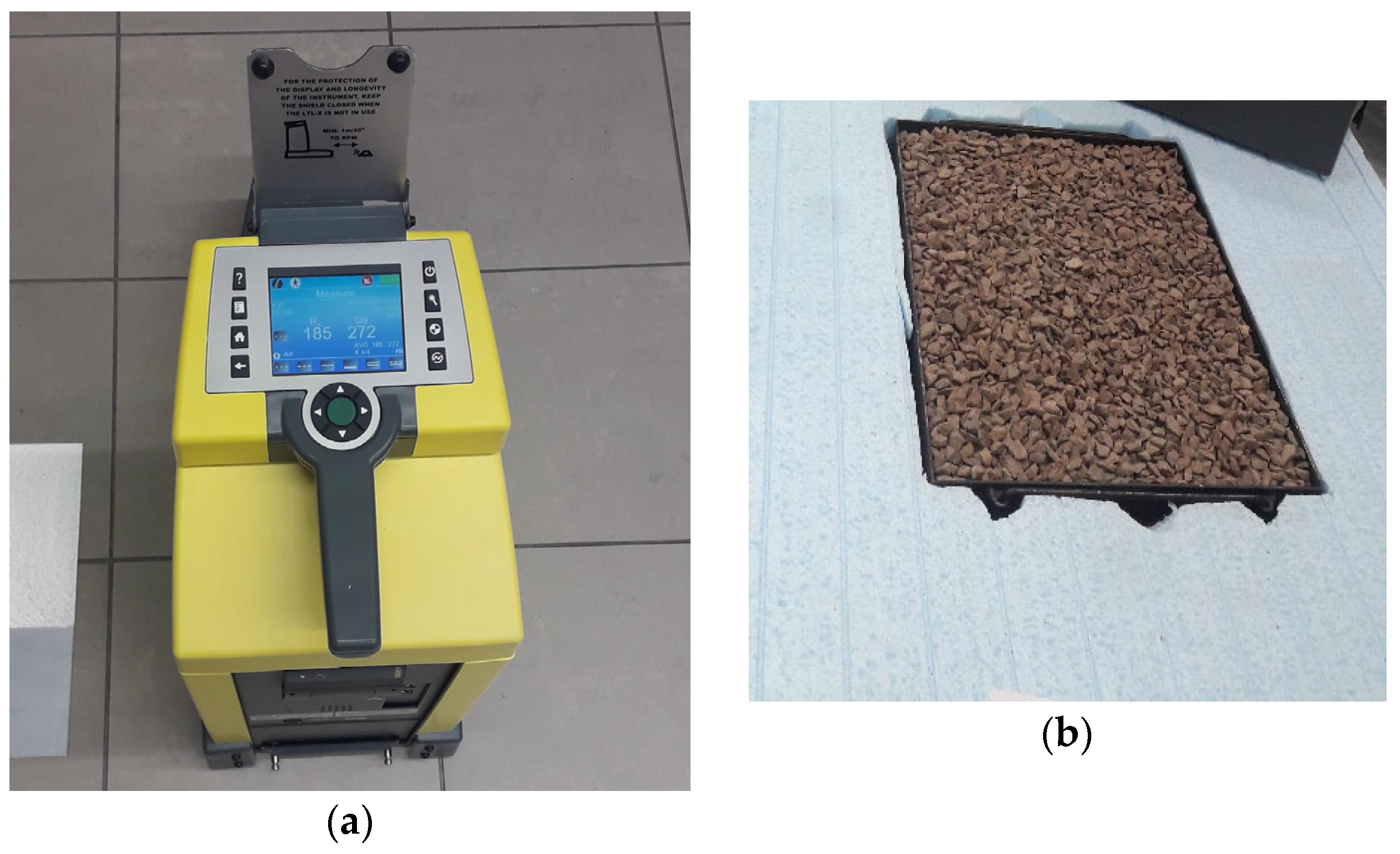
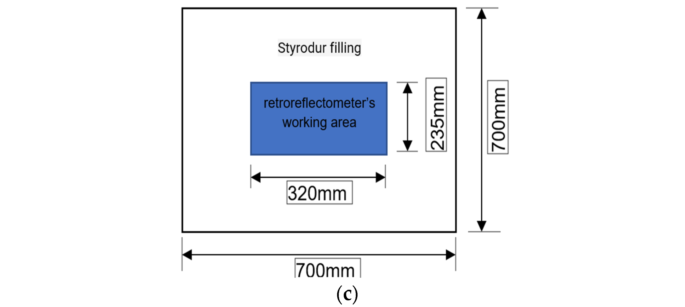
2.4. Test Stand for Measuring the Luminance Ratio

The test form used to test the aggregate and mineral mixtures complied with the orders of WT-2/2014 [43], according to which the stable test area should be 700 mm × 700 mm. In contrast, the void that is not to be measured should be filled with any rigid material. The working area containing the aggregate was sized to match the working area of the retroreflectometer (LTL-X Mark II) and was 320 mm × 235 mm. Each aggregate sample was tested 5 times at different locations in the working area. Another sample was then taken from another location in the aggregate stockpile (series). Each aggregate was assessed using five series. As a result, for the determination of the coefficient, Qd and RL were measured 25 times for each aggregate against each grain size. Each test sample was pre-compacted and levelled with a screed to obtain reference measurement conditions. The test stand is shown in Figure 4.

The test stand was set up to determine the luminance coefficient of aggregates and mineral mixtures. According to the Polish regulations contained in WT-2 [43] and PN-EN 1436 [39], the measurement of the luminance ratio should be carried out at an angle of 2.29° (equivalent to observing the road from a distance of 30 m from the position of a passenger car driver). The measurement field should be a rectangle measuring 185 mm × 50 mm, with an angular spread of ±0.17°. This requirement was met by the LTL-X Mark II device used to perform this study. The device allows two parameters to be specified, Qd and RL, with the possibility of importing the results into a database. The test is performed in fixed diffused light. The sample should be illuminated with a D65 standard light source of constant luminance. The measurement is carried out when the ambient temperature is between 0 and 30 °C and the temperature of the test sample/surface is between 5 and 40 °C. The Portable LTL-X Mark II device does not allow for the use of an observation angle of 1°, which prevents the observation of a section longer than 30 m. Therefore, the value of the scattered light luminance coefficient Qd is an approximation of the luminance coefficient Qo.

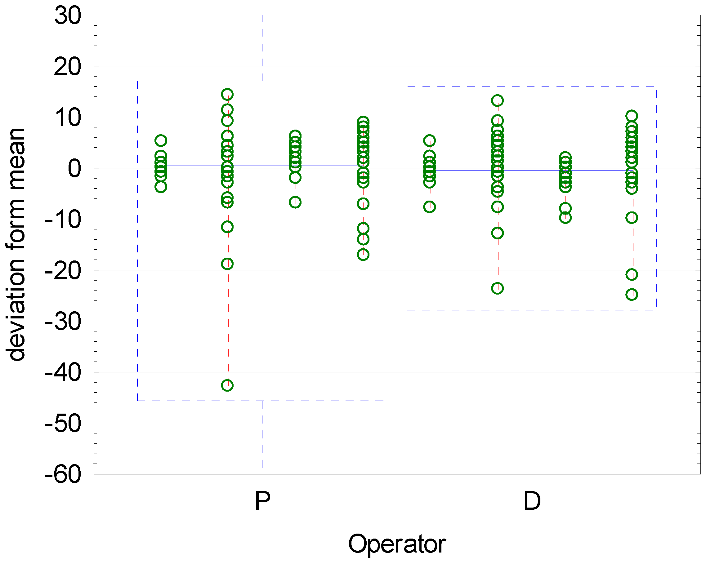
2.5. Validation of the Method

Every research method is subject to measurement error. The source of error may be an operator, the measurement method itself, or inaccuracies resulting from the calibration of the sensors on the measuring device. The effectiveness of the measurement method was assessed to make sure that it is reliable and representative. The method (Section 2.4) involved preparing an original test stand including the preparation of samples. Provisions of ISO 5725-2 [44] were the basis for determining the accuracy and precision of the method. The stability of the measurement process was evaluated using the procedures of the R&R per AIAG [45] based on the analysis of variance (repeatability and reproducibility). To validate the measurement method effectively, the experiment needed careful planning. This involved breaking down the process into specific steps and identifying any factors that might cause variability in the Qd and RL measurements. Hence, the validation process had the following:

• Two operators;
• Two reflectometers;
• Four randomly selected aggregate samples (light and dark).

The results of the method validation are shown in Figure 5.

Two hundred measurements were used in this study. Figure 5 shows the operator codes. Operator P represents measurements conducted at the Kielce University of Technology. Operator D was assigned to another research centre participating in the comparative study. The measurements were performed using a basic group of the following four aggregates: melaphyre 2/5, quartzite 5/8, basalt 8/11, and dolomite 2/8, repeating each measurement four times. As shown in Figure 5, the reproducibility is high, and the repeatability of the results is very similar. However, to definitively determine the process stability, a table summarising the characteristics of the research process is presented below (

Table 3. Assessment of measurement method stability.

Source	Qd		RL
	Value mcd⋅m−2⋅lx−1	% of R&R	Value mcd⋅m−2⋅lx−1	% of R&R
Repeatability	6.41	8.26	2.24	4.45
Reproducibility	0.12	0.01	0.6	0.32
Part	21.37	91.74	10.35	95.23
Total R&R	6.41	8.26	2.32	4.77
Total	22.31	100	10.61	100

).

Repeatability, reproducibility, and the contribution of R&R variability to overall process variability (stability) are crucial characteristics of the measurement method. Table 3 reveals excellent repeatability for both Qd (6.4 mcd⋅m⁻²⋅lx⁻¹) and RL (2.24 mcd⋅m⁻²⋅lx⁻¹ i 0.6 mcd⋅m⁻²⋅lx⁻¹) characteristics. The reproducibility of Qd is 0.1 mcd⋅m⁻²⋅lx⁻¹. These values are quite low, considering the significant variation in aggregate petrography and grain size. The key metric is total R&R, reflecting overall measurement method stability. Qd and RL achieved total R&R values of 8.26% and 4.77%, respectively. According to AIAG procedures, a measurement process with a total R&R below 10% is considered stable. This signifies that the proposed method and its results are representative and highly reproducible by other trained operators using calibrated equipment. Low variability demonstrates the reliability of the measurement method and the resulting data. This stability is a crucial step for building reliable machine learning models. With this confirmation for individual aggregates, this study progressed to analysing mineral mixtures.

2.6. Mineral Mix Grading Curves

The structure of the input mineral mixture set was based on the use of the designed compositions of 30 mineral mixtures intended for actual road surfaces subjected to category KR5-7 (7.3·10⁶ ÷ 52·10⁶ ESAL) traffic loads. The compositions were determined using the limit curves method for asphalt concrete mixtures intended for the wearing course. The aggregate grading curves are summarised below (Figure 6).

The selected mixtures included SMA and AC. The maximum grain size D imposed by WT-2/2014 [43] is 11.2 mm for wearing course mixtures. The top sieve sizes used in the analysis were 8 and 11.2 mm, respectively. The mineral mixture skeleton reflected the maximum variation in aggregate colour. It was important to prepare the mineral mixtures exclusively from the aggregate base given in Table 1.

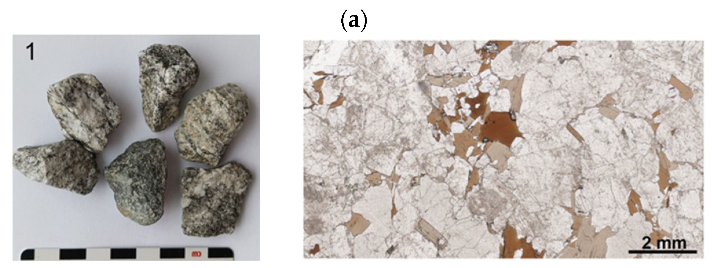
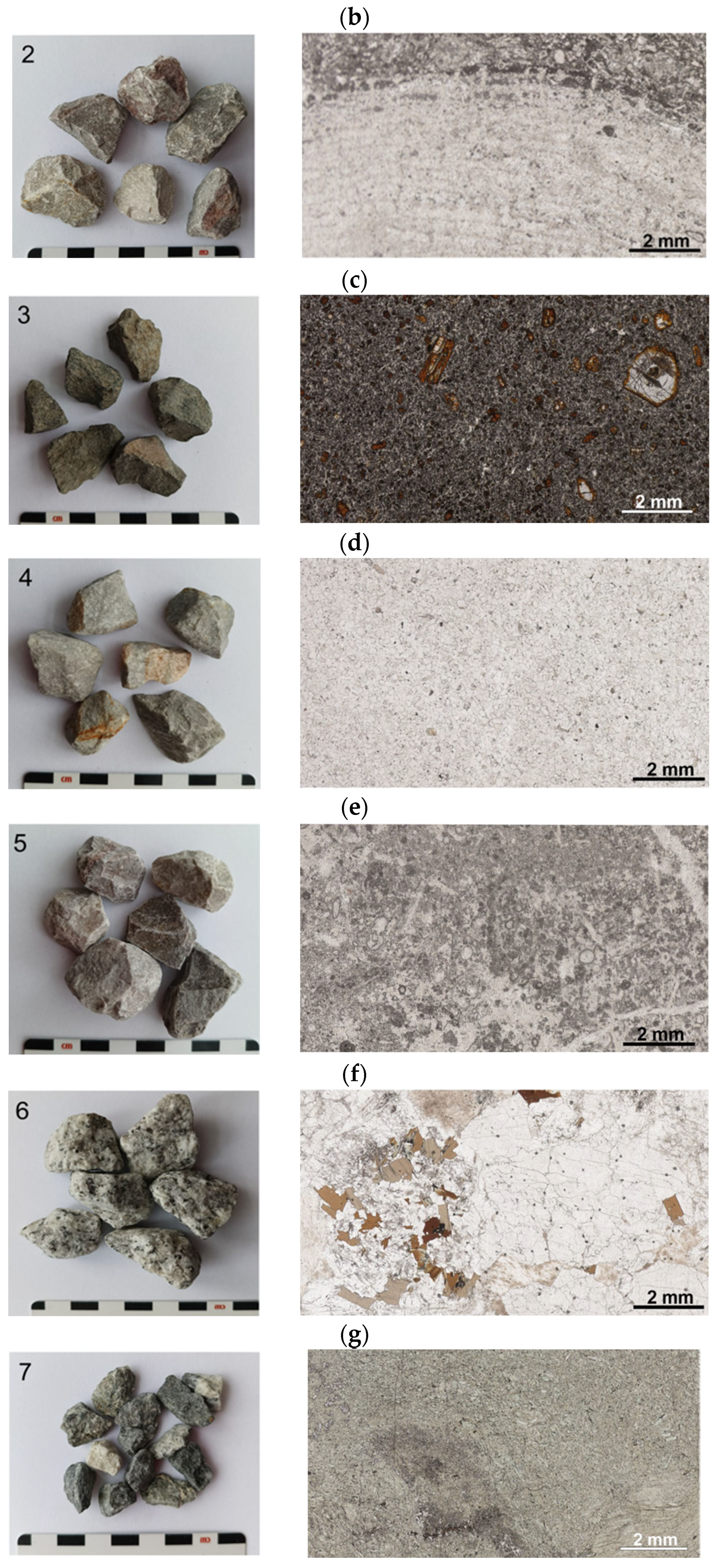
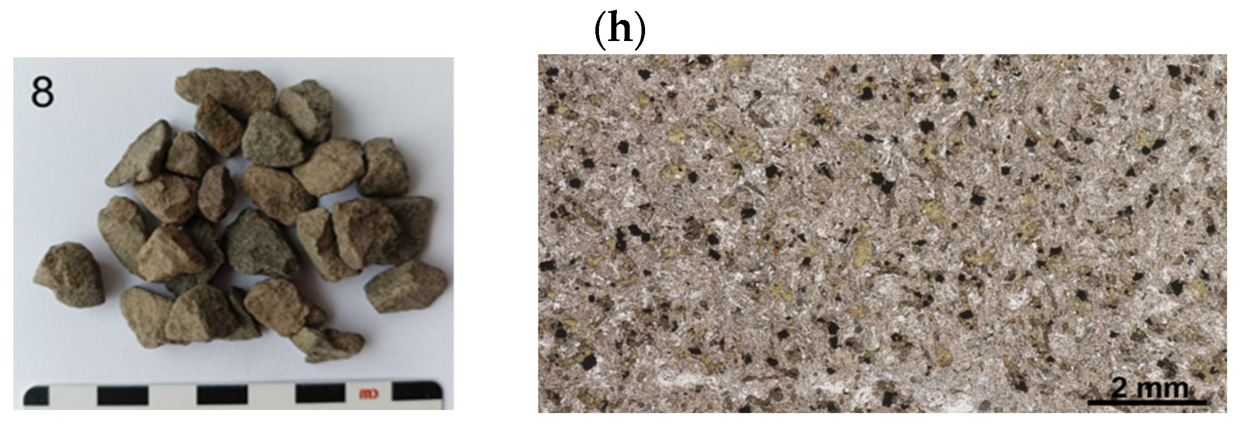
2.7. Polarising Microscope Examination

The petrographic examination was performed using a polarising microscope. The sampling process was performed using the quartz method in accordance with EN 932-1 [46]. Microscopic observations were made using eight prepared aggregate/rock slides on thin plates, i.e., uncovered polished (universal) thin plates, which allow observation under both polarised transmitted and reflected light.

This study aimed to describe the petrography of the aggregate/rock samples in terms of mineral composition, rock structure, and texture, determine the types of cement, describe the matrix, and determine the type of opaque minerals (observations under reflected light). Observations of aggregate/rock preparations were carried out with an Olympus BX-51 polarising microscope using polarised transmitted light. Photographic documentation was made using an Olympus SC18 camera.

3. Results

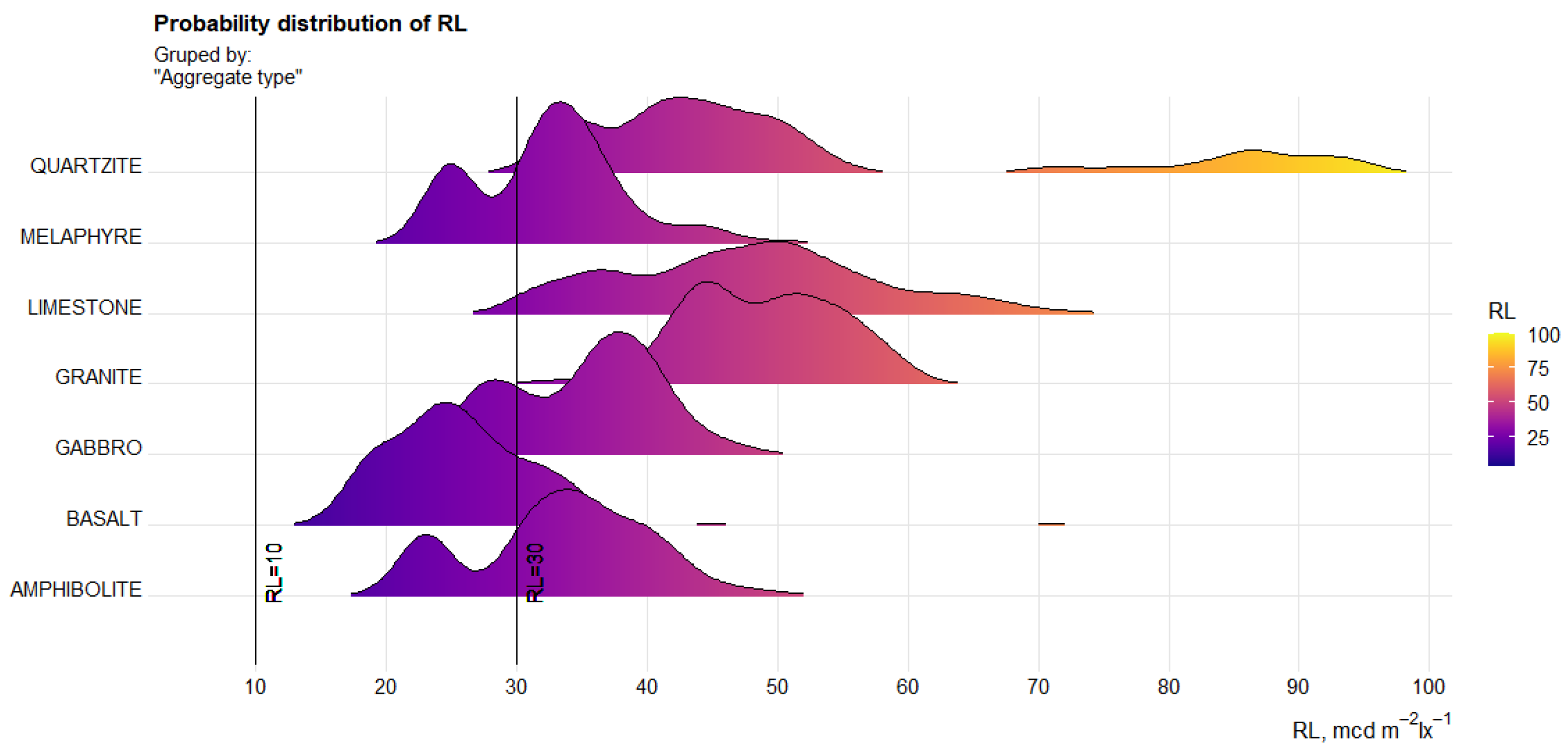
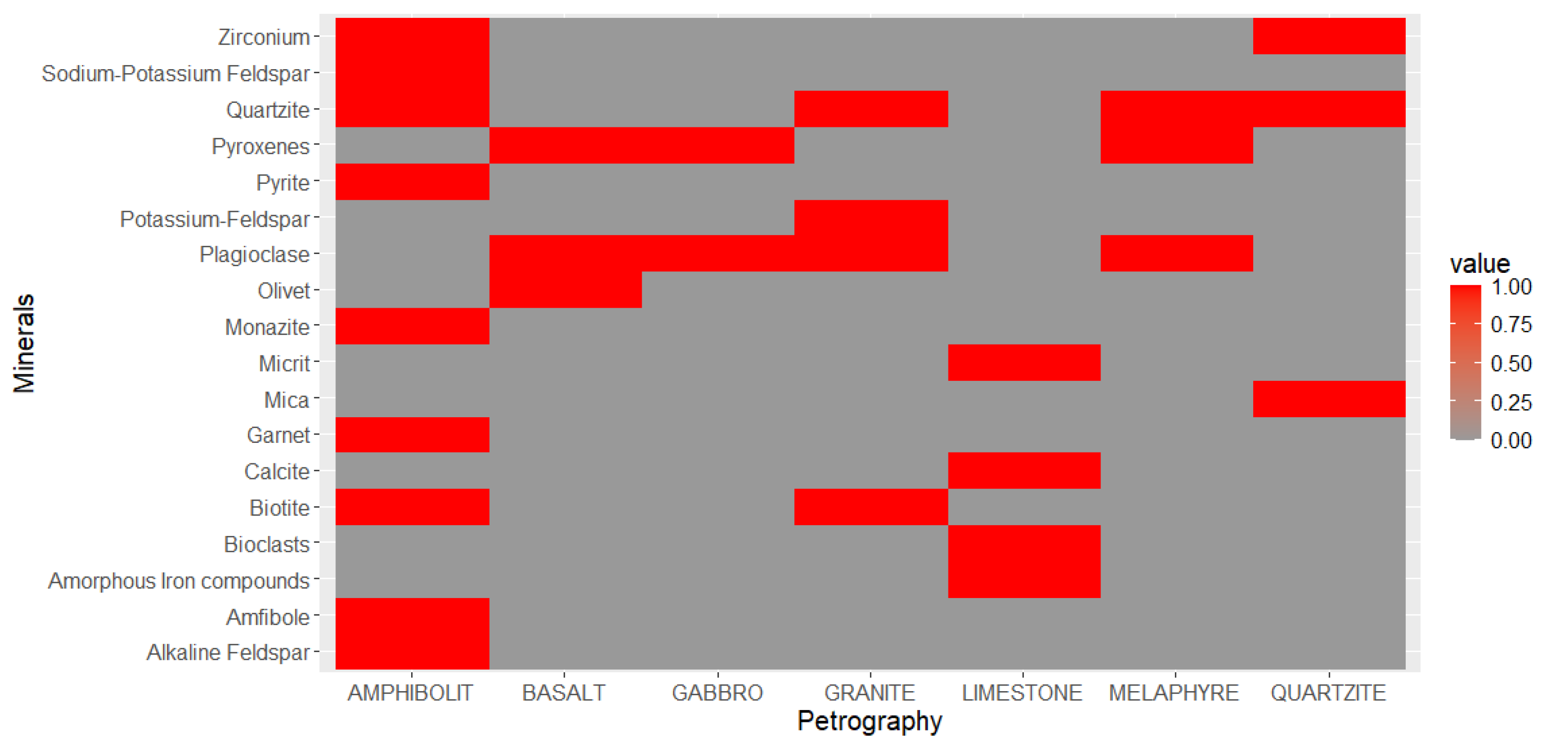
3.1. Luminance Coefficient Qd of the Aggregate vs. Mineralogical Composition

The detailed process of applying the boosted random tree (BT) algorithm required to predict the luminance ratio Qd is explained in detail in the article [15]. The results that fell within its scope provide the foundation for the search for further links that are the subject of this article. A summary of the test results, regarding the change in Qd in relation to aggregate type, is shown in Figure 7.

The unpublished Figure 7 shown represents the quality of the model fit by aggregate type. Taking into account the level of fractions used in Table 1, the quality of the representation of reality by the gradient-enhanced tree (BT) model was R² = 0.96 with relative error MAE = 4.3 mcd⋅m⁻²⋅lx⁻¹. Observing the results in Figure 7, it can be seen that the greatest dispersion of results was observed against the granite aggregate. With the results of the resulting BT model [15], a projection was made to illustrate the probability density of the predicted feature (Predicted Qd) by rock type. A graphical representation of the projection is shown in a ridge diagram developed in R (Figure 8).

Considering the value of the luminance coefficient, classifying the road pavement as black, Qd < 52 mcd⋅m⁻²⋅lx⁻¹, it must be concluded that basalt aggregate and melaphyre aggregate do not significantly affect the brightening of the pavement. In the case of gabbro rock aggregate, it does not allow for pavement brightening in certain cases. A much more favourable result in terms of magmatic rocks can be obtained by using aggregate from amphibolite and granite rocks. According to WT-2/2014, for surface illumination, aggregate with a Qd > 70 mcd⋅m⁻²⋅lx⁻¹_, should be used, i.e., in the examined set, all with a luminance coefficient close to the median value (Figure 8). In this group, the best results were obtained using quartzite sandstone (sedimentary) aggregate and limestone (sedimentary). In this group, very good results can be achieved using granite aggregate (igneous). However, it should be noted that all the rocks mentioned are formed differently and have different mineralogical structures. Therefore, it is to be expected that certain groups of minerals will be responsible for the luminosity factor Qd results obtained. However, before a mineralogical analysis is carried out, it is worth projecting the RL feature, i.e., the level of glare that the rocks generate from artificial light (car headlights). A graphical representation of the probability distribution of the measured RL feature is shown in Figure 9.

Figure 9 indicates the average observed level of road surface reflectivity RL falling within the range of 10 ÷ 30 mcd⋅m⁻²⋅lx⁻¹. Basalt aggregate, similar to the Qd, does not introduce any additional improvement in the reflectivity of the pavement. The amphibolite aggregate also has a reflectivity similar to the road surface, although the level of the Qd characteristic was significantly higher than the threshold value at which the pavement is considered ‘black’. A significant contribution to reflectivity was observed in the results of limestone, granite and quartzite sandstone aggregate. It is notable that among the results of the reflectance coefficient in artificial light for quartzite sandstone aggregate, there was a certain group of results in quartzite sandstone aggregate with an RL value >70 mcd⋅m⁻²⋅lx⁻¹. The observed singularity and the lack of a strong correlation between Qd and RL suggest that the mineralogical composition can definitely contribute to the understanding of the aggregate luminosity phenomenon.

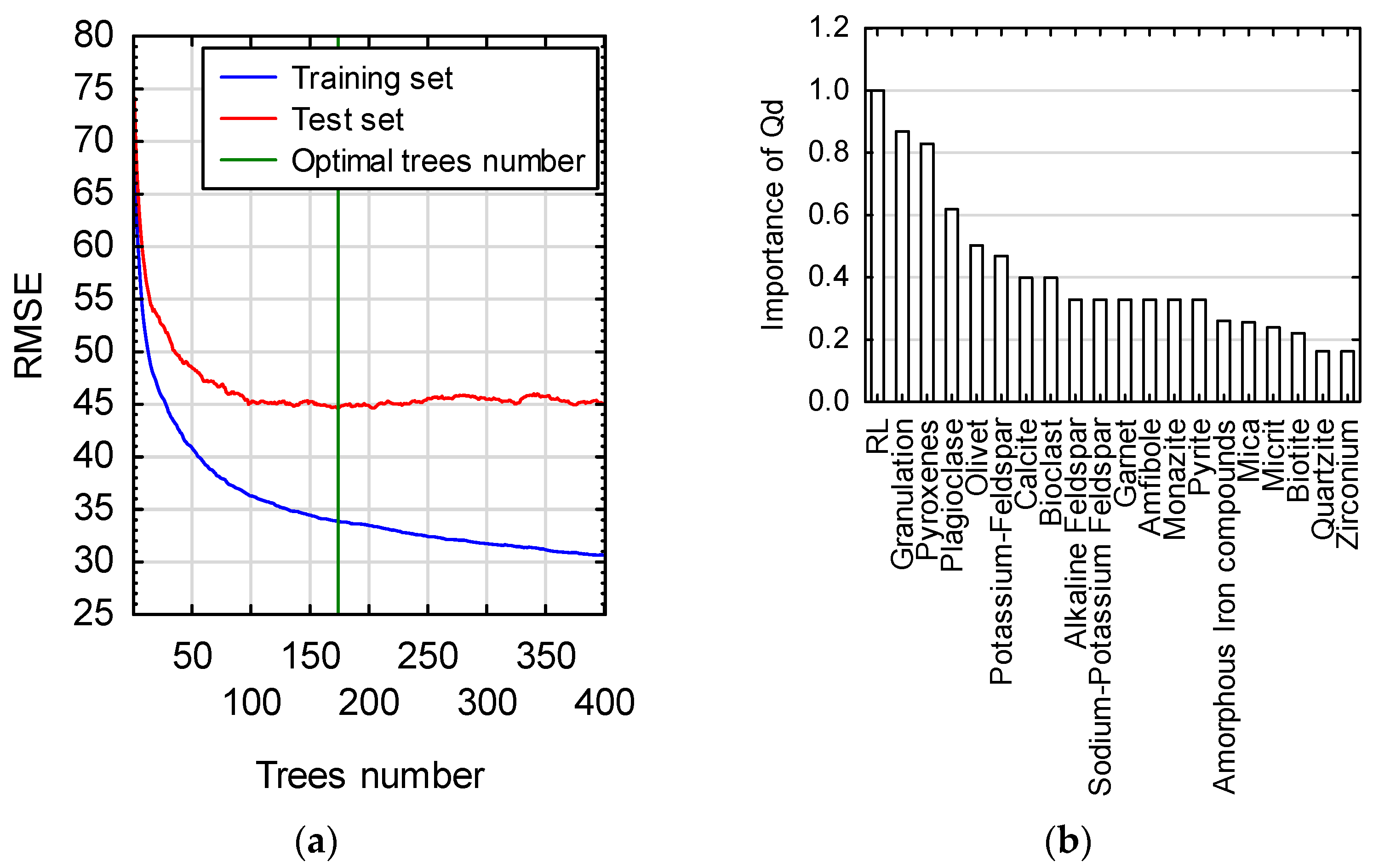
3.2. Regression Model of Aggregate Luminance Coefficient Taking Petrography into Account

The mineralogical tests carried out mostly correctly identified the type of aggregate/rock, although some variation was noted in the following aggregate sample type: amphibolite. All of them can be linked to the genesis of the deposit or the contamination effect caused by the aggregate production process. Photographs of the rocks used for the luminance ratio modelling, along with a view of the grinds, are shown in Figure 10.

The mineralogical evaluation was based on a petrographic examination of thin plates under a microscope suggesting the study [47]. The analysis was performed, excluding detailed geochemical analyses, using XRM microscopy. The state characterising the presence of a certain mineral was expressed by the symbol T, while its absence was expressed by the symbol N. The clustering results were performed using the dplyr and ggplot2 libraries in the R programming language [48,49]. A graphical visualisation of the results of the petrographic evaluation performed is shown in Figure 11.

Observing the results shown in Figure 11, it should be noted that the brightness of the aggregate does not depend on the presence of only one type of mineral. For sedimentary rocks (limestone), calcite was the dominant mineral, sedimentary rocks (quartzite sandstone) were dominated by quartz, and in igneous rocks, plagioclase and pyroxene were dominant. Observing the preliminary results, it was found that the contribution of quartz or calcite was definitely responsible for the high Qd level. In contrast, by simple elimination, the mineral mica was probably responsible for the high reflectivity state at night (RL). Thereby, its pearly sheen might have affected parameter RL. With the petrographic evaluation and the specified aggregate granulation available, an attempt was made to analyse their influence on the Qd characteristic. The petrographic analysis presented indicates that a single mineral was not attributed to a single rock type from which the aggregate range was produced. In the case of quartz, its occurrence was observed in granite and quartzite sandstone. Calcite, on the other hand, is characteristic of sedimentary rock (limestone). Therefore, there is a high probability that the formulation of the regression model based on the boosted tree (BT) technique will produce additional rules that describe the luminance phenomenon in the aggregate even more accurately and the resulting luminance coefficient value will have minimal estimation error.

The input file used to build the model was based on the data collected during the petrographic analysis and the data given in Table 1. The BT technique was chosen for the analysis in order to be able to refer to the results in the paper [15]. The optimal learning parameters were determined after taking the tuning process into account. The number of trees was limited to 400. During the construction of the BT model, a learning ratio η of 0.1 was used [50], while the ratio for randomising the learning samples in successive amplification steps was 0.5, suggesting the recommendations in the paper [51]. The final BT model was characterised by a tree structure with a maximum depth of 10 levels. It was very important to avoid ‘over-learning’ when learning the model, so the regularisation parameters α = 1, λ = 0 [52] were subjected to a fine-tuning process. The final model was built with a tree count of 174. The analyses obtained were performed using Statistica [51]. The learning flow and parameter validity, using the RMSE metric, are shown in Figure 12.

Note the results of the importance indicators. The predictor validity graph (Figure 12b) suggests that the feature related to the reflective properties of the aggregate illuminated by car headlights had the greatest influence on the formulated set of rules for the learning process. In addition, the aggregate grain size had a very important influence on the discriminatory rules obtained. There is a logical rationale for this, as a higher proportion of fine aggregate results in an increase in its volumetric proportion in the composition of the mineral mixture and an increase in its specific surface area. With regard to the mineralogical composition, the percentage of minerals such as pyroxene, plagioclase, and olivine mainly determined the distribution of the aggregate luminance value (Qd). Of the mineral assemblage, calcite (limestone and quartzite) and potassium feldspars (granite) played an important role in shaping the high clarity of the aggregate. It can be added that these minerals are mainly colourless, white minerals with a glassy shine. The analysis carried out was complemented by a variability graph developed based on the predicted results of the Qd trait using the BT model. The diagram below is shown in Figure 13.

Observing the results in Figure 13, it should be noted that the presence of a pyroxene-type mineral strongly divides the whole community into dark- and light-coloured aggregates according to the classification of the report [52]. According to its results, an aggregate with a luminance ratio of Qd < 70 mcd⋅m⁻²⋅lx⁻¹ is an aggregate that is considered dark. It should be noted that pyroxene is a major component of deep-sea magmatic rocks, e.g., basalt. A very high Qd value was obtained for rocks containing calcite, which is the main component of a sedimentary rock such as limestone. The same picture is given by rules characterised by the presence of plagioclase and quartz, i.e., granitic rock. A very interesting observation is the interaction of quartz and mica, the minerals found in some grains of quartzite sandstone aggregate. The interaction of these two minerals allowed for achieving Qd > 100 mcd⋅m⁻²⋅lx⁻¹, which means aggregates with high lightening values for the potential road surface. The presence of the mineral mica (lat. ‘shine’) has already been signalled as improving the reflectivity of the aggregate in artificial light. In order to compare the effectiveness of the modelling including petrographic analysis, the results of the model including mineralogical composition were compared with the results provided by the model included in the work [15]. The following three metrics were used for benchmarking:

• Root mean square error (RMSE);
• R-squared (R²);
• Mean absolute error (MAE).

The results of the comparison are shown in

Table 4. Result of fitting the BT model taking into account the analysis of the petrography of the variable Qd.

Metrics	BT Model with Petrography Analysis	The BT Model Included in the Paper by Mazurek et al. [15]
R2	0.97	0.96
RMSE, mcd⋅m−2⋅lx−1	5.8	6.2
MAE, mcd⋅m−2⋅lx−1	4.1	4.3

.

Observing the results in Table 4, it should be noted that the degree of improvement in the prediction of the Qd trait value compared to the results in the [15] paper increased slightly (MAE decrease of only 0.2 mcd⋅m⁻²⋅lx⁻¹). The consideration of the mineralogical composition was of greater importance in the cognitive context of the aggregate luminance phenomenon. In the regression approach analysed, expressing the petrographic characteristics using only the name of the rock from which the aggregate was produced can be considered sufficient from the point of view of the predictive quality of the model. It is likely that extending the research programme to include rock chemistry would have a far greater impact on the accuracy of aggregate luminance ratio prediction.

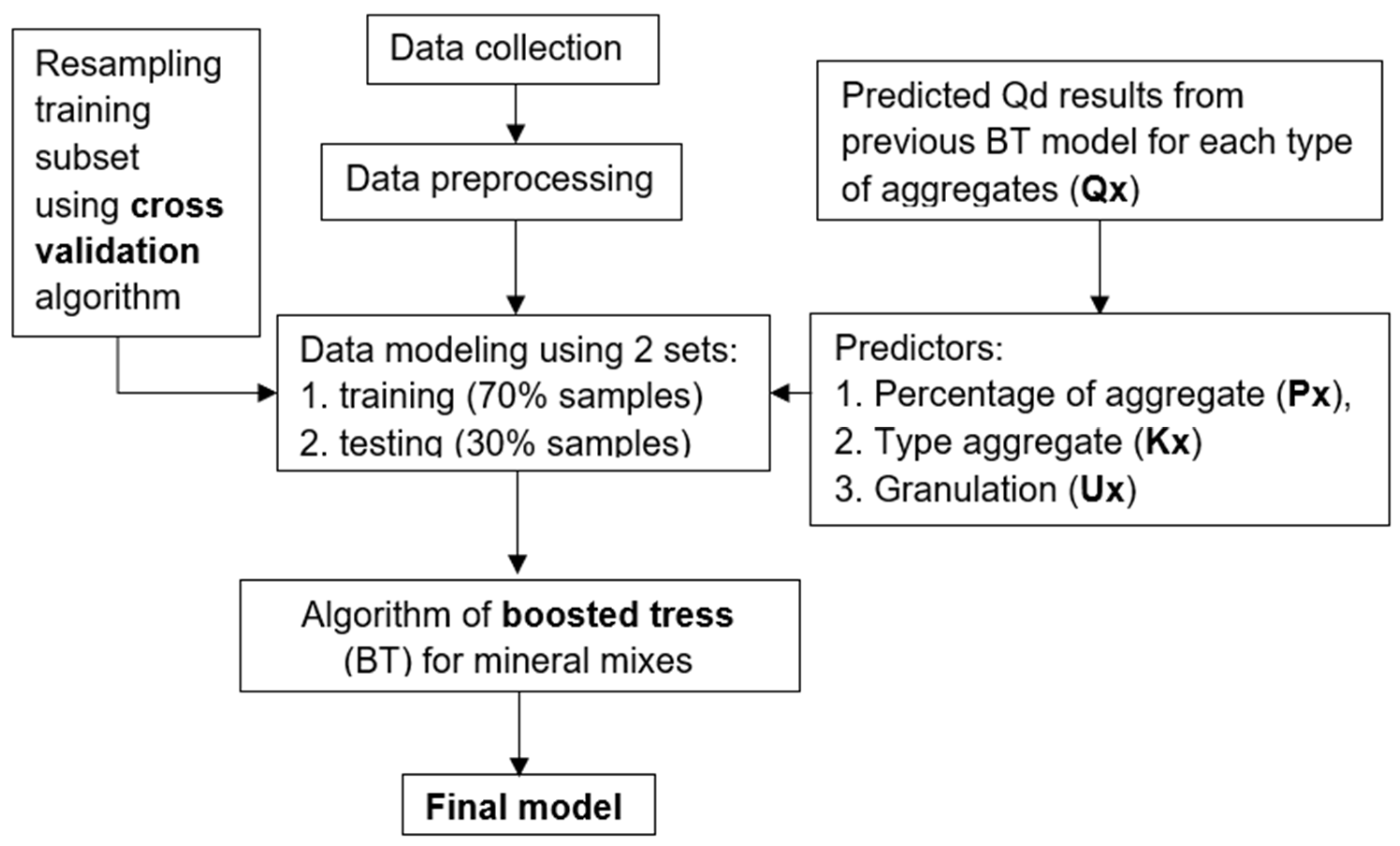
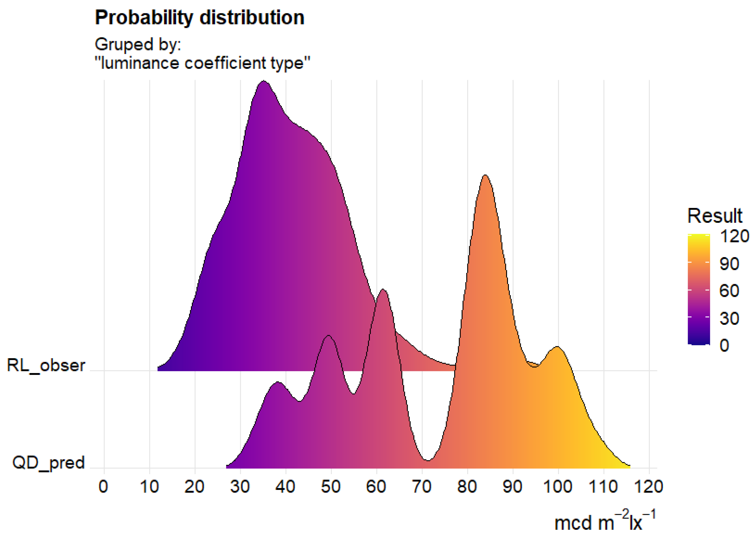
3.3. Regression Model of the Luminance Ratio for the Mineral Mixture

The modelling of the luminance coefficient value Qd of the mineral mixture was based on the conclusions and results of the luminance coefficient modelling for the aggregate. The model developed in Section 3.2 was selected for further analysis as it allowed for a reduction in the forecast error attributed to the aggregate. However, it should be borne in mind that the inclusion of a model incorporating the results of the mineralogical analysis will increase the quality of the luminosity ratio prediction but will definitely reduce its usefulness from the point of view of practical applications. This is due to the fact that mineralogical analyses are rarely performed in the road industry for a given aggregate. Independently of this, the experience and results of the model given in the paper [15] can also be used for the analysis in the absence of detailed petrographic investigations.

As mentioned before, the structure of the mineral mix input set was based on the use of designed compositions of 30 mineral mixes for real road pavements loaded with medium traffic of category KR5-7 (7.3∙10⁶ ÷ 52∙10⁶ ESAL). All the mineral mixtures were designed for the pavement-wearing course made of asphalt concrete and stone mastic asphalt. All mineral mixtures had to comply with the grain size requirements applicable in Poland, according to WT-2/2014 [43]. The introduction of such conditions ruled out the possibility of using a single type of aggregate, as its crumb pile would have prevented the compaction of a mineral and asphalt mixture (mma) made with it under real-world conditions. Another limitation was due to the acidity of the rocks, i.e., the silica content (SiO₂). The use of acid rock, e.g., quartzite sandstone and granite, would result in a loss of the required water resistance of the mma due to the low adhesion of these rocks to the asphalt. On the other hand, the use of an aggregate with a high adhesion with limestone will not provide the required value of resistance to fragmentation (Los Angeles coefficient) LA < 40. Taking all conditions into account, the mineral mixture consisted of three to four aggregates of different granulation types (Kx). The advantage of doing it this way was that it was possible to replicate the actual mineral and asphalt mixtures that were used to produce the mma and thus the rules that were specified in the model applied to real conditions. The knowledge-containing model developed in the previous chapter for predicting the luminance coefficient of the aggregate (Qx) was implemented in the modelling of the luminance coefficient of the mineral mixer in the form of an XML exchange file. The number of results in the input set was 450 and its structure is shown in

Table 5. Structure of the input set for the determination of Qd of the mineral mixture.

Quantitative Dependent Variable
Luminance ratio in diffuse light (Qd)	mcd⋅m−2⋅lx−1
Surface reflectance (RL)	mcd⋅m−2⋅lx−1
Quantitative independent variable (quantitative predictor)
The luminance coefficient Qd for the aggregate (value derived from model described in Section 3.2), Qx	mcd⋅m−2⋅lx−1
Percentage fraction of aggregate, Px	%
Qualitative independent variable (qualitative predictor)
Aggregate grain size, Ux	0/2, 2/5, 2/8, 5/8, 8/11
Type of aggregate, Px	Limestone, Quartzite Sandstone, Melaphyre, Granite, Amphibolite, Basalt, Gabro
Number of fractions in mm, Kx	from 3 to 4

.

When building the model, the finest fraction of the U1 aggregate with a grain size of 0/2 was not included. This type of fraction would definitely falsify the luminance ratio result. In addition, the fine aggregate fractions are surrounded by the asphalt to form a mastic (fine aggregate and asphalt binder); therefore, it would be unreasonable to leave this fraction in mm. Nevertheless, they are taken into account during the design of the mm composition. An algorithm for proceeding to model the luminance ratio of the mineral mixture in the form of a flowchart is shown in Figure 14.

The task at hand was new, so to select an appropriate DM technique, the tool provided by the Statistica package included in the Data Miner Recipes module was used. Its operation and outcome should be seen primarily as a feasibility study as to the integrity of the dataset, as well as an indication of the technique that is likely to be most effective for luminance ratio prediction. The following four DM regression techniques were initially selected for the task:

• Random forest (RT);
• Neural network (ANN);
• Reinforced random trees (BT);
• Classical random trees (C&RT);
• Multi adaptive regression splines (MARS).

The best machine learning model had to exhibit the smallest RMSE value among their models. In the case of the MARS model, it was required to give quality labels to some of the variables, and this technique ultimately proved unsuccessful. The C&RT technique also failed to produce a satisfactory prediction result. A summary of the preliminary results is shown in

Table 6. A preliminary review of machine learning techniques for the prediction of the Qd feature of a mineral mixture.

Name	Mean Sum of Squares of Residuals (RMSE), Learning	Correlation, Learning	Selection for Evaluation
Reinforced trees	35.69	0.93	TRUE
Neural network	37.43	0.92	TRUE
Random forest	91.5	0.85	TRUE
C&RT	158.61	0.71	FALSE
MARS	-	-	FALSE

.

Of all the learning techniques, the reinforced tree (BT) algorithm was selected for further evaluation. The results of the quality of fit obtained took into account the use of all the results in the set without dividing them into a teaching and test set. The modelling function has undergone a fine-tuning process. This process was performed using the caret library available in the R programming language, which allows any modelling function to be effectively tuned. The following parameters were taken into account in the fine-tuning process:

• nrounds—controls the maximum number of iterations;
• η—controls the learning rate;
• γ—controls regularisation (or prevents overfitting);
• max depth—controls the depth of the tree;
• min. child weight—refers to the minimum number of instances required in a child node;
• subsample—controls the number of samples (observations) supplied to a tree.

The tuning process consisted of iterating specific combinations of BT model parameters (xgbTree method) considered in a fixed parameter grid using also a cross-check. Cross-validation was introduced to avoid excessive overfitting of the model built from the training set. Then, after a time-consuming calculation process, the result was presented in the form of a vector of parameter values at which the model achieved the highest efficiency. The RMSE metric was used as a criterion for selecting the best model. A graph representing an extract of the RMSE results from the parameter tuning process is shown in Figure 15.

Finally, the best model, with the lowest RMSE value, after the tuning process was carried out, was characterised by the parameters that are given in

Table 7. Parameter values after the BT model tuning process (learning set).

η	Max Depth	γ	Subsample	Min. Child Weight	Nrounds	RMSE	R2	MAE
0.05	5	5	0.5	3	120	7.1	0.82	5.7

.

It should be noted that the test set was used to verify the value of nrounds, the value of which was finally set as 120. Further increases in the nrounds parameter led to overfitting of the BT model. The quality of the model fit containing the results of the entire set (learning and test set) between the feature Qd_obs (observed values) and the set of predicted values Qd_predic was R² = 0.87, MAE = 4.4 mcd⋅m⁻²⋅lx⁻¹ and RMSE = 5.7 mcd⋅m⁻²⋅lx⁻¹. The quality results obtained were considered satisfactory. It was also important to assess the quality of the model by analysing its structure by means of a validity chart of the variables. On the basis of these, it is possible to assess which variable has the greatest influence on the distribution of trees and the relationship between them and allows practical conclusions to be drawn. Variable importance plot and quality of fit model Qd_predic vs. Qd_obs are shown in Figure 16.

Observing the results in Figure 16b, it should be noted that the luminosity coefficient of aggregate fraction (component) No. 2 and No. 3 (Q2, Q3) had the greatest influence on the determination of rules when building the BT model. The percentages of fractions two (P2) and three (P3) were also very significant. An interesting note comes from the assessment of the importance of the following feature interactions: K3-Basalt and K3-Quartize. This was most likely due to the presence of pyroxene in the aggregate, which clearly separates the community into light and dark aggregates (as per Figure 8). Thus, the presence of these rocks in fraction 3 will significantly affect the final luminance value of the mineral mixture. The granularity of the grain size (Ux) was also important, although no longer as important as the characteristics mentioned. In order to understand the structure of the set, partial dependence plots were used, the purpose of which was to determine the strength of the influence of a given variable while marginalising the influence of the others and expressing it in terms of an average value of the Qd characteristic (denoted as yhat). It is a useful analytical tool, especially when we are interested in the logical justification of the presence of variables, and when we are looking for general conclusions of a practical nature. The information in Figure 16 is developed and graphically presented in Figure 17 by type of component in the mineral mix (excluding component 1).

Due to the small effect of aggregate granulation on the Qd value (Figure 16b), a subgraph (Ux) was not made for this variable. In contrast, the influence of the characteristics Kx, Qx, and Px was much more significant. Before carrying out the analysis, it is useful to indicate what granularity each mineral mixture component had. Aggregate No. 2 (appropriately described by features K2, Q2, P2) could occur as a fraction, 2/5 or 2/8, aggregate No. 3 could occur as a fraction, 2/8, 5/8, while No. 4 could occur as a fraction 8/11 or no fraction. An analysis of Figure 17a indicates the greatest influence on the high brightness of the granite aggregate in fraction No. 2 (K2). In addition, the introduction of quartzite sandstone aggregate as a component of K2 and K3 had a very favourable effect on the luminance coefficient of the mineral mixture (mm). The opposite was the basalt aggregate, the presence of which had the opposite effect. It was much more interesting to find out at what average percentage of luminous aggregate the effect of an increased mm luminance value could be obtained, depending on the component type. Figure 17b,c show that the proportion of Q2 aggregate with a fraction of 2/5 or 2/8 above 40% and with a luminance coefficient Qd > 70 mcd·m⁻²·lx⁻¹ caused a sudden increase in the Qd mm characteristic (increase in yhat value). Similarly, in the case of ingredient No. 4 (fraction 8/11), an increase in its share >60% (P4) in the mm composition containing bright aggregate caused a significant increase in the brightness of mm. In component No. 3 (fractions: 2/8 or 5/8), the greatest impact on the luminance coefficient mm was caused by a percentage share from 25% to 50%, and only then when the aggregate from Qd > 80 mcd·m⁻²·lx⁻¹ was used. Only quartzite sandstone or granite aggregate could provide such a result. Ingredient No. 4, i.e., aggregate with a fraction of 8/11, only mattered when its share was >60%. This result is justified when its specific surface area is taken into account. Aggregate of this grain size will definitely have a lower specific surface area than the finer fractions found in components 2 and 3. Consequently, the coarsest fraction (No. 4) will have far less impact on the luminance ratio than the fine fraction. However, it should be remembered that the coarse fractions are responsible for the high resistance of the mineral–asphalt mixture (mma) to permanent deformation. Therefore, optimising the composition of the mma for the sake of maintaining high resistance to permanent deformation is likely to reduce the potential of the light aggregate to lighten the pavement. The luminance ratio can also be determined from other assessments. The value of QD can also be determined by using the weighted mean according to Formula (4), as follows:

$${\mathrm{Q}\mathrm{d}}_{\mathrm{m}\mathrm{e}\mathrm{a}\mathrm{n},\mathrm{w}\mathrm{e}\mathrm{i}\mathrm{g}\mathrm{h}\mathrm{t}\mathrm{e}\mathrm{d}}=\frac{{\mathrm{P}}_i{\mathrm{Q}}_i+\dots +{\mathrm{P}}_n{\mathrm{Q}}_n}{\sum _{\mathrm{i}=\mathrm{n}}^{\mathrm{n}}{\mathrm{P}}_i}$$

(4)

where Qd_{mean,weighted} is the weighted mean of luminance coefficient mm and P_i is the percentage of aggregate in the i-th component mm, luminance coefficient of an aggregate of the i-th component. The results of the projected Qd_{mean.weighted} value are presented graphically in the summary of results shown in Figure 18.

The quality of the model fit based on the Qd_{mean.weighted} calculation decreased from R² = 0.87 (based on the BT model) to 0.71. This decrease can be explained by the variation in the weighted average value of 12%. However, by observing deviations from the line of proportionality, the model using a weighted average is unable to explain many of the outliers that arose during the analysis. This is because the distribution of the aggregate trait Qd did not have a normal distribution and is characterised by multimodality (Figure 8). Thus, the central measures used in the parametric tests will not allow for an adequate prediction of the results of such a complex quantity as the luminance factor Qd of the mineral mixture, and the resulting residuals will not meet the homoscedasticity condition.

It should be made clear at this point that the interpretation of the results obtained from the BT model relates only to the set of aggregates used for the analysis, and the relationships occurring between the components also resulted from the regulations imposed by the technical requirements WT-1/2014 for aggregates and WT-2/2014 for the composition of mineral mixtures in force in Poland. However, there is nothing to prevent this model from being further evaluated using other mineral compositions subject to different compositional rules. The resulting set of results covers a wide spectrum of the luminance coefficient Qd, as well as the labelled RL coefficient. In summary, the probability distribution of the results occurring in the experiment is shown in Figure 19.

The range of luminance ratio results predicted by the Qd_predic model is between 28 mcd⋅m⁻²⋅lx⁻¹ and 116 mcd⋅m⁻²⋅lx⁻¹. In contrast, the RL factor most often obtained a value in the range 35 ÷ 40 mcd⋅m⁻²⋅lx⁻¹ during the tests. It is the intention of the authors to further validate and calibrate the developed model predicting the luminance coefficient Qd of the aggregate, as well as the mineral mixture. In the next step, the relationships between the aggregate, mineral mix, and mineral–asphalt mixture subjected to wear and tear and the luminance coefficient will be sought. The main objective is to build a DM model to predict the luminance ratio at the design stage of the mineral–asphalt mix.

4. Conclusions

It should be noted that aggregate resources are not inexhaustible. Therefore, their availability on the market will decrease over time. Currently, mines regulate the amount of extracted aggregate using the principle of sustainable development. Therefore, the amount of aggregate that is extracted depends on the forecasted demand in the long-term perspective. Moreover, it should also be taken into account that in the bituminous mixtures, there are also recycled aggregates, which will also require the assessment of properties and affect the pavement luminance value. Therefore, an effective numerical model will definitely facilitate their selection for the composition of mineral mixtures. The modelling process presented here proved that a very good representation of the luminance coefficient of the aggregate and the mineral mixture made with it can be obtained using machine learning techniques. Thus, the ability to predict the luminosity of a mineral mix will allow, at the design stage of a mineral and asphalt mix, the composition of the mix to be selected in such a way as to achieve the maximum level of luminosity while maintaining the required mechanical characteristics. The research and analysis resulted in the following conclusions:

• The use of machine learning techniques is an excellent tool for modelling the luminance ratio of aggregates and mineral mixtures;
• The inclusion of a thorough petrographic analysis in the prediction of the aggregate luminance ratio resulted in some improvement in the prediction of the aggregate luminance ratio compared to the case in which its influence was expressed solely by the name of the aggregate;
• The mineral that was most decisive in the division between dark and light aggregates was pyroxene, which was characteristic of igneous rocks such as basalt and melaphyre;
• The mineral that is probably responsible for the increased reflectivity (nighttime visibility) was mica found in quartzite sandstone, among others;
• The best results in terms of surface brightening with Qd > 70 mcd·m⁻²·lx⁻¹ were obtained with quartzite sandstone (sedimentary) and granite (igneous), in which the quartz mineral predominated. In contrast, the sedimentary rock class was limestone, which contained mainly calcite;
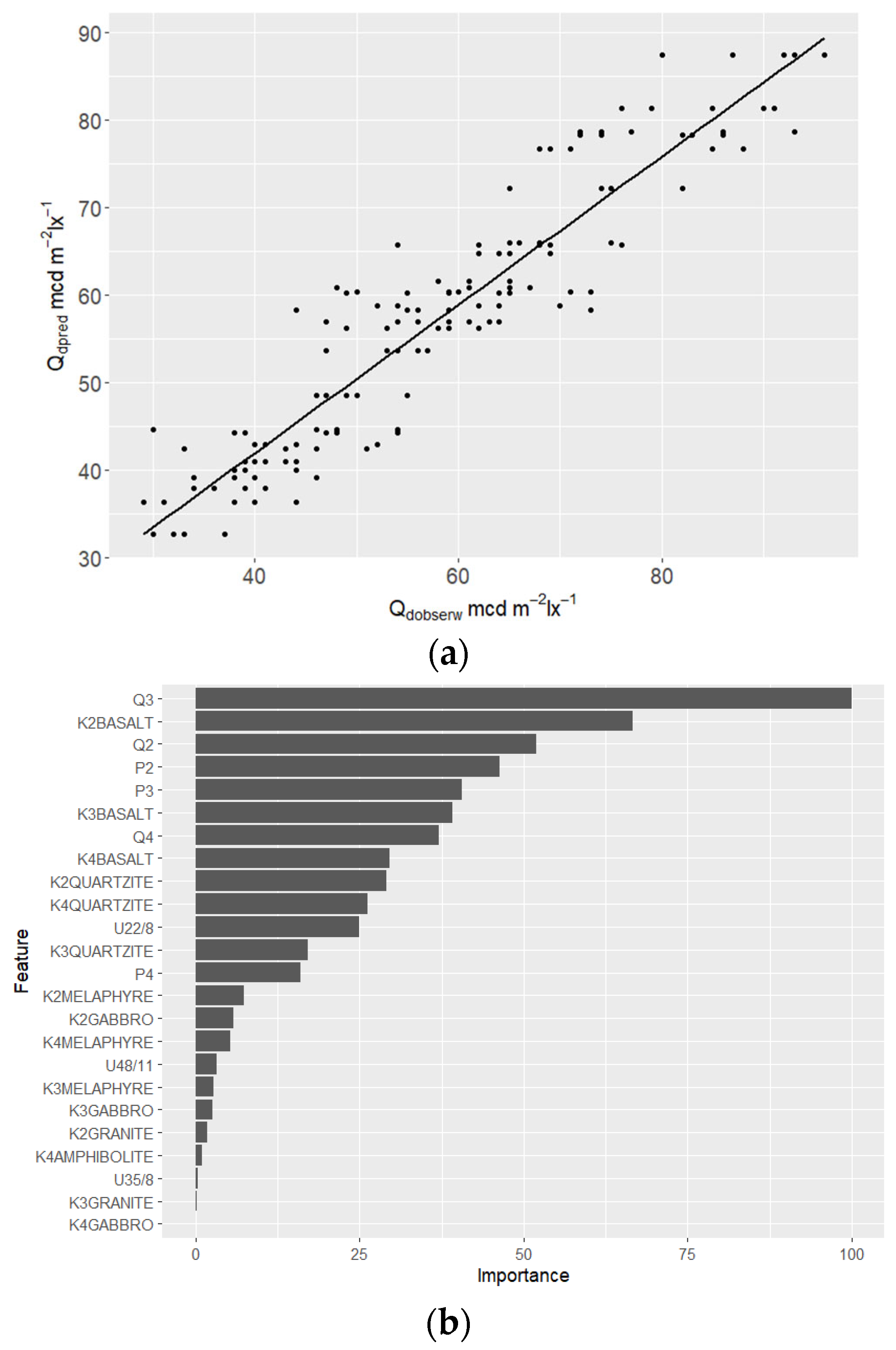
• The amplified random tree (BT) technique used, supported by additional tuning and cross-check (test set) procedures, allowed the construction of a stable BT model characterised by an absolute error of MAE = 5.7 mcd⋅m⁻²⋅lx⁻¹ and RMSE = 4.4 mcd⋅m⁻²⋅lx⁻¹. The correlation value of the predicted values against the observed values was 87%. The present model effectively eliminated the singularities present, minimising outliers;
• The greatest influence on the construction of relationships in the amplified random tree model was the percentage and value of the luminance ratio of mainly the 2/5 and 2/8 fractions;
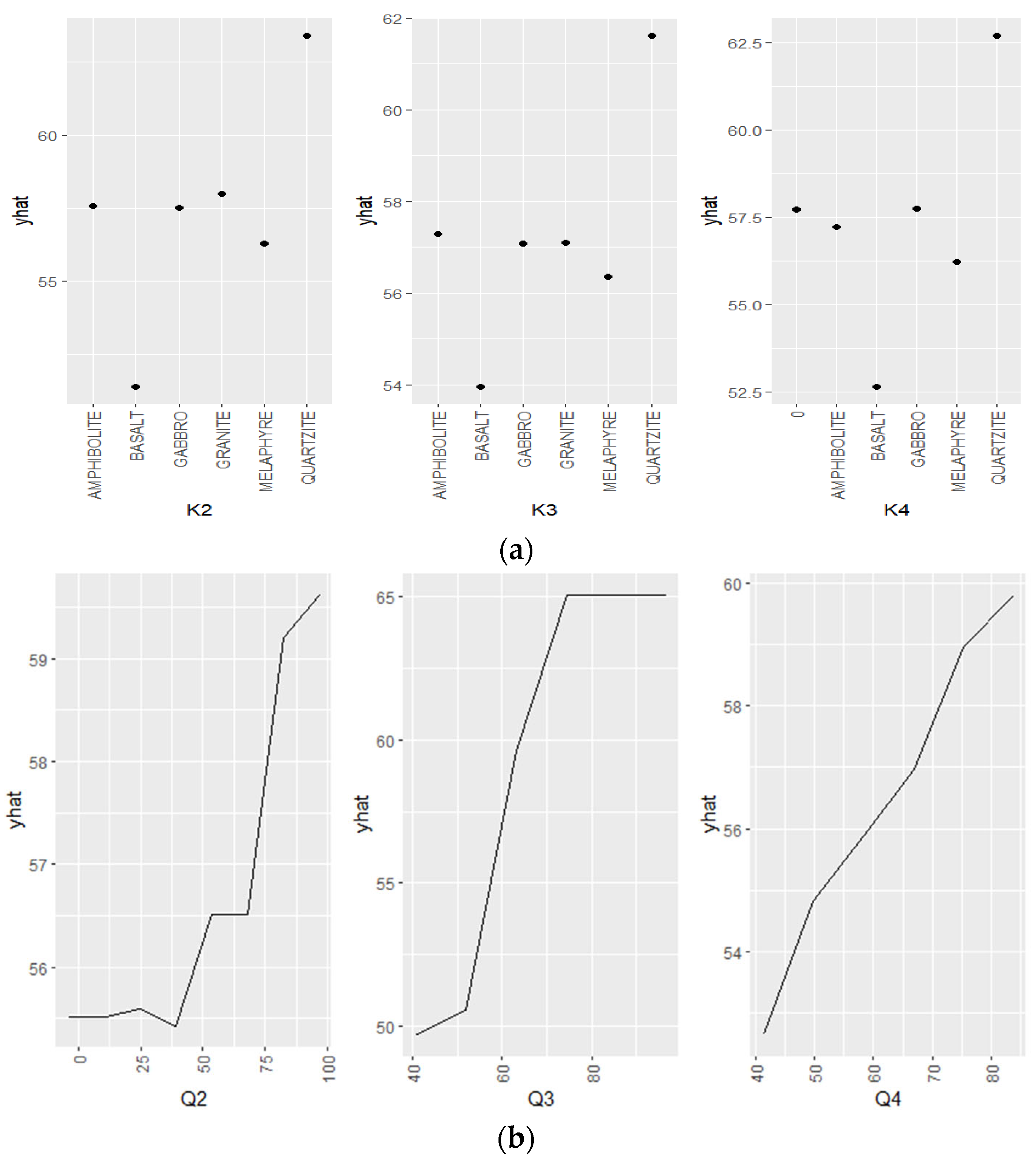
• An analysis of the individual impact of variables on the variability of the predicted BT model indicates that the use of light aggregate fractions with a grain size of 2/5 in quantities >40% or light aggregate 8/11 in quantities of 60% provides a rapid improvement in the degree of lightening of the mineral mixture;
• The presence of 5/8 fraction quartzite sandstone showed the best results in terms of brightening the mineral mix. In contrast, a sharp decrease in the luminance coefficient was recorded in mineral mixtures in which basalt aggregate occurring in the 5/8 fraction was used;
• It is important to note that the machine learning technique adopted was chosen as the most effective due to its quality in predicting the luminance coefficient. This does not mean that other techniques will not be effective. The development of artificial intelligence can provide new models with architectures that will be decidedly better than the BT technique. The authors of this publication are still working on improving the machine learning model.

References

1. Filipczyk, M.; Kukielska, D. Bright and Bleached Surfaces. Theory and Practice. Min. Sci. 2016, 23, 17–22, ISSN 2300-9586. [Google Scholar] [CrossRef]
2. Onaygil, S. Road Lighting Calculations; CIE Technical Committee 4-15 of Division 4 “Transportation and Exterior Applications”: Vienna, Austria, 2000; ISBN 978-3-901906-54-1. [Google Scholar]
3. Strbac-Hadzibegovic, N.; Strbac-Savic, S.; Kostic, M. A New Procedure for Determining the Road Surface Reduced Luminance Coefficient Table by On-Site Measurements. Light. Res. Technol. 2019, 51, 65–81. [Google Scholar] [CrossRef]
4. Van Bommel, W.J.M.; Burghout, F.; Cobb, J. Road Surfaces and Lighting: Joint Technical Report CIE/PIARC; CIE Central Bureau: Vienna, Austria, 2008; ISBN 978-3-901906-72-5. [Google Scholar]
5. Bodmann, H.W.; Schmidt, H.J. Road Surface Reflection and Road Lighting: Field Investigations. Light. Res. Technol. 1989, 21, 159–170. [Google Scholar] [CrossRef]
6. Van Tichelen, P.; Jansen, B.; Geerken, T.; Vanden Bosch, M.; Van Hoof, V.; Vanhooydonck, L.; Vercalsteren, A. Final Report Lot 9: Public Street Lighting; European Commission: Brussels, Belgium, 2007. [Google Scholar]
7. Adrian, W.; Almasi, S.; Arens, J.B. Calculation and Measurement of Luminance and Illuminance in Road Lighting: Computer Program for Luminance, Illuminance and Glare, 2nd ed.; Internationale Beleuchtungskommission, Ed.; Technical Report; Reprint; CIE Central Bureau: Vienna, Austria, 1990; ISBN 978-92-9034-030-0. [Google Scholar]
8. Zieja, M.; Wesołowski, M.; Blacha, K.; Iwanowski, P. Analysis of the Anti-Skid Properties of New Airfield Pavements in Aspect of Applicable Requirements. Coatings 2021, 11, 778. [Google Scholar] [CrossRef]
9. Šrámek, J.; Kozel, M.; Remek, L.; Mikolaj, J. Evaluation of Bitumen Modification Using a Fast-Reacting SBS Polymer at a Low Modifier Percentage. Materials 2023, 16, 2942. [Google Scholar] [CrossRef] [PubMed]
10. Ylinen, A.-M.; Pellinen, T.; Valtonen, J.; Puolakka, M.; Halonen, L. Investigation of Pavement Light Reflection Characteristics. Road Mater. Pavement Des. 2011, 12, 587–614. [Google Scholar] [CrossRef]
11. PKN-CEN/TR 13201-1:2016-02; Road Lighting. The Polish Committee for Standardization: Warsaw, Poland, 2016.
12. Sørensen, K.; Nielsen, B. Road Surfaces in Traffic Lighting. 1974. Available online: https://trid.trb.org/view/37817 (accessed on 18 June 2024).
13. Bonomo, M.; Burghout, F.; Hautala, P.; Marinier, J.C.; Simons, R.H.; Stark, R.E.; Stockmar, A.; Vermeulen, J. Design Methods for Lighting of Roads; Internationale Beleuchtungskommission, Ed.; CIE Central Bureau: Vienna, Austria, 1999; ISBN 978-3-900734-92-3. [Google Scholar]
14. Qin, L.; He, S.; Yang, D.; Leon, A.S. Proposal for a Calculation Model of Perceived Luminance in Road Tunnel Interior Environment: A Case Study of a Tunnel in China. Photonics 2022, 9, 870. [Google Scholar] [CrossRef]
15. Mazurek, G.; Bąk-Patyna, P. Application of Data Mining Techniques to Predict Luminance of Pavement Aggregate. Appl. Sci. 2023, 13, 4116. [Google Scholar] [CrossRef]
16. Montgomery, D.C. Design and Analysis of Experiments, 8th ed.; John Wiley & Sons, Inc: Hoboken, NJ, USA, 2013; ISBN 978-1-118-14692-7. [Google Scholar]
17. Rebelo, F.J.; Martins, F.F.; Silva, H.M.; Oliveira, J.R. Use of Data Mining Techniques to Explain the Primary Factors Influencing Water Sensitivity of Asphalt Mixtures. Constr. Build. Mater. 2022, 342, 128039. [Google Scholar] [CrossRef]
18. Gong, H.; Sun, Y.; Mei, Z.; Huang, B. Improving Accuracy of Rutting Prediction for Mechanistic-Empirical Pavement Design Guide with Deep Neural Networks. Constr. Build. Mater. 2018, 190, 710–718. [Google Scholar] [CrossRef]
19. Guo, X.; Hao, P. Using a Random Forest Model to Predict the Location of Potential Damage on Asphalt Pavement. Appl. Sci. 2021, 11, 10396. [Google Scholar] [CrossRef]
20. Phan, T.M.; Jang, M.-S.; Seo, J.-W.; Yoon, J.-H.; Park, D.-W.; Minh Le, T.H. Impact of Air Voids and Environmental Temperature of Asphalt Concrete on Black Ice. Road Mater. Pavement Des. 2023, 24, 91–106. [Google Scholar] [CrossRef]
21. Fakhri, M.; Shahni Dezfoulian, R. Pavement Structural Evaluation Based on Roughness and Surface Distress Survey Using Neural Network Model. Constr. Build. Mater. 2019, 204, 768–780. [Google Scholar] [CrossRef]
22. Gopalakrishnan, K.; Agrawal, A.; Ceylan, H.; Kim, S.; Choudhary, A. Knowledge Discovery and Data Mining in Pavement Inverse Analysis. Transport 2013, 28, 1–10. [Google Scholar] [CrossRef]
23. Bashar, M.Z.; Torres-Machi, C. Performance of Machine Learning Algorithms in Predicting the Pavement International Roughness Index. Transp. Res. Rec. 2021, 2675, 226–237. [Google Scholar] [CrossRef]
24. Tong, Z.; Gao, J.; Sha, A.; Hu, L.; Li, S. Convolutional Neural Network for Asphalt Pavement Surface Texture Analysis: Convolutional Neural Network. Comput.-Aided Civ. Infrastruct. Eng. 2018, 33, 1056–1072. [Google Scholar] [CrossRef]
25. Corte-Valiente, A.; Castillo-Sequera, J.; Castillo-Martinez, A.; Gómez-Pulido, J.; Gutierrez-Martinez, J.-M. An Artificial Neural Network for Analyzing Overall Uniformity in Outdoor Lighting Systems. Energies 2017, 10, 175. [Google Scholar] [CrossRef]
26. Kazanasmaz, T.; Günaydin, M.; Binol, S. Artificial Neural Networks to Predict Daylight Illuminance in Office Buildings. Build. Environ. 2009, 44, 1751–1757. [Google Scholar] [CrossRef]
27. Kayakuş, M.; Üncü, İ.S. Basketbol Salonlarının Parıltısının Makina Öğrenme Yöntemleriyle Tahmini. Düzce Üniversitesi Bilim Ve Teknol. Derg. 2020, 8, 2468–2479. [Google Scholar] [CrossRef]
28. WT-1 Kruszywa Do Mieszanek Mineralno-Asfaltowych i Powierzchniowych Utrwaleń Na Drogach Krajowych 2014. Available online: https://www.gov.pl/web/gddkia/dokumenty-techniczne---ogolne (accessed on 21 June 2024).
29. PN-EN 13043:2004/Ap1:2010; Kruszywa Do Mieszanek Bitumicznych i Powierzchniowych Utrwaleń Stosowanych Na Drogach, Lotniskach i Innych Powierzchniach Przeznaczonych Do Ruchu. Polish Committee for Standardization: Warsaw, Poland, 2004.
30. EN 13043; Aggregates for Bituminous Mixtures and Surface Treatments for Roads, Airfields and Other Trafficked Areas. International Organization for Standardization: Geneva, Switzerland, 2013.
31. EN 1097-2:2020; Tests for Mechanical and Physical Properties of Aggregates—Part 2: Methods for the Determination of Resistance to Fragmentation. International Organization for Standardization: Geneva, Switzerland, 2020.
32. EN 1097-8:2020; Tests for Mechanical and Physical Properties of Aggregates—Part 8: Determination of the Polished Stone Value. International Organization for Standardization: Geneva, Switzerland, 2020.
33. EN 1097-6:2013; Tests for Mechanical and Physical Properties of Aggregates—Part 6: Determination of Particle Density and Water Absorption. International Organization for Standardization: Geneva, Switzerland, 2013.
34. EN 933-9:2022; Tests for Geometrical Properties of Aggregates—Part 9: Assessment of Fines—Methylene Blue Test. International Organization for Standardization: Geneva, Switzerland, 2022.
35. EN 933-1:2012; Tests for Geometrical Properties of Aggregates—Determination of Particle Size Distribution. Sieving Method. International Organization for Standardization: Geneva, Switzerland, 2012.
36. EN 933-3:2012; Tests for Geometrical Properties of Aggregates—Part 3: Determination of Particle Shape—Flakiness Index. International Organization for Standardization: Geneva, Switzerland, 2012.
37. Boyce, P.R. Human Factors in Lighting; CRC Press: Boca Raton, FL, USA, 2003; ISBN 978-0-429-22113-2. [Google Scholar]
38. van Bommel, W.J.M.; de Boer, J.B. Road Lighting; Palgrave Macmillan: London, UK, 1980; ISBN 978-1-349-05802-0. [Google Scholar]
39. PN-EN 1436:2018-02; Road Marking Materials—Road Marking Performance for Road Users and Test Methods. Polish Committee for Standardization: Warsaw, Poland, 2018.
40. Huerne ter, H.L.; Hetebrij, D.; Elfring, J. Design of Reflective Pavements for Roads. In Proceedings of the 6th Eurasphalt & Eurobitume Congress, Prague, Czech Republic, 1–3 June 2016; Czech Technical University in Prague: Prague, Czech Republic, 2016. [Google Scholar]
41. Sørensen, K. Performance of Road Markings and Road Surfaces 2011. Available online: https://nmfv.dk/wp-content/uploads/2012/03/Performance-of-road-markings-and-road-surfaces.pdf (accessed on 21 June 2024).
42. Serkan Üncü, I.; Kayakus, M. Analysis of Visibility Level in Road Lighting Using Image Processing Techniques. Sci. Res. Essays 2010, 5, 2279–2785. [Google Scholar]
43. WT-2 Technical Guidelines 2: Asphalt Pavements for National Rtoads. Part I: Asphalt Mixes; General Directiorate for National Roads and Motorways: Poland, Warsaw, 2014.
44. ISO 5725-2; Accuracy (Trueness and Precision) of Measurement Methods and Results—Part 2: Basic Method for the Determination of Repeatability and Reproducibility of a Standard Measurement Method. International Organization for Standardization: Geneva, Switzerland, 2019.
45. Down, M.; Czubak, F.; Gruska, G.; Stahley, S.; Benham, D. Motors Measurement Systems Analysis, 2nd ed.; Chrysler Ford GM: Auburn Hills, MI, USA, 1998. [Google Scholar]
46. EN 932-1:1999; Tests for General Properties of Aggregates—Part 1: Methods for Sampling. International Organization for Standardization: Geneva, Switzerland, 1999.
47. Mineralogia Szczegółowa: Rozpoznawanie, Występowanie, Znaczenie Minerałów, 1st ed.; Mineralpress: Kraków, Poland, 2019; ISBN 978-83-933330-5-9.
48. R Core Team. R: A Language and Environment for Statistical Computing; R Foundation for Statistical Computing: Vienna, Austria, 2021. [Google Scholar]
49. Friedman, J.H. Greedy Function Approximation: A Gradient Boosting Machine. Ann. Stat. 2001, 29, 1189–1232. [Google Scholar] [CrossRef]
50. Hill, T.; Lewicki, P. Statistics: Methods and Applications: A Comprehensive Reference for Science, Industry, and Data Mining; StatSoft: Tulsa, OK, USA, 2006; ISBN 978-1-884233-59-3. [Google Scholar]
51. Nwanganga, F.; Chapple, M. Practical Machine Learning in r: <br>, 1st ed.; John Wiley and Sons: Indianapolis, IN, USA, 2020; ISBN 978-1-119-59151-1. [Google Scholar]
52. Norddeutsche Expertengruppe Für Aufgehellte Asphaltdeckschichten: Praktische Hinweise Für Den Bau von Hellen Asphaltdeckschichten. Broschüre 2004, zu beziehen bei Norddeutsche Asphaltmischwerke, Niederlassung Hamburger Asphaltmischwerke, 2004.
Figure 1. The geometry of the luminance factor: α (angle of observation), β (angle between the plane of incidence and the plane of observation), γ (angle of incidence), and δ (angle between the planes of observation and the axis of the road on which the luminance factor q of the road surface is located depending on the observation point P [38]).
Applsci 14 05458 g001
Figure 2. Luminance coefficient in diffused light Qd.
Applsci 14 05458 g002
Figure 3. Coefficient luminance ratio in diffused light RL.
Applsci 14 05458 g003
Figure 4. The measuring instrument and the luminance test stand: (a) LTL-X Mark II road retroreflectometer; (b) mould with test sample; (c) scheme of the test stand.
Applsci 14 05458 g004aApplsci 14 05458 g004b
Figure 5. Results of R&R procedure (validation).
Applsci 14 05458 g005
Figure 6. Grading curves of SMA and AC.
Applsci 14 05458 g006
Figure 7. Results of fitting a regression model of gradient-enhanced trees.
Applsci 14 05458 g007
Figure 8. Probability density of predicted luminance coefficient values Qd relative to aggregate type based on work [15].
Applsci 14 05458 g008
Figure 9. Probability density of predicted RL luminance ratio values relative to aggregate type.
Applsci 14 05458 g009
Figure 10. Rocks used in the mineralogical analysis: (a) amphibolite, (b) limestone (1); (c) basalt; (d) quartzite sandstone; (e) limestone (2); (f) granite; (g) gabbro; (h) melaphyre.
Applsci 14 05458 g010aApplsci 14 05458 g010bApplsci 14 05458 g010c
Figure 11. Mineralogical evaluation of the aggregate.
Applsci 14 05458 g011
Figure 12. BT model learning results: (a) optimal number of trees; (b) predictor validity graph.
Applsci 14 05458 g012
Figure 13. Graph of the variability of the projected Qd value of the aggregate.
Applsci 14 05458 g013
Figure 14. Algorithm for modelling the luminance coefficient Qd using the BT regression model for the mineral mixture.
Applsci 14 05458 g014
Figure 15. Selected results of tuning model parameters.
Applsci 14 05458 g015
Figure 16. BT model evaluation: (a) quality of model fit (R2); (b) validity graph.
Applsci 14 05458 g016
Figure 17. Partial diagrams of the relationship: (a) aggregate type (Kx); (b) aggregate luminance coefficient (Qx); (c) aggregate percentage (Ux).
Applsci 14 05458 g017aApplsci 14 05458 g017b
Figure 18. Comparison of Qdpredic forecast value based on BT and Qdmean.weighted model.
Applsci 14 05458 g018
Figure 19. Probability distribution of the predicted diffuse luminance coefficient (Qdpredic) and the labelled luminance coefficient under artificial light (RL).
Applsci 14 05458 g019