

Exact Mathematical Solution for Maximum Transient Offtracking Calculation of a Single-Unit Vehicle Negotiating Circular Curves

 , , and
Abstract
Featured Application
Abstract
1. Introduction
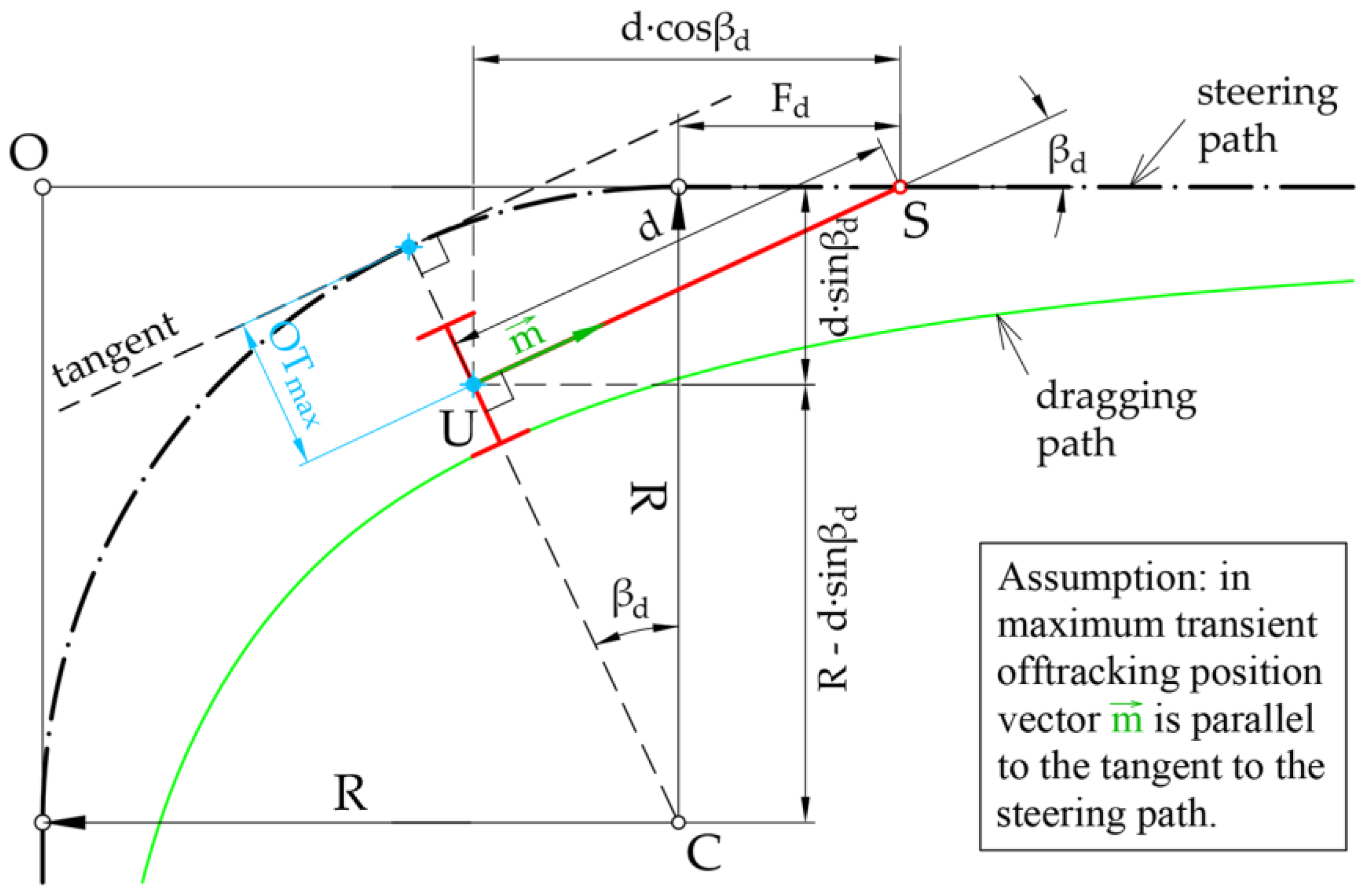
2. Problem Statement and Input Parameters
3. Mathematical Solution of the Problem
3.1. Transformation and Solving the Established Equation System
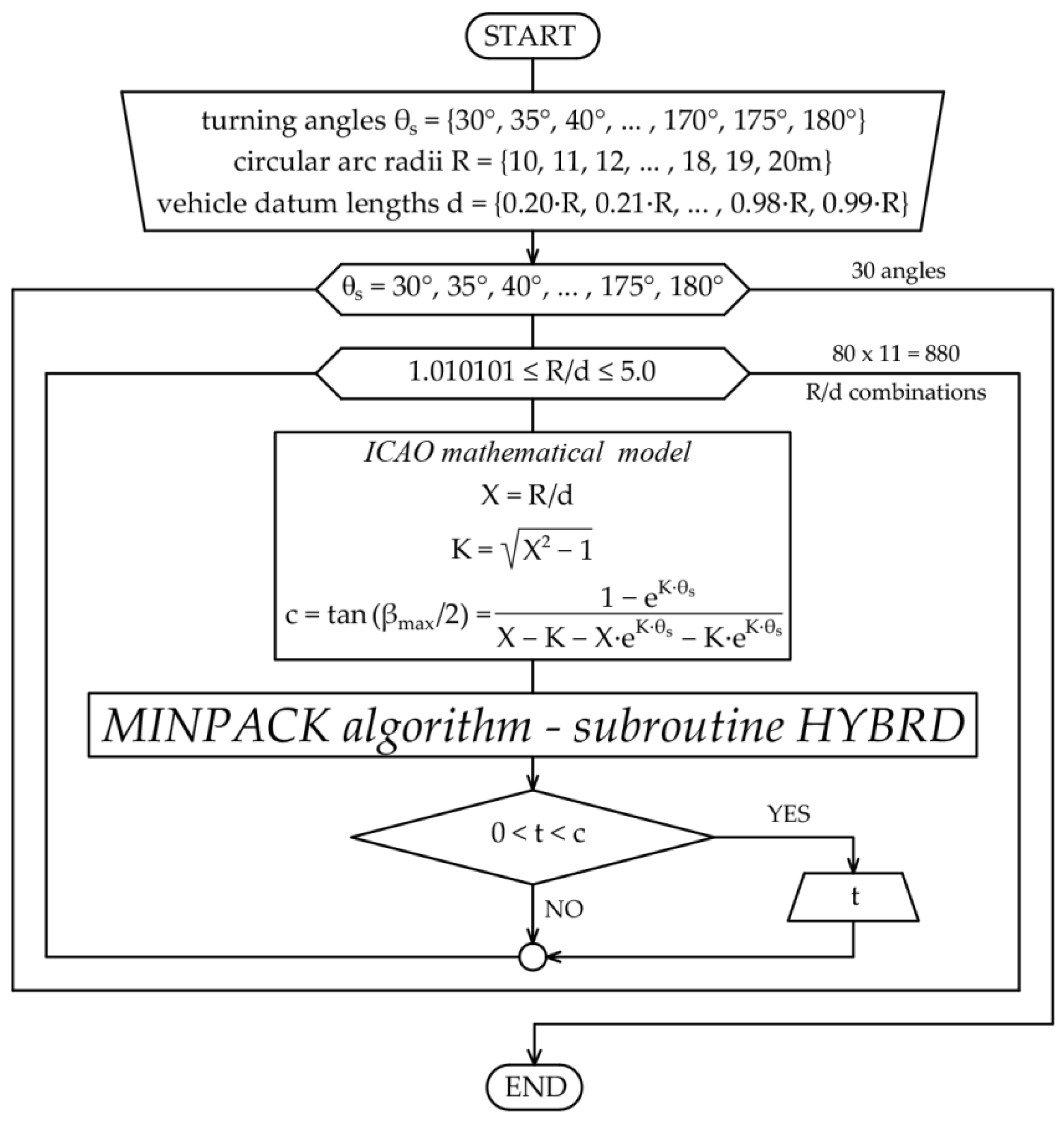
3.2. Numerical Solution of Derived Transcedental Equation
3.3. Regression Model Substituting Numerical Solution of Transcedental Equation
4. Evaluation of the Adopted Regression Model and Discussion
- Cross-validation RMSE scores: [0.00050482 0.00051121 0.00050779 0.00050810 0.00052693];
- Cross-validation mean RMSE score: 0.00051177;
- Cross-validation R2 Scores: [0.99987991 0.99988177 0.9998805 0.99987864 0.99987698];
- Cross-validation mean R2 score: 0.99987956.
- MSE on the high-value subset (HVS) range: 2.757111×10⁻⁷;
- RMSE on the HVS range: 0.000403;
- MSE on the low-value subset (LVS) range: 6.017358×10⁻⁷;
- RMSE on the LVS range: 0.000595.
5. Conclusions
Author Contributions
Funding
Institutional Review Board Statement
Informed Consent Statement
Data Availability Statement
Conflicts of Interest
Abbreviations
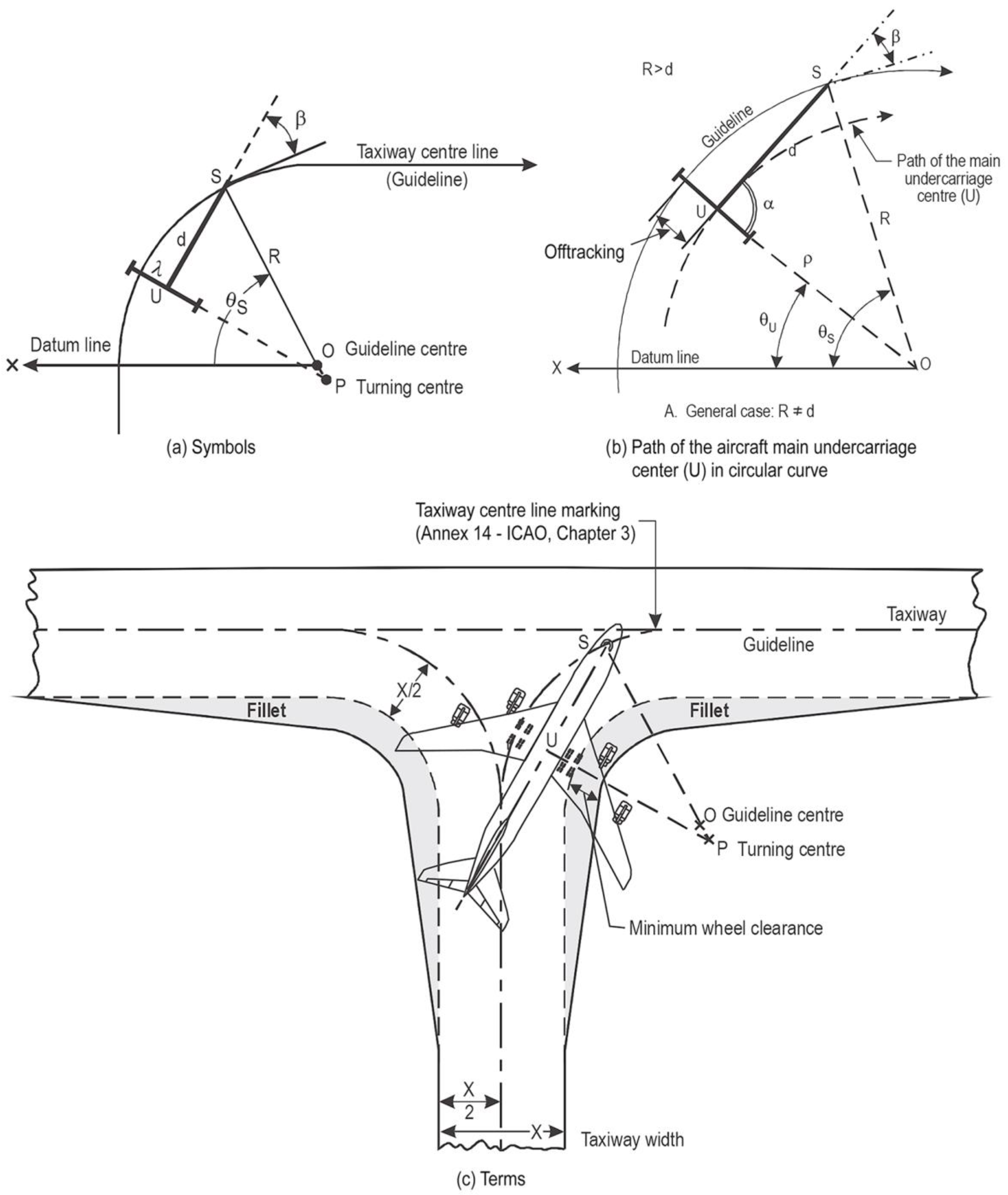
| θs | turn angle—in [°] |
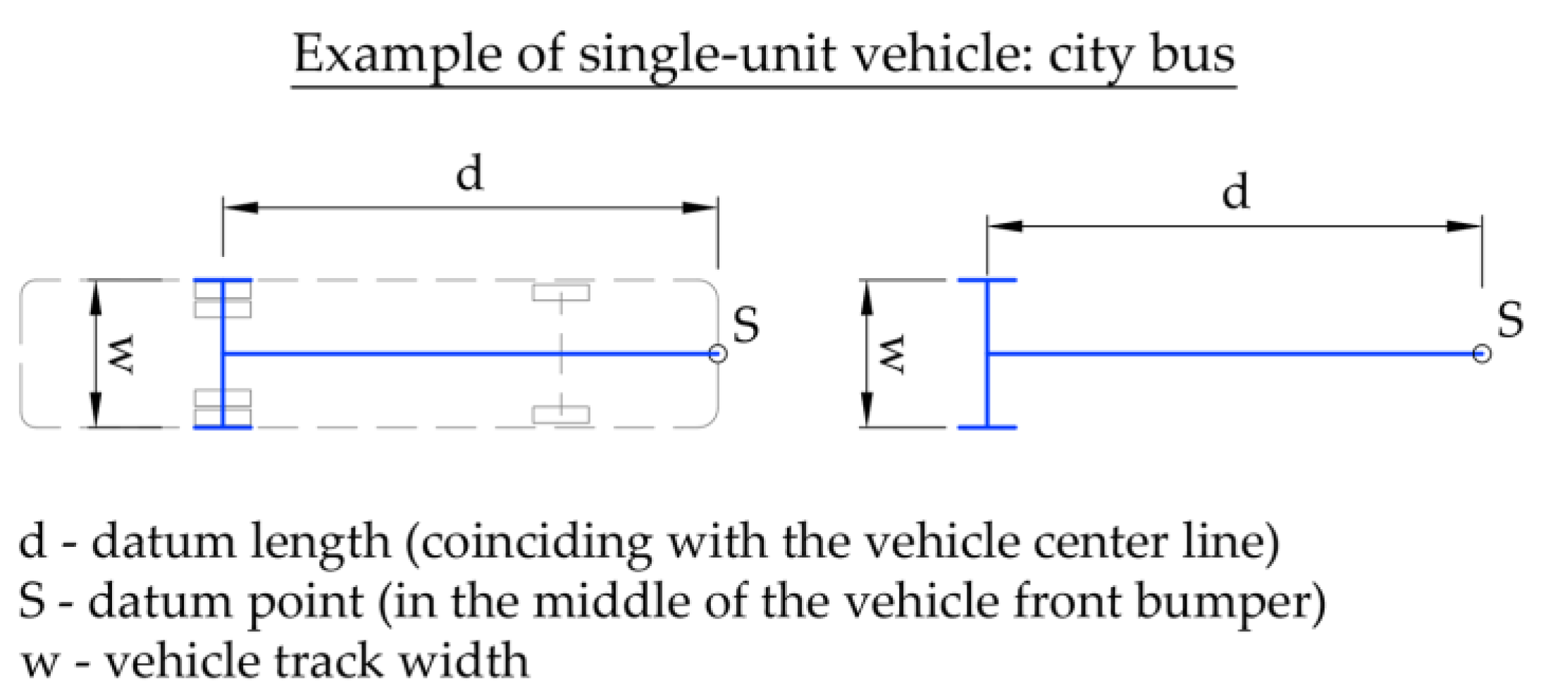
| d | aircraft (vehicle) datum length—in [m] |
| R | circular curve radii—in [m] |
| S | aircraft datum point |
| U | aircraft main undercarriage center |
| β | steering angle—in [°] |
| X | R/d ratio |
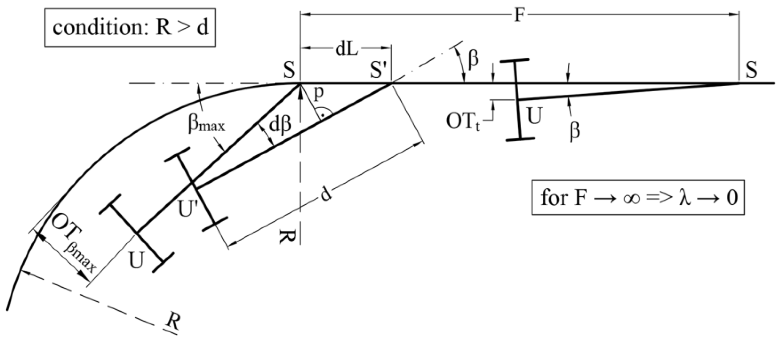
| βmax | maximum steering angle—in [°] |
| F | distance that aircraft datum point (S) covered along arc exit tangent—in [m] |
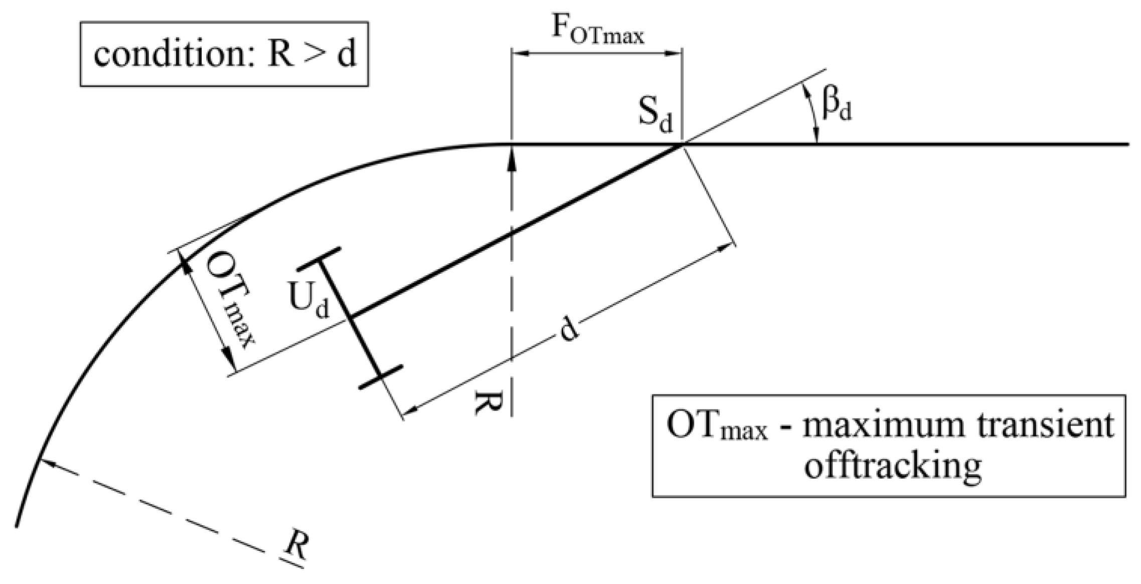
| OTmax | maximum transient offtracking—in [m] |
| FOTmax | distance that aircraft datum point (S) covered along arc exit tangent in maximum transient offtracking position—in [m] |
| w | vehicle track width—in [m] |
| βd | steering angle between the longitudinal aircraft axis and exit tangent in maximum transient offtracking position— in [°] |
| c | constant |
| t | substitution (independent variable) |
| RMSE | root mean square error |
| R2 | coefficient of determination (R-squared value) |
| MSE | mean square error |
| MDNt | median of predicted substitution t values |
| HVS | high value subset |
| LVS | low value subset |
| tN | substitution t calculated numerically |
| tR | substitution t calculated by polynomial regression function |
| βd-N | steering angle βd obtained from the substitution t numerically calculated— in [°] |
| βd-R | steering angle βd obtained from the substitution t calculated by adopted polynomial regression function— in [°] |
| FOTmax-N | distance FOTmax obtained from numerically calculated substitution t and steering angle βd-N—in [m] |
| FOTmax-R | distance FOTmax obtained from the substitution t and steering angle βd-R calculated by polynomial regression function—in [m] |
| Δβd | absolute differences between previously calculated steering angles βd-N and βd-R—in [°] |
| ΔFOTmax | absolute differences between previously calculated distances FOTmax-N and FOTmax-R—in [m] |
| OTβmax | transient offtracking calculated in the position where the maximum steering angle βmax is reached—in [m] |
References
- AASHTO. Elements of design—Horizontal alignment. In The Green Book—A Policy on Geometric Design of Highways and Streets, 7th ed.; American Association of State Highway and Transportation Officials—AASHTO: Washington, DC, USA, 2018; pp. 90–96. [Google Scholar]
- Jindra, F. Off-Tracking of Tractor-Trailer Combinations. In Automobile Engineer; SAE International: London, UK, 1963; pp. 96–101. [Google Scholar]
- Sayers, M.W. Vehicle Offtracking Models; Transportation Research Record 1052; Transportation Research Board: Washington, DC, USA, 1986; pp. 53–62. [Google Scholar]
- Choi, J.; Lee, S.; Baek, J.; Kang, W. Offtracking Model on Horizontal Curve Sections. Proc. East. Asia Soc. Transp. Stud. 2001, 3, 341–353. [Google Scholar]
- National Academies of Sciences, Engineering, and Medicine. NCHRP Report 505: Review of Truck Characteristics as Factors in Roadway Design; The National Academies Press: Washington, DC, USA, 2003; pp. 39–44. [Google Scholar] [CrossRef]
- Erkert, T.W.; Sessions, J.; Layton, R.D. A Method for Determining Offtracking of Multiple Unit Vehicle Combinations. J. For. Eng. 1989, 1, 9–16. [Google Scholar] [CrossRef]
- Woodrooffe, J.H.F.; Smith, C.A.M.; Morisset, L.E. A Generalized Solution of Non-Steady State Vehicle Off Tracking in Constant Radius Curves. In Proceedings of the 3rd International Pacific Conference on Automotive Engineering: Motor Vehicle Technology: Mobility for prosperity, Jakarta, Indonesia, 11–14 November 1985. [Google Scholar] [CrossRef]
- WHI. Offtracking Characteristics of Trucks and Truck Combinations; Research Committee Report No. 3; Western Highway Institute: San Bruno, CA, USA, 1970; pp. 7–45. [Google Scholar]
- SAE. Turning Ability and Off Tracking—Motor Vehicles; SAE Recommended Practice, J695_201106; Society of Automobile Engineers—SAE International: Warrendale, PA, USA, 2011; p. 13. [Google Scholar] [CrossRef]
- SAE. Turning Ability and Off Tracking—Motor Vehicles; SAE Recommended Practice, J695_202401; Society of Automobile Engineers—SAE International: Warrendale, PA, USA, 2024; p. 12. [Google Scholar] [CrossRef]
- ICAO. Appendix 1—Fillet design. In Aerodrome Design Manual—Part 2: Taxiways, Aprons and Holding Bays, 5th ed.; International Civil Aviation Organization: Montreal, QC, Canada, 2020; pp. 97–143. [Google Scholar]
- Yao, Q.; Tian, Y.; Wang, Q.; Wang, S. Control Strategies on Path Tracking for Autonomous Vehicle: State of the Art and Future Challenges. IEEE Access 2020, 8, 161211–161222. [Google Scholar] [CrossRef]
- Othman, K. Impact of Autonomous Vehicles on the Physical Infrastructure: Changes and Challenges. Designs 2021, 5, 40. [Google Scholar] [CrossRef]
- Kebbati, Y.; Ait-Oufroukh, N.; Ichalal, D.; Vigneron, V. Lateral control for autonomous wheeled vehicles: A technical review. Asian J. Control 2023, 25, 2539–2563. [Google Scholar] [CrossRef]
- Jawahar, A.; Palla, L. Lateral Control of Heavy Vehicles. Master’s Thesis, KTH Royal Institute of Technology, School of Engineering Sciences, Stockholm, Sweden, 2023. [Google Scholar]
- Shaju, A.; Southward, S.; Ahmadian, M. Enhancing Autonomous Vehicle Navigation with a Clothoid-Based Lateral Controller. Appl. Sci. 2024, 14, 1817. [Google Scholar] [CrossRef]
- Sayers, M.W. Symbolic Computer Methods to Automatically Formulate Vehicle Simulation Codes. Doctoral Thesis, The University of Michigan Transportation Research Institute, Ann Arbor, MI, USA, 1990. [Google Scholar]
- Sayers, M.W. Exact Equations for Tractrix Curves Associated with Vehicle Offtracking. Veh. Syst. Dyn. 1991, 20, 297–308. [Google Scholar] [CrossRef]
- Garlick, G.S.; Kanga, D.N.; Miller, G.G. Vehicle Offtracking: A Globally Stable Solution. ITE J. 1993, 63, 17–21. [Google Scholar]
- Wang, Y.; Linnett, J.A. Vehicle Kinematics and Its Application to Highway Design. J. Transp. Eng.-ASCE 1995, 121, 63–74. [Google Scholar] [CrossRef]
- Dragčević, V. Numerical Model of Motion of Road Vehicles. Doctoral Thesis, The University of Zagreb, Faculty of Civil Engineering, Zagreb, Croatia, 1999. [Google Scholar]
- Prince, G.E.; Dubois, S.P. Mathematical Models for Motion of the Rear Ends of Vehicles. Math. Comput. Model. 2009, 49, 2049–2060. [Google Scholar] [CrossRef]
- Cheng, J.F.; Huang, H.C. Effects of Roadway Geometric Features on Low- Speed Turning Maneuvers of Large Vehicles. Int. J. Pavement Res. Technol. 2011, 4, 373–383. [Google Scholar]
- Autodesk. Vehicle Tracking: Swept Path Analysis and Design Software. Available online: https://www.autodesk.com/products/vehicle-tracking/overview (accessed on 11 April 2024).
- Transoft Solutions. AutoTURN: Vehicle Simulation Software. Available online: https://www.transoftsolutions.com/emea/civil-and-transportation/software/swept-path-analysis/autoturn/ (accessed on 11 April 2024).
- Ilić, V. Analytical Method for Critical Vehicle Swept Path Testing and Intersection Layout Elements Calculation. Doctoral Thesis, The University of Belgrade, Faculty of Civil Engineering, Belgrade, Serbia, 2019. [Google Scholar]
- Lawrence, G.J. A mathematical Model for the Low-Speed Offtracking of Articulated Vehicles That Includes Tire Mechanics. Master’s Thesis, The University of Calgary, Department of Mechanical Engineering, Calgary, AB, Canada, 1987. [Google Scholar]
- Dragčević, V.; Korlaet, Ž.; Stančerić, I. Methods for Setting Road Vehicle Movements Trajectories. Balt. J. Road Bridge Eng. 2008, 3, 57–64. [Google Scholar] [CrossRef]
- Stančerić, I.; Korlaet, Ž.; Dragčević, V. New design procedure for four-leg channelized intersections. Građevinar 2017, 69, 257–266. [Google Scholar] [CrossRef]
- Forschungsgessellschaft für Straßen und Verkehrswesen (FGSV). Richtlinien für die Anlage von Landstrassen—RAL, Abschnitt 6: Knotenpunkte, Unterabschnitt 6.4: Knotenpunktelemente—Rechtsabbiegen; Forschungsgessellschaft für Straßen und Verkehrswesen (FGSV): Köln, Germany, 2012. [Google Scholar]
- CGS Labs. Autopath: Swept Path Analysis and Vehicle Turning Simulation Software. Available online: https://cgs-labs.com/autopath/ (accessed on 13 April 2024).
- Luck, R.; Zdaniuk, G.J.; Cho, H. An Efficient Method to Find Solutions for Transcendental Equations with Several Roots. Int. J. Eng. Math. 2015, 2015, 523043. [Google Scholar] [CrossRef]
- HYBRD. Documentation for MINPACK Subroutine HYBRD. Available online: https://www.math.utah.edu/software/minpack/minpack/hybrd.html (accessed on 26 April 2024).
- Real Python. Advanced Python Tutorials. Available online: https://realpython.com/tutorials/advanced/ (accessed on 30 April 2024).


| Input Parameters | Results | ||||||||||
|---|---|---|---|---|---|---|---|---|---|---|---|
| No * | θS [°] | R [m] | d [m] | R/d | K | eKθs | c | βmax [°] | t | βd [°] | |
| 1 | 30.00 | 10.00 | 2.00 | 5.000000 | 4.898979 | 13.001954 | 0.093324 | 10.6633 | 0.066106 | 7.5642 | |
| 2 | 30.00 | 10.00 | 2.10 | 4.761905 | 4.655721 | 11.447024 | 0.097003 | 11.0811 | 0.067365 | 7.7078 | |
| 3 | 30.00 | 10.00 | 2.20 | 4.545455 | 4.434090 | 10.192827 | 0.100561 | 11.4848 | 0.068529 | 7.8406 | |
| 4 | 30.00 | 10.00 | 2.30 | 4.347826 | 4.231264 | 9.165848 | 0.104000 | 11.8748 | 0.069609 | 7.9637 | |
| 5 | 30.00 | 10.00 | 2.40 | 4.166667 | 4.044887 | 8.313643 | 0.107323 | 12.2514 | 0.070612 | 8.0782 | |
| 6 | 30.00 | 10.00 | 2.50 | 4.000000 | 3.872983 | 7.598033 | 0.110534 | 12.6151 | 0.071547 | 8.1848 | |
| 7 | 30.00 | 10.00 | 2.60 | 3.846154 | 3.713879 | 6.990714 | 0.113638 | 12.9663 | 0.072420 | 8.2843 | |
| 8 | 30.00 | 10.00 | 2.70 | 3.703704 | 3.566149 | 6.470358 | 0.116636 | 13.3054 | 0.073236 | 8.3773 | |
| 9 | 30.00 | 10.00 | 2.80 | 3.571429 | 3.428571 | 6.020653 | 0.119534 | 13.6330 | 0.074001 | 8.4645 | |
| 10 | 30.00 | 10.00 | 2.90 | 3.448276 | 3.300092 | 5.628956 | 0.122336 | 13.9493 | 0.074720 | 8.5464 | |
| 11 | 30.00 | 10.00 | 3.00 | 3.333333 | 3.179797 | 5.285346 | 0.125044 | 14.2550 | 0.075395 | 8.6233 | |
| 12 | 30.00 | 10.00 | 3.10 | 3.225806 | 3.066892 | 4.981948 | 0.127663 | 14.5504 | 0.076031 | 8.6958 | |
| 13 | 30.00 | 10.00 | 3.20 | 3.125000 | 2.960680 | 4.712452 | 0.130197 | 14.8360 | 0.076632 | 8.7642 | |
| 14 | 30.00 | 10.00 | 3.30 | 3.030303 | 2.860548 | 4.471749 | 0.132648 | 15.1121 | 0.077199 | 8.8288 | |
| 15 | 30.00 | 10.00 | 3.40 | 2.941176 | 2.765957 | 4.255668 | 0.135020 | 15.3792 | 0.077736 | 8.8900 | |
| 16 | 30.00 | 10.00 | 3.50 | 2.857143 | 2.676428 | 4.060777 | 0.137317 | 15.6376 | 0.078244 | 8.9479 | |
| 17 | 30.00 | 10.00 | 3.60 | 2.777778 | 2.591534 | 3.884227 | 0.139541 | 15.8876 | 0.078727 | 9.0029 | |
| • | • | • | • | • | • | • | • | • | • | • | |
| • | • | • | • | • | • | • | • | • | • | • | |
| • | • | • | • | • | • | • | • | • | • | • | |
| 26,384 | 180.00 | 20.00 | 16.60 | 1.204819 | 0.672004 | 8.257840 | 0.484965 | 51.7435 | 0.357094 | 39.3026 | |
| 26,385 | 180.00 | 20.00 | 16.80 | 1.190476 | 0.645936 | 7.608518 | 0.492151 | 52.4083 | 0.359695 | 39.5668 | |
| 26,386 | 180.00 | 20.00 | 17.00 | 1.176471 | 0.619744 | 7.007523 | 0.499366 | 53.0720 | 0.362259 | 39.8268 | |
| 26,387 | 180.00 | 20.00 | 17.20 | 1.162791 | 0.593365 | 6.450203 | 0.506612 | 53.7347 | 0.364787 | 40.0826 | |
| 26,388 | 180.00 | 20.00 | 17.40 | 1.149425 | 0.566726 | 5.932363 | 0.513888 | 54.3961 | 0.367279 | 40.3345 | |
| 26,389 | 180.00 | 20.00 | 17.60 | 1.136364 | 0.539743 | 5.450199 | 0.521193 | 55.0564 | 0.369736 | 40.5823 | |
| 26,390 | 180.00 | 20.00 | 17.80 | 1.123596 | 0.512315 | 5.000239 | 0.528526 | 55.7153 | 0.372158 | 40.8263 | |
| 26,391 | 180.00 | 20.00 | 18.00 | 1.111111 | 0.484322 | 4.579285 | 0.535889 | 56.3727 | 0.374546 | 41.0665 | |
| 26,392 | 180.00 | 20.00 | 18.20 | 1.098901 | 0.455613 | 4.184352 | 0.543280 | 57.0287 | 0.376901 | 41.3030 | |
| 26,393 | 180.00 | 20.00 | 18.40 | 1.086957 | 0.425998 | 3.812606 | 0.550699 | 57.6830 | 0.379224 | 41.5358 | |
| 26,394 | 180.00 | 20.00 | 18.60 | 1.075269 | 0.395225 | 3.461274 | 0.558145 | 58.3357 | 0.381514 | 41.7651 | |
| 26,395 | 180.00 | 20.00 | 18.80 | 1.063830 | 0.362952 | 3.127537 | 0.565619 | 58.9866 | 0.383773 | 41.9909 | |
| 26,396 | 180.00 | 20.00 | 19.00 | 1.052632 | 0.328684 | 2.808334 | 0.573119 | 59.6357 | 0.386001 | 42.2132 | |
| 26,397 | 180.00 | 20.00 | 19.20 | 1.041667 | 0.291667 | 2.500018 | 0.580647 | 60.2829 | 0.388198 | 42.4322 | |
| 26,398 | 180.00 | 20.00 | 19.40 | 1.030928 | 0.250624 | 2.197581 | 0.588200 | 60.9281 | 0.390366 | 42.6480 | |
| 26,399 | 180.00 | 20.00 | 19.60 | 1.020408 | 0.203059 | 1.892555 | 0.595780 | 61.5713 | 0.392505 | 42.8605 | |
| 26,400 | 180.00 | 20.00 | 19.80 | 1.010101 | 0.142492 | 1.564635 | 0.603385 | 62.2123 | 0.394615 | 43.0699 | |
| Nonlinear Regression Model Type | RMSE |
|---|---|
| Polynomial Regression (4th degree) | 0.000496 |
| Ridge Regression | 0.002261 |
| Lasso Regression | 0.073637 |
| Elastic Net Regression | 0.073637 |
| Decision Tree Regression | 0.002843 |
| Random Forest Regression | 0.000995 |
| Support Vector Regression—SVR | 0.051933 |
| Gradient Boosting Regression | 0.001854 |
| K Neighbors Regression | 0.001480 |
| AdaBoost Regression | 0.009943 |
| Degree of Polynomial Regression Model | Lateral Positioning Error [m] | RMSE | R2 |
|---|---|---|---|
| 2nd-degree polynomial regression | >0.100 | 0.002453 | 0.99904 |
| 3rd-degree polynomial regression | 0.050 | 0.001754 | 0.99944 |
| 4th-degree polynomial regression | 0.025 | 0.000496 | 0.99988 |
| No | Methods | Brief Description of Steps to Test the Robustness of the Selected Method |
|---|---|---|
| 1 | K-Fold Cross-Validation | The procedure has a single parameter called k that refers to the number of groups that a given data sample is to be split into. As such, the procedure is often called k-fold cross-validation. |
| 2 | Repeated Train/Test Splits | Perform multiple train/test splits with different random seeds and evaluate the model on each split. Calculate and compare the performance metrics (e.g., R2, RMSE) across these splits. |
| 3 | Robustness to Noise | Add different levels of noise to the input features and observe changes in performance metrics. For example, Gaussian noise can be added to analyzed features to see how the model’s predictions and accuracy are affected. |
| 4 | Outlier Analysis | Introduce synthetic outliers into the dataset and evaluate the model’s robustness by observing changes in performance metrics. |
| 5 | Generalization to Unseen Data | If researchers have access to an external dataset that was not used in training, they can evaluate the model on this dataset to check its generalization capabilities. |
| 6 | Stress Testing with Extreme Values | Test the regression model with extreme or edge-case values for input features to evaluate how it handles these unusual cases. |
| Input Parameters | Numerical Solution | Regression Model | Abs. Differences | |||||||||||
|---|---|---|---|---|---|---|---|---|---|---|---|---|---|---|
| No * | θS [°] | R/d | βmax [°] | tN | βd-N [°] | FOTmax-N | tR | βd-R [°] | FOTmax- R [m] | Δβd [°] | ΔFOTmax [m] | |||
| 1 | 30.00 | 5.000000 | 10.6633 | 0.066106 | 7.5642 | 0.690 | 0.073171 | 8.3699 | 0.487 | 0.8057 | 0.203 | |||
| 2 | 30.00 | 4.761905 | 11.0811 | 0.067365 | 7.7078 | 0.766 | 0.072593 | 8.3039 | 0.609 | 0.5962 | 0.157 | |||
| 3 | 30.00 | 4.545455 | 11.4848 | 0.068529 | 7.8406 | 0.844 | 0.070955 | 8.1172 | 0.767 | 0.2767 | 0.077 | |||
| 4 | 30.00 | 4.347826 | 11.8748 | 0.069609 | 7.9637 | 0.923 | 0.070269 | 8.0390 | 0.902 | 0.0753 | 0.022 | |||
| 5 | 30.00 | 4.166667 | 12.2514 | 0.070612 | 8.0782 | 1.005 | 0.070210 | 8.0323 | 1.018 | 0.0459 | 0.014 | |||
| 6 | 30.00 | 4.000000 | 12.6151 | 0.071547 | 8.1848 | 1.087 | 0.070559 | 8.0721 | 1.122 | 0.1127 | 0.035 | |||
| 7 | 30.00 | 3.846154 | 12.9663 | 0.072420 | 8.2843 | 1.171 | 0.071166 | 8.1413 | 1.217 | 0.1430 | 0.045 | |||
| 8 | 30.00 | 3.703704 | 13.3054 | 0.073236 | 8.3773 | 1.256 | 0.071928 | 8.2282 | 1.305 | 0.1491 | 0.049 | |||
| 9 | 30.00 | 3.571429 | 13.6330 | 0.074001 | 8.4645 | 1.343 | 0.072777 | 8.3249 | 1.389 | 0.1396 | 0.047 | |||
| 10 | 30.00 | 3.448276 | 13.9493 | 0.074720 | 8.5464 | 1.430 | 0.073663 | 8.4260 | 1.471 | 0.1204 | 0.041 | |||
| 11 | 30.00 | 3.333333 | 14.2550 | 0.075395 | 8.6233 | 1.518 | 0.074557 | 8.5278 | 1.551 | 0.0955 | 0.034 | |||
| 12 | 30.00 | 3.225806 | 14.5504 | 0.076031 | 8.6958 | 1.607 | 0.075436 | 8.6280 | 1.631 | 0.0678 | 0.024 | |||
| 13 | 30.00 | 3.125000 | 14.8360 | 0.076632 | 8.7642 | 1.696 | 0.076287 | 8.7249 | 1.711 | 0.0393 | 0.014 | |||
| 14 | 30.00 | 3.030303 | 15.1121 | 0.077199 | 8.8288 | 1.786 | 0.077100 | 8.8176 | 1.791 | 0.0112 | 0.004 | |||
| 15 | 30.00 | 2.941176 | 15.3792 | 0.077736 | 8.8900 | 1.877 | 0.077872 | 8.9055 | 1.871 | 0.0156 | 0.006 | |||
| 16 | 30.00 | 2.857143 | 15.6376 | 0.078244 | 8.9479 | 1.969 | 0.078600 | 8.9884 | 1.953 | 0.0405 | 0.016 | |||
| 17 | 30.00 | 2.777778 | 15.8876 | 0.078727 | 9.0029 | 2.061 | 0.079283 | 9.0662 | 2.035 | 0.0633 | 0.025 | |||
| • | • | • | • | • | • | • | • | • | • | • | • | |||
| • | • | • | • | • | • | • | • | • | • | • | • | |||
| • | • | • | • | • | • | • | • | • | • | • | • | |||
| 26,383 | 180.00 | 1.219512 | 51.0779 | 0.354454 | 39.0342 | 4.898 | 0.354516 | 39.0405 | 4.895 | 0.0063 | 0.003 | |||
| 26,384 | 180.00 | 1.204819 | 51.7435 | 0.357094 | 39.3026 | 5.081 | 0.357041 | 39.2973 | 5.083 | 0.0053 | 0.002 | |||
| 26,385 | 180.00 | 1.190476 | 52.4083 | 0.359695 | 39.5668 | 5.267 | 0.359525 | 39.5496 | 5.275 | 0.0172 | 0.008 | |||
| 26,386 | 180.00 | 1.176471 | 53.0720 | 0.362259 | 39.8268 | 5.457 | 0.361969 | 39.7974 | 5.470 | 0.0294 | 0.014 | |||
| 26,387 | 180.00 | 1.162791 | 53.7347 | 0.364787 | 40.0826 | 5.649 | 0.364375 | 40.0409 | 5.668 | 0.0417 | 0.019 | |||
| 26,388 | 180.00 | 1.149425 | 54.3961 | 0.367279 | 40.3345 | 5.844 | 0.366742 | 40.2802 | 5.870 | 0.0543 | 0.025 | |||
| 26,389 | 180.00 | 1.136364 | 55.0564 | 0.369736 | 40.5823 | 6.043 | 0.369071 | 40.5153 | 6.074 | 0.0670 | 0.032 | |||
| 26,390 | 180.00 | 1.123596 | 55.7153 | 0.372158 | 40.8263 | 6.244 | 0.371364 | 40.7464 | 6.282 | 0.0799 | 0.038 | |||
| 26,391 | 180.00 | 1.111111 | 56.3727 | 0.374546 | 41.0665 | 6.448 | 0.373621 | 40.9735 | 6.492 | 0.0930 | 0.045 | |||
| 26,392 | 180.00 | 1.098901 | 57.0287 | 0.376901 | 41.3030 | 6.655 | 0.375843 | 41.1968 | 6.706 | 0.1062 | 0.051 | |||
| 26,393 | 180.00 | 1.086957 | 57.6830 | 0.379224 | 41.5358 | 6.864 | 0.378030 | 41.4162 | 6.922 | 0.1196 | 0.058 | |||
| 26,394 | 180.00 | 1.075269 | 58.3357 | 0.381514 | 41.7651 | 7.077 | 0.380184 | 41.6320 | 7.142 | 0.1331 | 0.065 | |||
| 26,395 | 180.00 | 1.063830 | 58.9866 | 0.383773 | 41.9909 | 7.292 | 0.382305 | 41.8442 | 7.364 | 0.1466 | 0.072 | |||
| 26,396 | 180.00 | 1.052632 | 59.6357 | 0.386001 | 42.2132 | 7.510 | 0.384394 | 42.0529 | 7.589 | 0.1603 | 0.079 | |||
| 26,397 | 180.00 | 1.041667 | 60.2829 | 0.388198 | 42.4322 | 7.730 | 0.386451 | 42.2581 | 7.817 | 0.1741 | 0.087 | |||
| 26,398 | 180.00 | 1.030928 | 60.9281 | 0.390366 | 42.6480 | 7.954 | 0.388477 | 42.4600 | 8.048 | 0.1880 | 0.094 | |||
| 26,399 | 180.00 | 1.020408 | 61.5713 | 0.392505 | 42.8605 | 8.180 | 0.390473 | 42.6586 | 8.281 | 0.2019 | 0.102 | |||
| 26,400 | 180.00 | 1.010101 | 62.2123 | 0.394615 | 43.0699 | 8.408 | 0.392439 | 42.8540 | 8.517 | 0.2159 | 0.109 | |||
Disclaimer/Publisher’s Note: The statements, opinions and data contained in all publications are solely those of the individual author(s) and contributor(s) and not of MDPI and/or the editor(s). MDPI and/or the editor(s) disclaim responsibility for any injury to people or property resulting from any ideas, methods, instructions or products referred to in the content. |
© 2024 by the authors. Licensee MDPI, Basel, Switzerland. This article is an open access article distributed under the terms and conditions of the Creative Commons Attribution (CC BY) license (https://creativecommons.org/licenses/by/4.0/).
Share and Cite
Ilić, V.; Lukić, M.; Gavran, D.; Fric, S.; Trpčevski, F.; Vranjevac, S.; Milovanović, N. Exact Mathematical Solution for Maximum Transient Offtracking Calculation of a Single-Unit Vehicle Negotiating Circular Curves. Appl. Sci. 2024, 14, 5570. https://doi.org/10.3390/app14135570
Ilić V, Lukić M, Gavran D, Fric S, Trpčevski F, Vranjevac S, Milovanović N. Exact Mathematical Solution for Maximum Transient Offtracking Calculation of a Single-Unit Vehicle Negotiating Circular Curves. Applied Sciences. 2024; 14(13):5570. https://doi.org/10.3390/app14135570
Chicago/Turabian StyleIlić, Vladan, Miloš Lukić, Dejan Gavran, Sanja Fric, Filip Trpčevski, Stefan Vranjevac, and Nikola Milovanović. 2024. "Exact Mathematical Solution for Maximum Transient Offtracking Calculation of a Single-Unit Vehicle Negotiating Circular Curves" Applied Sciences 14, no. 13: 5570. https://doi.org/10.3390/app14135570
APA StyleIlić, V., Lukić, M., Gavran, D., Fric, S., Trpčevski, F., Vranjevac, S., & Milovanović, N. (2024). Exact Mathematical Solution for Maximum Transient Offtracking Calculation of a Single-Unit Vehicle Negotiating Circular Curves. Applied Sciences, 14(13), 5570. https://doi.org/10.3390/app14135570