1. Introduction
The cooperative initiative of establishing the Belt and Road was proposed by Xi Jinping, President of the People’s Republic of China, in Kazakhstan and Indonesia in 2013, respectively, which aims to establish the world’s biggest economic cooperation platform covering Asia, Europe, and sub-regions of Africa and enhance the interconnectivity among countries. Currently, China Railway Express (CR Express), with active participation from local governments, has connected 108 Chinese cities and reached 208 cities in 25 European countries through ports such as Manzhouli, Erenhot, and Alashankou [
1]. Meanwhile, as of September 2022, there are 94 routes along Maritime Silk Road, connecting 108 ports in 31 countries [
2]. The in-depth development of the transportation network has greatly shortened the time and space distance between China and Europe. Currently, the Chinese local governments are faced with various issues in the process of promoting the in-depth development of the BRI, such as uneven supplies of goods, disordered competition, and inefficient coordination mechanism [
3,
4]. On the other hand, the Chinese domestic transportation network is a relatively independent development of various transportation modes, which lacks global optimization and integration of transportation resources. To address the above-mentioned issues, constructing consolidation centers through top-level government design is a promising solution to provide rational cargo allocation. This is because the rational location and layout of the consolidation centers can reduce logistics costs through economies of scale, as well as maximize service quality and transportation efficiency within multimodal networks [
5,
6].
Therefore, the issue of transportation hubs along the Belt and Road has been discussed by many scholars from different perspectives in the past few years. Zhang et al. applied the TOPSIS to sort out the logistics nodes and select the optimal nodes of CR Express under the BRI [
7]. Li et al. applied contest theory to validate the number of multimodal transportation network hubs based on local government subsidies under the BRI [
8]. Wan et al. used the TOPSIS to identify essential ports in the maritime silk network when encountering severe disasters [
9]. By analyzing the quantitative and qualitative factors influencing the location of global logistics centers in the existing literature, Lee et al. proposed the eight locations of global LDCs [
10]. Li et al. considered the government policies and operational experience from the BRI, and used the improved entropy TOPSIS to select imported grain distribution centers across railway, highway, and water transportation networks [
11]. The TOPSIS was employed by Aljohani et al. to conduct an assessment and ranking of 20 candidate consolidation centers within the city of inner Melbourne, Australia, based on 11 decision criteria, and found that the most suitable locations for the consolidation centers are in economically viable industrial areas [
12]. Muerza et al. used ANP technology to evaluate and rank five locations in Europe for establishing international consolidation centers based on 25 standards to support the choices of decision makers [
13].
Furthermore, during a meeting with the leader of Luxembourg in June 2017, President Xi Jinping first proposed to build the Air Silk Road between Zhengzhou and Luxembourg. With the gradual integration of the civil aviation industry into the BRI, the Chinese government released an Implementation Plan of the Air Silk Road in May 2022, aiming to promote its in-depth development [
14]. Meanwhile, scholars have begun to address the issues of the air transportation network. Zhou et al. employed local centrality and global centrality to research the hub problem of the integration of rail ports, airports, and maritime ports in the Belt and Road countries [
15]. Derudder et al. applied the centrality indicator to study the ranking of connectivity of three-layer transportation network node cities for air and highway routes along the Belt and Road [
16].
However, the above-mentioned scholars are only concerned about a single mode or a combination of two or three transport modes, and there is less research on the integration of railway, air, highway, and water transportation. Additionally, the whole layout of the integrated transportation network has not been formed at the national level, which cannot effectively fit in with the development of the BRI, making it difficult to effectively achieve the orderly linking up of the multi-tiered integrated transportation network consisting of water, land, and air transportation. Hence, this paper addresses the ranking and selection of node cities as the candidate consolidation centers of an integrated transportation network composed of highway, railway, air, and water routes under the BRI to provide a reference for the government in building the consolidation centers.
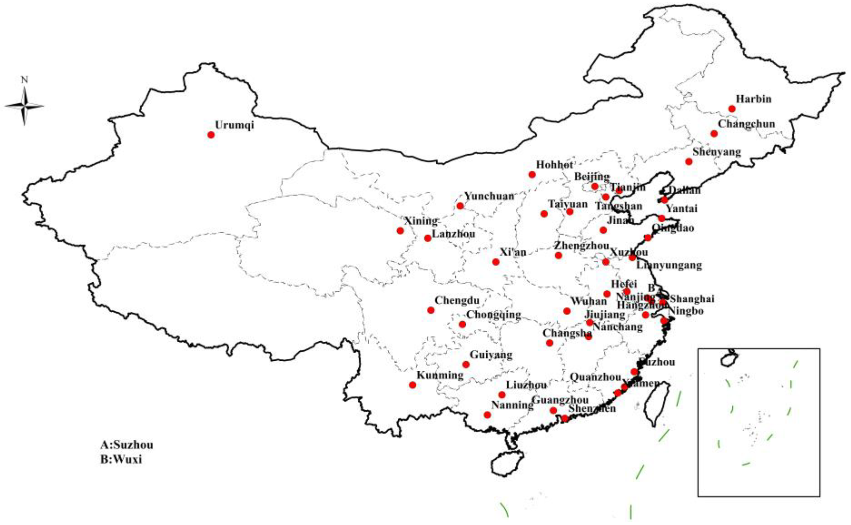
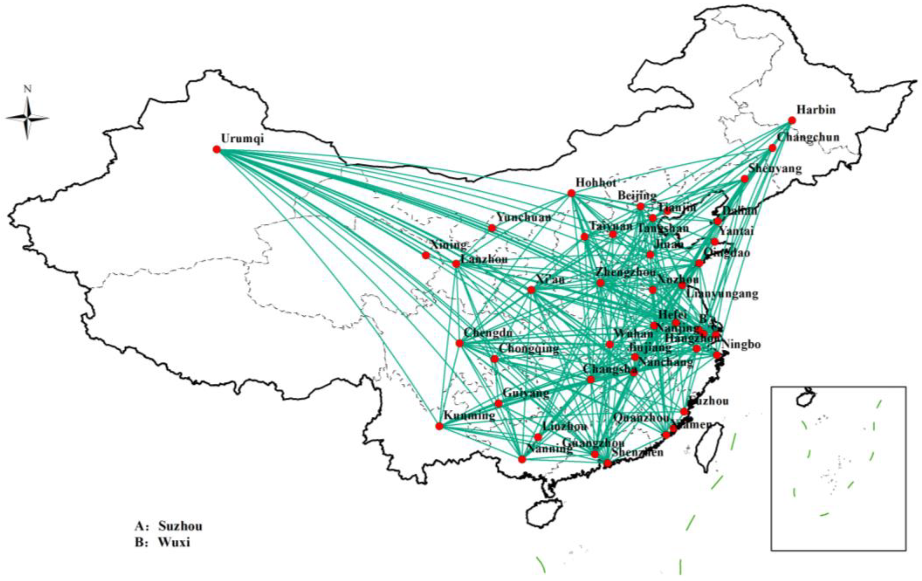
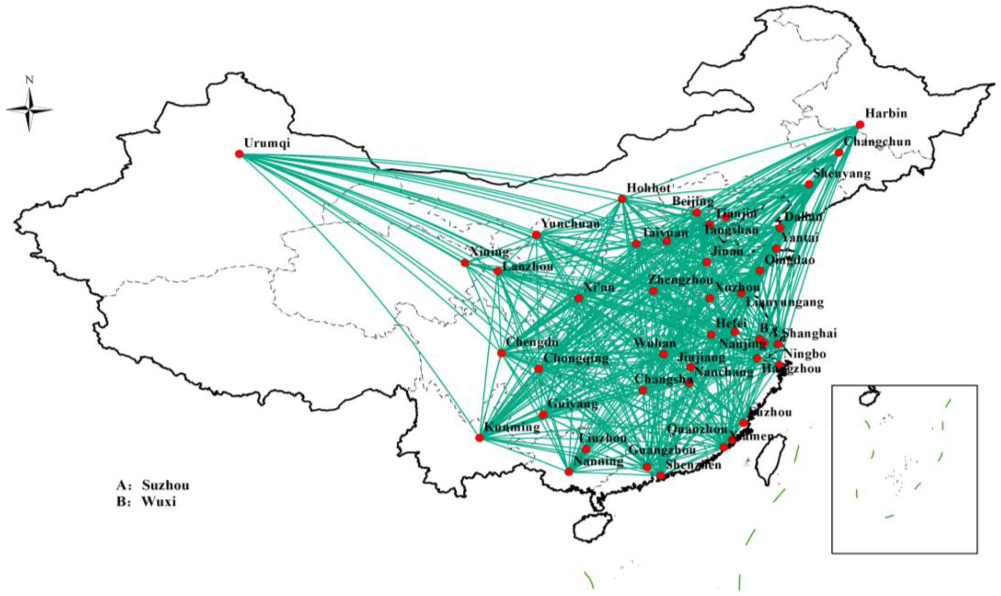
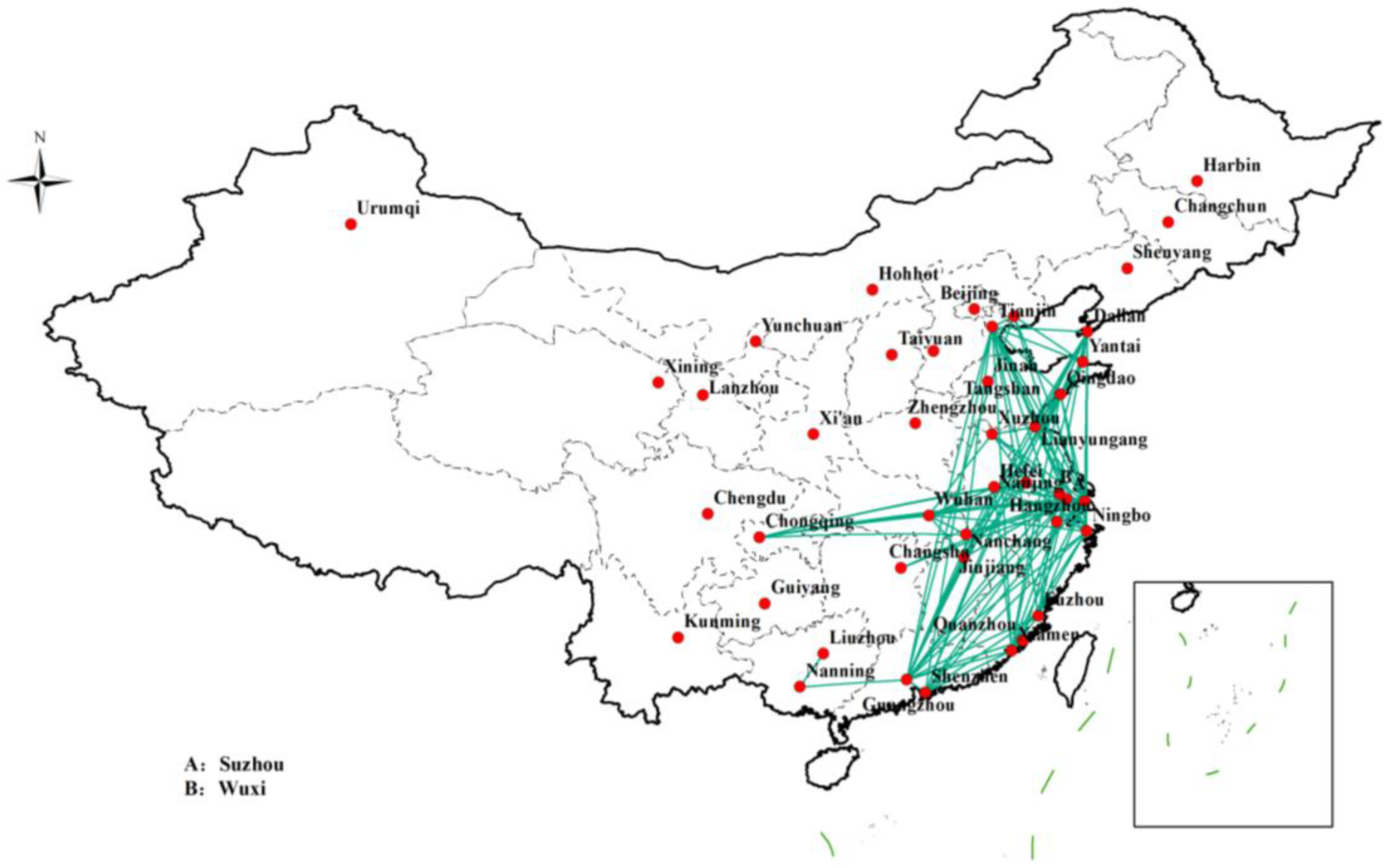
A total of 44 Chinese cities were selected as the candidate consolidation centers under the BRI. Then, the integrated transportation network was formed based on the links of transportation modes among these 44 Chinese cities. It should be noted that the evaluation of consolidation centers in this study was based on the consideration of the above issues of cargo transportation at the national level of China under the BRI. Consequently, each city was viewed as a node in the network without delving into the specific logistic activities within it.
Complex network theory has been widely employed in transportation network research in recent years [
17,
18]; extensive study has been implemented on single-mode transportation networks, including railway networks [
11], subway networks [
19,
20], bus networks [
21,
22], water networks [
23,
24], road networks [
25], and air networks [
26]. Currently, complex network theory is employed by some scholars to study the single-mode transportation networks under the BRI. Zhao et al. used the TOPSIS method combined with complex network theory to select 10 cities from 27 candidate cities as consolidation centers of CR Express [
27]. Sun et al. applied the TOPSIS method to select 10 cities from 48 candidate cities of CR Express as consolidation centers using some qualitative indicators [
28]. Feng et al. applied the improved TOPSIS method to select the key node of CR Express through multiple centrality evaluation indicators [
29]. The entropy weight TOPSIS method was used by Yin et al. [
30] to choose eight inner cities as trans-shipment consolidation centers from the regional integration standpoint. Additionally, there are some studies on the impact of consolidation centers. Van Heeswijk et al. applied agent-based data simulation to verify that the urban consolidation center in Copenhagen can reduce truck mileage by about 65% and emissions by about 70% [
31]. On the one hand, there is a lack of studies on the integration of various modes such as air, water, railway, and highway transportation in the aforementioned research. On the other hand, the multi-attribute indicators of transportation networks are rarely considered, which makes it difficult to comprehensively evaluate consolidation centers. Consequently, this study employed complex network theory to integrate various transportation modes—including air, water, highway, and railway—with the aim of constructing an integrated transportation network aligned with the BRI. Using this network, we evaluated the comprehensive scores of candidate node cities as potential consolidation centers.
The TOPSIS is a traditional multi-attribute decision-making approach. However, the TOPSIS cannot accurately reflect the similarity of data curves, making it difficult to accurately assess the optimal results. In this study, the TOPSIS combined with Grey Relational Analysis (GRA) was applied, which not only retains the objective advantage of the TOPSIS method but also takes the advantages of the similarity and dynamicity of GRA to make up for the shortcoming of the TOPSIS method. Finally, the ranking results of the candidate consolidation centers are obtained based on the combination of the TOPSIS and GRA.
This paper makes the following contributions. Firstly, the consolidation centers of an integrated transportation network, which includes highway, railway, air, and water routes, is considered as the research target under the BRI to attempt to solve the high logistics costs resulting from disorderly competition, poor efficiency, and so on among the different transportation modes. Secondly, considering the links among the candidate consolidation centers, the TOPSIS and GRA are combined to comprehensively evaluate the ranking of candidate consolidation centers within the integrated transportation network constructed based on complex network theory. Thirdly, the local and global evaluation indicators were integrated to evaluate the candidate consolidation centers of the integrated transportation network.
The remaining sections are as follows:
Section 2 introduces the criteria and the steps for selecting node cities.
Section 3 establishes transportation networks of air, water, railway, and highway routes. The related evaluation indicators are selected in
Section 4. The related approach is depicted in
Section 5. A case application is analyzed in
Section 6.
Section 7 implements a comparative analysis. Finally,
Section 8 is the conclusions.
4. Evaluation Indicators
Given the complexity and diversity of evaluation factors, the impact of different evaluation indicators on the evaluation results is also different; therefore, the reasonable selection and use of evaluation indicators are crucial for obtaining scientific evaluation results. Considering the advantages and disadvantages of different evaluation indicators, based on references [
25,
27], this study selected six classic evaluation indicators from global and local perspectives, including closeness centrality, degree centrality, network constraint coefficient, betweenness centrality, clustering coefficient, and eigenvector centrality. The following are the six evaluation indicators:
The centrality indicator degree centrality (
) measures the node’s influence, which is an essential parameter for studying the topology of complex networks. The number of the connection of individual node
i is denoted as
, that is, the number of links connected between node
i and other nodes within the entire network. The maximum number of possible connections within the entire network is
. The degree centrality indicates the ratio of
to
, as shown in Equation (2) [
19,
33].
where
n is the number of nodes in the network. Generally, a node with a higher
is directly connected to more nodes, thus occupying a more important position within the network.
- (2)
Betweenness centrality ()
is the number of the shortest paths between the node and node
d passing through an intermediate node
i [
13].
can be obtained from Equation (3):
where
denotes the total number of shortest paths between node
s and node
d, and
indicates the number of shortest paths between node
s and
d passing through node
i. The higher the
is, the more important vertex
i is.
- (3)
Closeness centrality ()
represents the reciprocal of the average distances of the shortest path between node
i and all other nodes [
33,
35], which is defined as follows:
where
is the minimum distance between node
i and node
j. The closer node
i is to the network center, the greater
becomes.
- (4)
Eigenvector centrality ()
indicates the linear relationship between the centrality indicator of vertex
i and the centrality metrics of the neighboring nodes [
33], which is defined as follows:
where proportionality constant
is the maximum eigenvalue of the
nth-order adjacent matrix A = (
.
denotes the center vector of all vertices. The larger
is, the more import node
i is.
- (5)
Clustering coefficient ()
reflects the tendency of node
i to form clusters with its neighboring nodes, as shown in Equation (6). In general, only nodes with relatively low clustering coefficient values can become structural hole nodes [
25].
where
e(
i) denotes the links number from node
to its neighboring nodes.
is the degree of node
.
- (6)
Network constraint coefficient ()
Burt put forward structural hole theory in 1992. The network constraint coefficient is an indicator used by Burt to reflect the number of structural holes and the extent of their impact on the information flow [
36].
is defined as the influence of an individual node:
where
q indicates the common adjacent node between node
and
,
. The proportional strength of node
out of all the connections to node
is denoted as
. The sum of the proportions of indirect connections between node
and
is
. The network constraint coefficient
is defined as follows:
The higher is, the greater the probability that node i will become the central node.
5. The Integrated Evaluation Method
The TOPSIS is a multi-attribute decision-making approach employed by many scholars. However, it has some limitations. One limitation is that the accuracy of Euclidean distances is affected by the correlation between indicators. Another limitation is that it cannot accurately reflect the similarity of data curves. The GRA approach can not only capture non-linear relationships between sequences but also determine the level of closeness between system indicators. Therefore, the simplicity of the calculation of the TOPSIS approach and the similarity of the GRA approach were integrated into the multi-attribute decision approach. Moreover, the experience and knowledge of decision makers are seldom considered in the applications of the TOPSIS approach. Given these, this paper introduces Criteria Importance through the Intercriteria Correlation (CRITIC) objective weighting method into the combination of the TOPSIS and GRA. Then, this approach was combined with the indicators to assess the candidate consolidation centers of the integrated transportation network. The specific evaluation process is shown below.
- Step 1:
Construction of indicator matrix
It is assumed that
m indicators are employed to assess the importance of
n nodes in the integrated transportation network.
is the indicator value of each node. Here,
and
indicate the
-th node and
-th indicator separately, and the initial indicator matrix U =
is shown in Equation (9):
- Step 2:
Construction of normalized indicator matrix
Due to the presence of the evaluation indicators with different scales, the dimensionless indicator matrix
is obtain by normalization.
where
- Step 3:
Construction of indicator weight
To avoid the influence of individual preferences of evaluators on indicator weights, the CRITIC method proposed in [
37] was employed in this study, and the concrete process is shown below.
- (1)
Calculate the difference between evaluation indicators
The difference between evaluation indicators was calculated based on the normalized matrix constructed according to Equation (10). The CRITIC method uses the standard deviation to estimate the differential fluctuation between indicators
i and
j, as shown in Equation (12):
where
denotes the average value of indicator
j (column) and
represents the standard deviation of indicator
j. When the standard deviation between
j and
i is larger, it means that the information contained by indicator
j is larger, which indicates that the evaluation intensity of indicator
j is higher. Therefore, it is necessary to assign greater weight to indicator
j. If the reverse is true, it is necessary to assign a smaller weight to indicator
j.
- (2)
Calculate the conflict between evaluation indicators
Similarly, the conflict between evaluation indicators was calculated based on the normalized matrix constructed according to Equation (10). The CRITIC method applies the correlation coefficient to estimate the conflict between indicator
i and
j. The stronger the correlation is, the smaller the conflict is, indicating that there is more identical information between indicators. Correspondingly, the evaluation intensity of indicator
j is weakened to some extent, and therefore, less corresponding weight is assigned to indicator
j. If the reverse is true, more weight is given. The equation for calculating the conflict
between indicator
j and other indicators is shown in Equations (13) and (14):
where
denotes the correlation coefficient of indicator
and
.
indicates the average value of indicator
.
- (3)
Calculate comprehensive information volume
The difference and conflict between indicators were calculated using Equations (12)–(14), and the information volume contained in the indicators was calculated using Equation (15) according to the difference and conflict.
Generally, the larger is, the more the information contained in indicator j, and the more important it is. In such cases, more weight should be assigned to the indicator. If the reverse is true, less weight should be assigned to the indicator.
- (4)
Determine objective weight
The CRITIC was employed to determine the objective weight of the indicators in accordance with the comprehensive information on the differences and conflicts. Therefore, according to Equation (16), the indicator information volume contained in the
j-th indicator is calculated to determine the corresponding weight
, and the equation of calculation is shown below:
where
is the weight of the indicator
j.
- Step 4:
Calculate the weighted normalization matrix
To effectively evaluate the influence of each indicator on the evaluation result, the normalized matrix constructed using Equation (10) and the weight of each indicator obtained from Equation (16) can be multiplied to obtain the weighted normalized matrix Z, as shown in Equation (17):
where
represents the indicator value of the weighted normalized matrix, and
indicates the dimensionless matrix.
- Step 5:
Determine the ideal solutions
According to the weighted normalization matrix, the maximum and minimum of the various indicators are determined as the positive ideal solutions and the negative ideal solutions,
, respectively.
- Step 6:
Calculate the Euclidean distance
The weighted normalized matrix H was computed from Equation (17), and the positive ideal solution sets were obtained from Equation (18) and the negative ideal solution sets were obtained from Equation (19). Then,
is labeled as the Euclidean distance of indicator
j from the positive ideal solution, as shown in Equation (20).
is labeled as the Euclidean distance of indicator
j from the negative ideal solution, as shown in Equation (21).
- Step 7:
Grey Relational Analysis (GRA)
- (1)
Calculate grey relational coefficient
The grey relational coefficient is computed based on the weighted normalized matrix established by Equation (17).
is expressed as the correlation coefficient between indicator
j and the positive ideal sequence and
is expressed as the correlation coefficient between indicator
j and the negative ideal sequence. The calculation equations are shown in Equations (22) and (23).
where
is the resolution coefficient that controls the degree of discrimination of the grey relational coefficient, and the value of
ρ ranges from 0 to 1. The smaller
ρ is, the greater the degree of discrimination is. The greater
ρ is, the smaller the degree of discrimination is. The value of
was set as 0.5 in this study.
- (2)
Calculate grey relational degree
According to the grey relational coefficient,
is the grey relational degree between indicator
j and the positive ideal solution, while
is the grey relational degree between indicator
j and the negative ideal solution, which are expressed as Equations (24) and (25).
- Step 8:
Dimensionless processing of , ,
,
,
are dimensionless values, and their specific calculations are shown in Equations (26)–(29).
- Step 9:
Calculate the close degree
and
were set as the proximity of the node
i to the positive ideal solution and the negative ideal solution, respectively. Hence, the proximity of the node to the ideal solution was calculated in accordance with the dimensionless grey relational degree and dimensionless Euclidean distance. The calculation equations are shown in Equations (30) and (31):
where
are the preference coefficients, which indicate the degree of preference of the decision maker. Generally,
+
= 1 and the values of
are usually both 0.5.
Based on the above-mentioned comprehensive grey relational degree–Euclidean distance measure, the new measures obtained from Equations (30) and (31) were used to compute the relative closeness of each evaluation target.
represents the target’s response to both the positive and negative ideal solutions in changing situations, and the calculation equation is shown in Equation (32). Finally, the targets were sorted based on the closeness value.
The greater is, the better the target’s evaluation is. Correspondingly, the smaller is, the poorer the target’s evaluation is.
7. Discussion
It is well known that the feasibility of results can be confirmed by the applied evaluation method. In this subsection, an evaluation was performed with the TOPSIS to validate the rationality and accuracy of the proposed GRA–TOPSIS method.
Table 4 indicates the comparison results of the two different methods.
It can be seen that Wuhan, Chongqing, Guangzhou, Tianjin, Shanghai, and Yantai were always the best candidate cities for consolidation centers in the integrated transportation network. In contrast, Zhengzhou, Urumqi, Shijiazhuang, Yinchuan, Changchun, Taiyuan, and Hohhot were all the least suitable locations for consolidation centers as indicated by the comparison of the two methods. Moreover, some cities such as Xi’an, Harbin, Lanzhou, Kunming, Xiamen, Dongguan, Xining, Shenzhen, Chengdu, and others showed significant changes when their results were compared. The reasons for the above situation are the limited transportation modes or routes, and the results could be reflected by the core ideas of these two methods. Specifically, the GRA–TOPSIS approach focuses on the distance between alternative solutions and the connection between standards. The TOPSIS mainly considers the distance between alternative reference schemes and the best reference scheme.
Additionally, to compare the result obtained using the two methods, Kendall’s tau correlation coefficient (KTC) was applied to study the difference in accuracy between the two methods [
39]. The value of the calculated KTC of the two methods was 0.661734. It can be concluded that the obtained rankings have a high correlation with each other. Meanwhile, the reliability of an evaluation method was also demonstrated based on the distinction degree of the evaluation methods [
40]. Accordingly, the values of the GRA–TOPSIS and TOPSIS methods were 1.075746 and 1.075126, respectively. The value of the GRA–TOPSIS was greater than that of the TOPSIS and then the reliability of the GRA–TOPSIS is relatively better than that of the TOPSIS.
Table 5 and
Table 6 show the values of KTC and distinction degree, respectively.
8. Conclusions
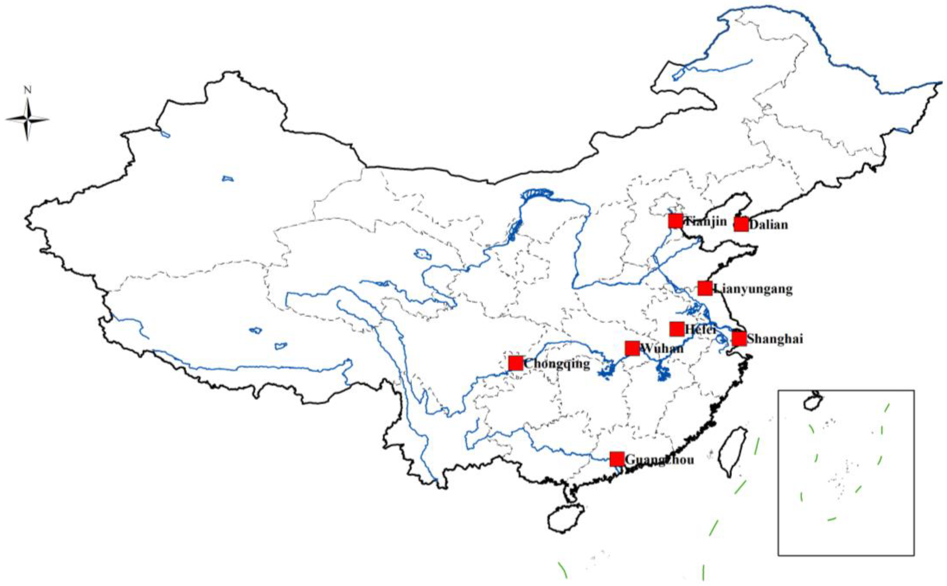
The selection of the consolidation centers in the integrated transportation network under the BRI was evaluated in this paper, with the aim to reduce freight transportation costs and improve the efficiency of logistics operations. First of all, 44 node cities were selected based on the relevant national policies. Then, the transportation networks composed of railway, air, highway, and water routes were constructed. Based on the above work, the corresponding indicators were determined according to complex network theory, and the weights of these indicators were also determined based on the CRITIC approach. Then, the TOPSIS and GRA methods were combined to calculate data on the different transportation modes of each node city. Next, the proportion of the freight volume of the different transportation modes to the total freight volume in 2022 published by the Chinese government was used as the weight of each transportation mode to calculate the comprehensive score of each node city. The results showed that there are the top-ranked node cities in the integrated transportation network are all intersections of the four transportation modes, and most of them are located in inland rivers or coastal areas, indicating that inland river and coastal shipping play an important role in cargo transportation. Additionally, it also indicates that the absence of water transportation weakens the competitiveness of inland cities. Finally, based on the comprehensive consideration, Wuhan, Chongqing, Tianjin, Shanghai, Guangzhou, Lianyungang, Hefei, and Dalian were recommended as the consolidation centers of the integrated transportation network. Moreover, the GRA-TOPSIS method was found to be better than the TOPSIS through Kendall’s tau correlation coefficient and the distinction degree based on the comparison between the GRA-TOPSIS and TOPSIS methods. Additionally, this study can also provide some reference for other countries with transportation networks similar to those of China.
This paper has covered transportation modes such as rail, water, air, and highway when evaluating the consolidation center of the integrated transportation network. However, there are still some limitations that require further study. For example, more factors could be considered when choosing the candidate consolidation centers, such as industrial output value, economic scale, export scale, and the distance between cities. On the other hand, more indicators could be considered for urban population, transportation cost, the impact on urban environments, the carrying capacity of the transportation mode, and the traffic conditions of the node cities in future research. It is hoped that this result can provide some insights for the government to outline and build consolidation centers for an integrated transportation network composed of railway, air, highway, and water routes and for enterprises to choose transportation routes.


