Assessment of Spatial Variability in Ground Models Using Mini-Cone Penetration Testing

Abstract

The assessment of spatial variability in the ground through field experiments has many constraints due to non-homogenous ground conditions and lack of site investigations. For this reason, spatial variability has not been considered in typical analyses. Also, few studies have been conducted on ground spatial variability using models in the laboratory. However, it is necessary to evaluate spatial variability in the ground for more precise analysis and design of construction projects. In this study, in order to evaluate spatial variability in the ground, we performed a number of Mini-Cone Penetration Tests (CPTs) in ground models with one layer of silica sand soil and two layers of silica and weathered soils. Through the Mini-CPTs, cone penetration resistances with depth were measured at many points. Based on the data, the coefficient of variation (CV) and the correlation length (CL) were calculated to quantitatively analyze the vertical and horizontal variability in the ground models. The results showed how the spatial variability in the two ground models varied. This implies that considering spatial variability in the ground can significantly enhance the accuracy of the analysis and design of construction projects.

1. Introduction

The ground on which construction typically occurs encompasses many uncertainties. One factor contributing to these uncertainties is spatial variability [1,2], which implies that drill core samples or the physical and chemical properties of rocks collected from the same location can vary. This difference is one of the primary factors determining the homogeneity or heterogeneity of the ground. Many researchers have elucidated spatial variability in the ground through field tests such as the DHT (Downhole Test), the CPT (Cone Penetration Test), and the SPT (Standard Penetration Test). However, due to practical limitations, construction often proceeds without considering the certainty of these ground properties in most sites [3,4,5,6,7,8,9]).

Additionally, such spatial variability is also used in analyses through numerical modeling. In these numerical analyses, the use of spatial variability is primarily employed when generating random field models. When creating models as random fields for analysis, the spatial variability in the ground cannot be considered by modeling the variables representing ground properties as a single random variable; it is more appropriate to model it as a random field to represent spatial variability [10]. Spatial variability has been studied through numerical analysis for various geotechnical structures. This variability has been theoretically and numerically investigated in relation to strip foundations and pile foundations [11,12,13]. Additionally, various studies have been conducted on slope stability [14,15,16,17], retaining walls [18], and more. Additionally, in evaluating such spatial variability, Zhao et al. [19] proposed a novel method for determining efficient locations for characterizing spatial variability, while Hu and Wang [20] suggested a new non-parametric method using a discrete cosine transform (DCT)-based auto-correlation function (ACF) approach to evaluate the statistical homogeneity of a single CPT data profile, effectively distinguishing heterogeneity without requiring a parametric correlation function.

However, evaluating spatial variability in the ground through field experiments involves many constraints such as uncertain ground conditions. Laboratory tests such as the CPT in a ground model are very useful to better understand spatial variability in the ground. Unlike field experiments, laboratory experiments conducted in a more controlled environment can more precisely determine spatial variability in the ground.

As few studies have been conducted on the evaluation of spatial variability in ground models in the laboratory, in this study, a ground model was constructed in a soil tank, and the cone penetration resistance was measured using the Mini-CPT. In order to investigate the spatial range in which the characteristics of the ground show a strong correlation, the vertical and horizontal spatial variabilities in the ground were assessed through the coefficient of variation (CV) [21] and the correlation length (CL) [22]. The CV is a numerical expression of the uncertainty degree of cone penetration resistance within a soil layer, and the CL is a numerical value that represents the correlation of cone penetration resistance according to the separation distance. In assessing spatial variability, the average values of CV and CL through cone penetration resistance measured in the field could be confirmed through a literature review. The average CV on sand ground was 38% [23], the average vertical CL was 1.6 to 3 m, and the horizontal CL was 14 to 38 m [1,22]. In the case of CL, it is very difficult to compare the CL due to the difference in scale between the field and laboratory. Therefore, it is necessary to compare the results in the field through the CV. As the evaluation of spatial variability through a ground model in the laboratory has rarely been conducted, this study not only provides useful data on spatial variability in ground models but also serves as a measure for determining the appropriateness of evaluating spatial variability through laboratory experiments.

2. Theoretical Background

2.1. Spatial Variability in the Ground

As a natural component, the ground can exhibit variability even in layers that appear homogeneous. This spatial variability arises from various factors such as stress history, characteristics of the samples used, and deposition conditions, serving as a fundamental reason for the uncertainty in ground conditions [1,2]. Variability in the ground does not possess random characteristics, rather it tends to be determined by its spatial location. Expressing spatial variability in the ground with simple statistical figures like mean or variance is insufficient [21]. To understand the correlation of ground properties, two main factors have been primarily used, the CV [21] and CL [22], to delineate the spatial range where the correlation of ground characteristics is expressed. The CV mentioned above is a metric that numerically represents the degree of variation in observed data values within a specific area or space. The CV is used to assess the uniformity or heterogeneity in spatial distribution patterns, measuring how diverse data values are distributed across space. Moreover, the CL in spatial variability can describe the correlation between data points distributed in space. This indicates how data values measured at a specific location are correlated with data values at surrounding locations, revealing how similar or related they are spatially.

2.2. Coefficient of Variation (CV)

The CV is defined as the standard deviation (σ) divided by the mean (μ), representing the numerical uncertainty of an object relatively. It normalizes the variability in data with respect to the mean value, allowing for the comparison of variability among different measurements. The CV for cone penetration resistance within a soil layer can be defined as follows:

$$CV=\left(\frac{\overline{q_c}}{{\mu }_{qc}}\right)$$

(1)

where

• $q_c$ = standard deviation of cone penetration resistance.
• ${\mu }_{qc}$ = mean of cone penetration resistance.

2.3. Correlation Length (CL)

To quantitatively evaluate spatial variability, Padilla and Vanmarcke [24] proposed the concept of CL. CL is a measure that indicates how far the data from a specific point can influence other points. The greater the correlation, the higher the correlation coefficient between adjacent points, and the longer the CL becomes. This implies that certain points can be correlated even if they are far apart from each other. Conversely, if the correlation is low, the CL becomes shorter, indicating that certain points are only correlated when they are in close proximity to each other [25]. The calculation of this CL involves determining the correlation coefficient ($\rho$) of cone penetration resistance between two points separated by a separation distance τ, as shown in the following Equation (2):

$$\rho (\tau )=\frac{{\displaystyle \sum _{h=0}^{{\tau }_{\max -\tau -1}}(q_{c,h}-\overline{q_c})(q_{c,h+\tau }-\overline{q_c})}}{{\displaystyle \sum _{h=0}^{{\tau }_{\max -1}}{(q_{c,h}-\overline{q_c})}^2}}$$

(2)

where

• $q_{c,h}, q_{c,h+\tau }$= a pair of $q_c$ values at two points with a separation distance τ.

CL ($\theta$) is defined as the area under the function based on the relationship between the correlation coefficient $\rho$ and the separation distance τ, and it is calculated according to [21] as follows:

$$\theta ={\int }_{-\infty }^{\infty }\rho \left(\tau \right)d\tau =2{\int }_0^{\infty }\rho \left(\tau \right)d\tau$$

(3)

The correlation coefficient $\rho$ of ground properties converges to 0 as the separation distance increases, and this can be represented through various regression models. The commonly used regression models include the Markovian model (Equation (4)) and the Gaussian model (Equation (5)), where in each model, the CL ($\theta$) is defined by a specific value of the correlation coefficient $\rho$. Although the value of $\rho$ at $\theta$ may differ according to each model, generally, in all models, $\rho$ takes a value less than 0.14. Equations (4) and (5) indicate that the regression coefficient of the regression models is $\theta$, which can be derived through regression analysis such as the least squares method.

$$\rho \left(\tau \right)=\mathrm{e}\mathrm{x}\mathrm{p}\left\{\frac{-2\left|\tau \right|}{\theta }\right\}$$

(4)

$$\rho \left(\tau \right)=\mathrm{e}\mathrm{x}\mathrm{p}\left\{-\pi {\left(\frac{\left|\tau \right|}{\theta }\right)}^2\right\}$$

(5)

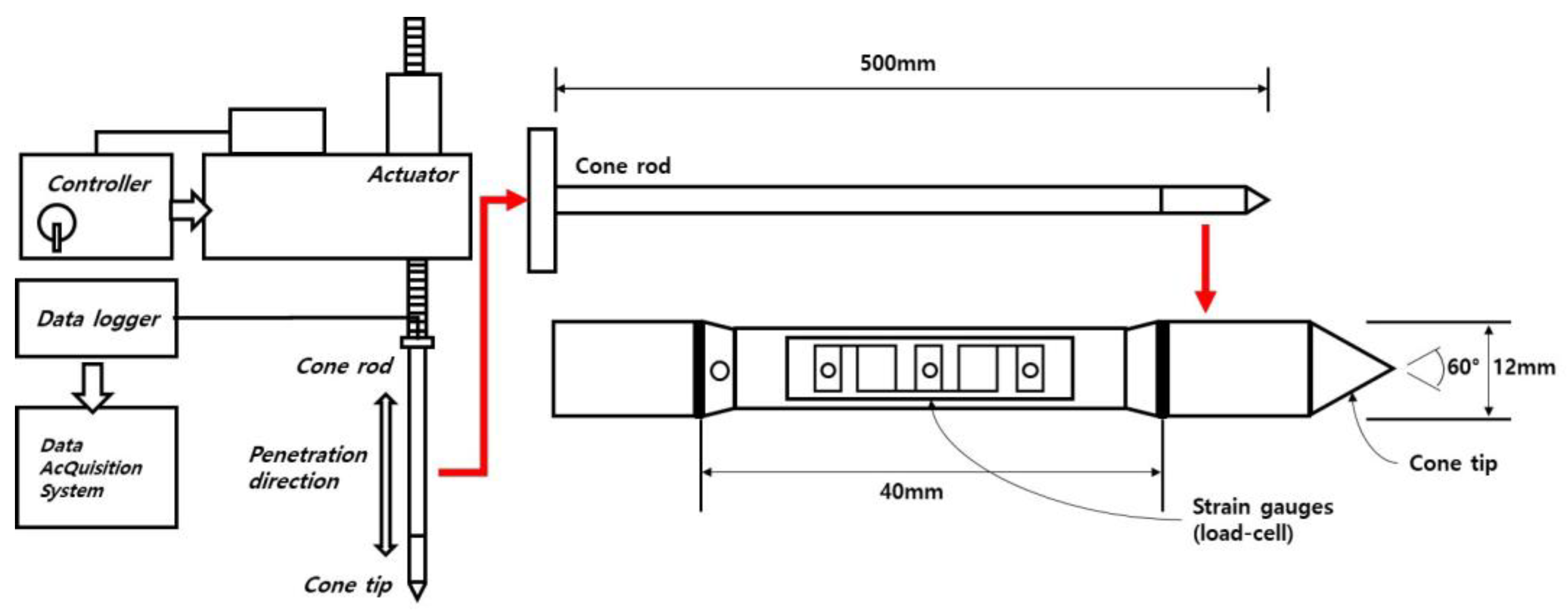
2.4. Mini-Cone Penetration Test (Mini-CPT)

The Cone Penetration Test device was first developed in the Netherlands in the 1930s, and since then, many features have been added with the development of various measurement sensors. Currently, it is used as a representative method for soil investigation alongside the Standard Penetration Test (SPT) [26,27]. The Cone Penetration Test (CPT) is typically conducted in the field and involves inserting a cone with a diameter of 35.7 mm, a penetration area of 100 mm², and a tip angle of 60° into the ground at a constant speed to continuously measure the sleeve friction and cone resistance. The CPT allows for the measurement of cone penetration resistance, sleeve friction, and pore water pressure as the cone is inserted into the ground.

However, the cone penetration equipment used in the field has aspects that make it difficult to use in laboratory experiments due to its size and the complexity of its operation. Due to these difficulties, experiments were conducted using a Mini-CPT developed in the laboratory [28,29,30]. When conducting experiments with this Mini-CPT, four major influencing factors must be considered for cone penetration:

• Cone penetration speed;

The cone penetration speed in sandy ground should be maintained between 2.5 and 20 mm/s [31].

• Distance from the bottom surface of the ground model;

The penetration depth should be far from the distance greater than 10 times the diameter of the cone from the bottom surface [32].

• Distance from the soil tank walls;

The penetration point should be set at a distance greater than 11 times the diameter of the cone from the walls of the soil tank [32].

• Particle size effect ($B/d_{50}$);

A cone with a diameter at least 20 times greater than the average particle size ($d_{50}$) of the ground model should be used [33].

3. Experimental Program

3.1. Soil Index Properties

The soils used for the ground model were silica sand samples and weathered soil samples. To understand the physical properties of the samples, tests such as specific gravity, particle size analysis, compaction, Atterberg limits, and relative density were conducted, and the results are presented in

Table 1. Soil properties.

Sand	Silica Sand	Weathered Soil
$G_s$	2.65	2.69
$e_{max}$	1.06	1.12
$e_{min}$	0.64	0.44
$C_u$	1.03	3.57
$C_g$	1.76	9.28
$\mathrm{U}\mathrm{S}\mathrm{C}\mathrm{S}$	SP	SM

. The soil index properties of the soil samples used in this study are as follows: For the silica sand, the specific gravity ($G_s$) is 2.65, the maximum void ratio ($e_{max}$) is 1.06, the minimum void ratio ($e_{min}$) is 0.64, the uniformity coefficient ($C_u$) is 1.03, and the coefficient of curvature ($C_g$) is 1.76; the sand is classified as SP (poorly graded sand) according to the unified soil classification system (USCS). The weathered soil has a $G_s$ of 2.67, $e_{max}$ of 1.12, $e_{min}$ of 0.44, $C_u$ of 3.57, and $C_g$ of 9.28; the soil is classified as SM (silty sand) according to the USCS.

3.2. Technical Specifications

Figure 1 shows the CPT used in the experiment. The CPT used is a Mini CPT, which is a smaller version of the CPT typically used in the field, and its structure is shown in Figure 1. The cone has a diameter of 12 mm, a tip angle of 60°, and a rod length of 500 mm. It was constructed using four strain gauges attached in a 4-bridge manner on the load cell part and is connected to a data logger for measurements. Furthermore, penetration is conducted through an actuator, allowing for a maximum penetration speed of up to 20 mm/s.

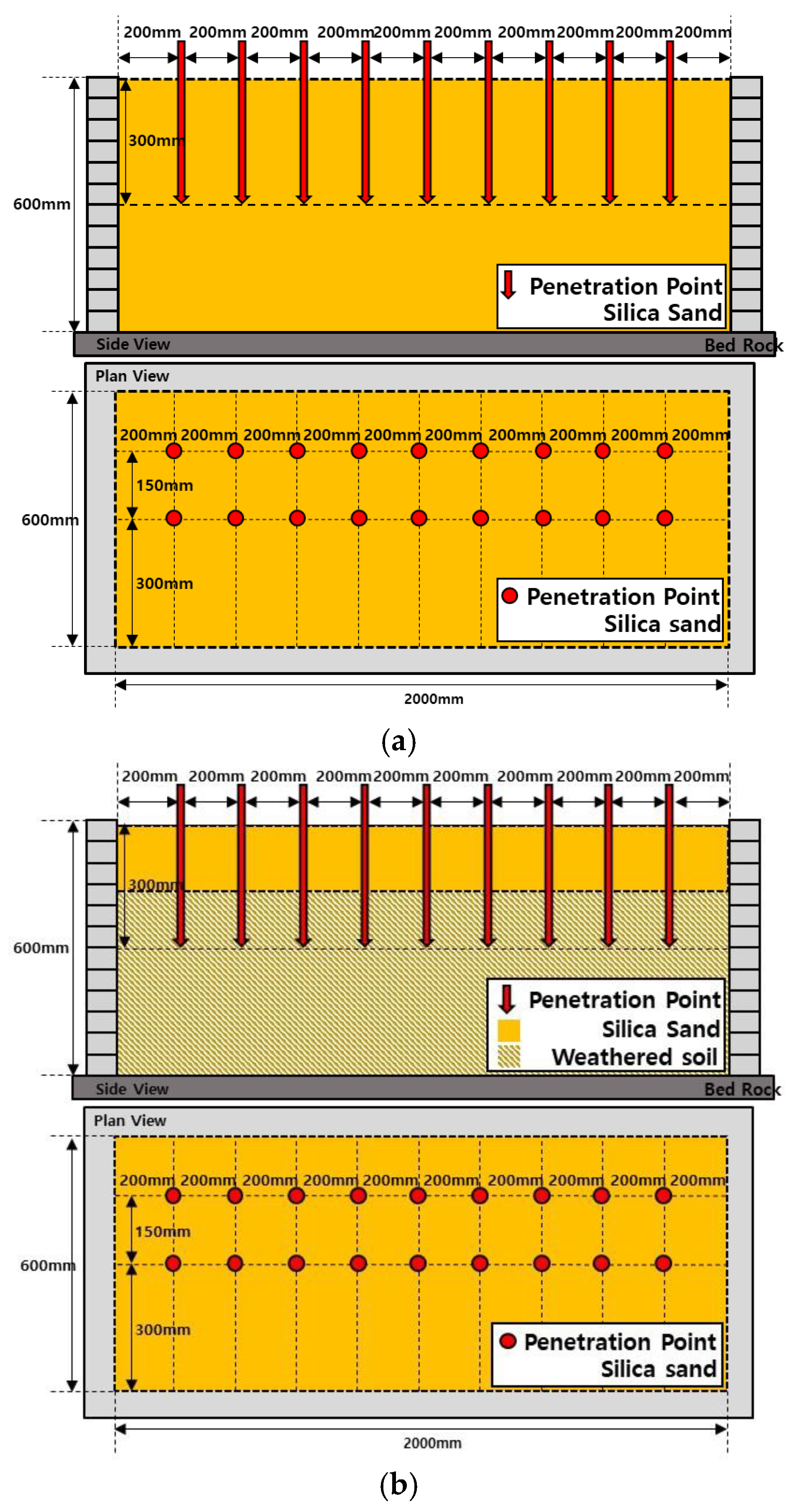
3.3. Ground Models

A soil tank with dimensions of 2000 × 600 × 600 mm was used to construct the ground model, as shown in Figure 2. The experiment was conducted using silica sand and weathered soil samples, as mentioned in Section 3.1. Each soil sample had a water content of 0%. The ground model was designed considering the penetration depth of the cone. Penetration was conducted at a total of 18 locations, with the 30 cm point designated as A and the 45 cm point as B. The spatial variability in the ground model was evaluated using the cone penetration resistance data from all 18 locations through calculations of CV and CL.

Figure 2a consists of a single ground layer of silica sand with a relative density of 75%, and the composition was made homogeneously to validate the results of spatial variability in the ground model through the coefficient of variance and vertical CL. Figure 2b shows a two-layer ground composed of silica sand and weathered soil. For the weathered soil layer, the composition was conducted with a relative density of 95%, and for the silica sand layer, with a relative density of 75%. The depth of the silica sand layer was set to 15 cm considering the cone penetration depth.

The construction of the sandy grounds for Case 1 and Case 2 was carried out as uniformly as possible by dropping the sand through the pluviation system.

Accounting for the considerations for the Cone Penetration Tests mentioned in Section 2.4, the penetration points were determined. The Cone Penetration Tests were conducted outside the influence range of the walls and bottom surface, with a penetration speed of 20 mm/s. The cone penetration points were designated as point A at the 30 cm location and point B at the 45 cm location.

4. Discussion of the Results

4.1. CPT Test Results

Figure 3a shows the results of cone penetration resistance for Case 1′s single silica sand ground, and Figure 3b presents the results for Case 2′s multi-layered ground of silica sand and weathered soil. As shown in Figure 3a,b, the cone resistance for a single soil layer has less variation in $q_c$ values than that for the two soil layers. This appears to be due to the fact that the silica sand has a more uniform particle size distribution than the weathered soil. Additionally, the variability between the two ground models might have been due to the pluviation system that was used to homogeneously compose the silica sand ground, while compaction was carried out to compose the weathered soil ground.

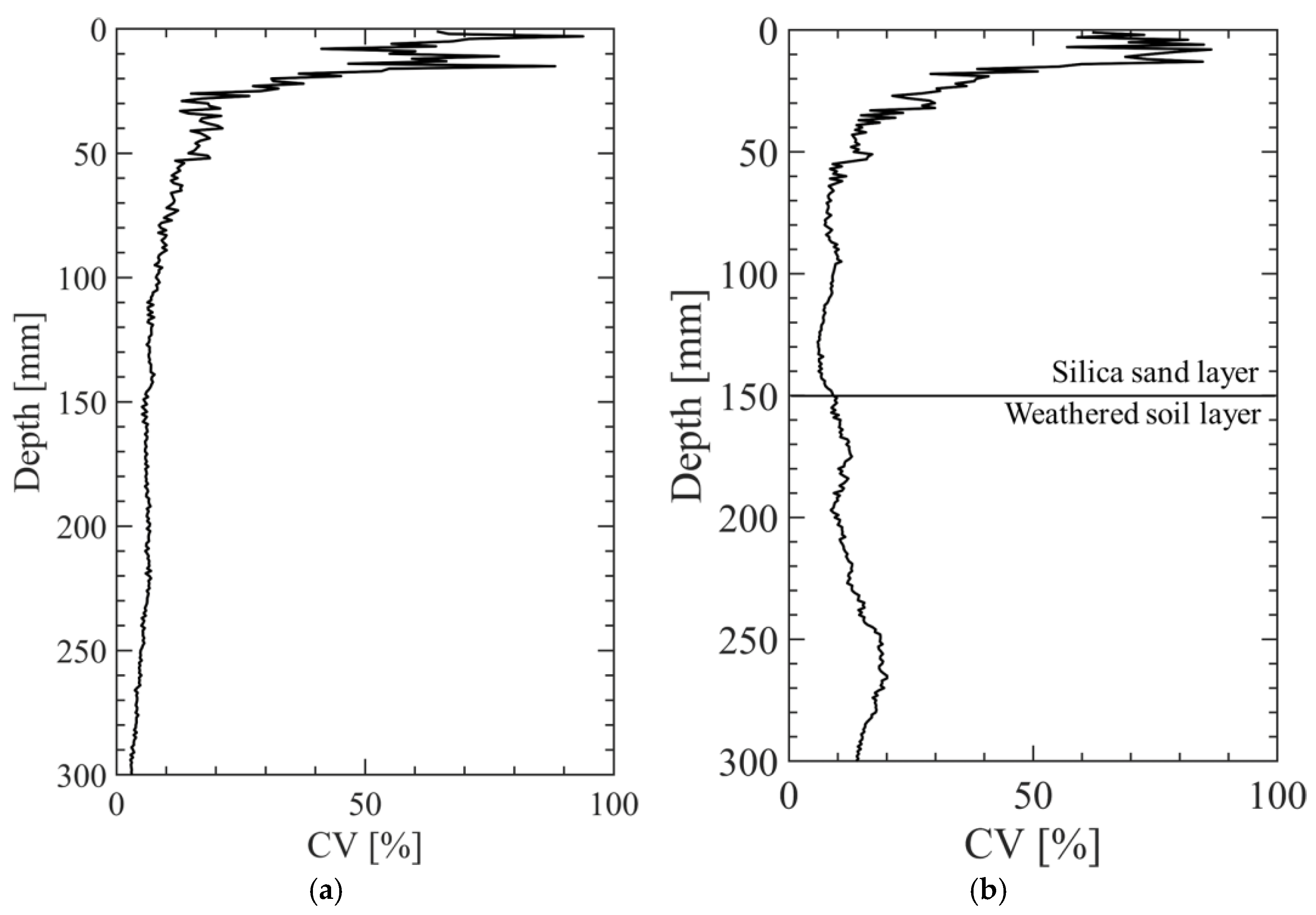
4.2. CV Analysis

Figure 4 presents the horizontal CV results for the Cone Penetration Test, calculated using Equation (1). The calculation of the horizontal CV was conducted by dividing the cone penetration resistance measurement results into 1 mm intervals. Note that, although the ground models in the laboratory were prepared as uniformly as possible, the qc values are quite varied for the different points at the same depths. This implies that there may be a lot more considerable spatial variability in the field than in the lab.

Figure 4a shows the horizontal CV results for Case 1. A relatively high CV was observed up to a depth of 50 mm due to the influence of low confining pressure. The high CV in this initial section was deemed unreliable due to the low confining pressure, so the analysis was conducted using data below 50 mm. For this depth, the CV ranged from 2.21 to 18.78% with an average CV of 6.76%, indicating significantly smaller variability with increasing depth.

Figure 4b presents the horizontal CV results for Case 2. The CV in the silica sand layer ranged from 5.87 to 17.02%, with an average variability of 8.38%, while in the weathered soil layer, it ranged from 8.58 to 20.08%, with an average CV of 13.70%. The higher CV in the weathered soil layer below 150 mm is attributed to the varied particle sizes and void ratio in the weathered soil collected from the field, unlike the silica sand ground. This is considered to reflect the differences that occurred during the construction of the ground models.

The coefficient of variation (CV) in field ground is known to exhibit an average variation of 38%. However, in this study, the homogeneously created silica sand ground model showed CV values of approximately 6.76% and 8.38%, while the weathered soil ground model showed CV values of approximately 13.70%. This resulted in a difference in variability of 31.24%, 29.62%, and 24.3%, respectively, compared to the average CV in the field. The reason for this is believed to be the characteristics of the ground at the site, such as layered structures and particle distribution, which differ from artificially created ground models in laboratories, leading to somewhat different CV values at the site.

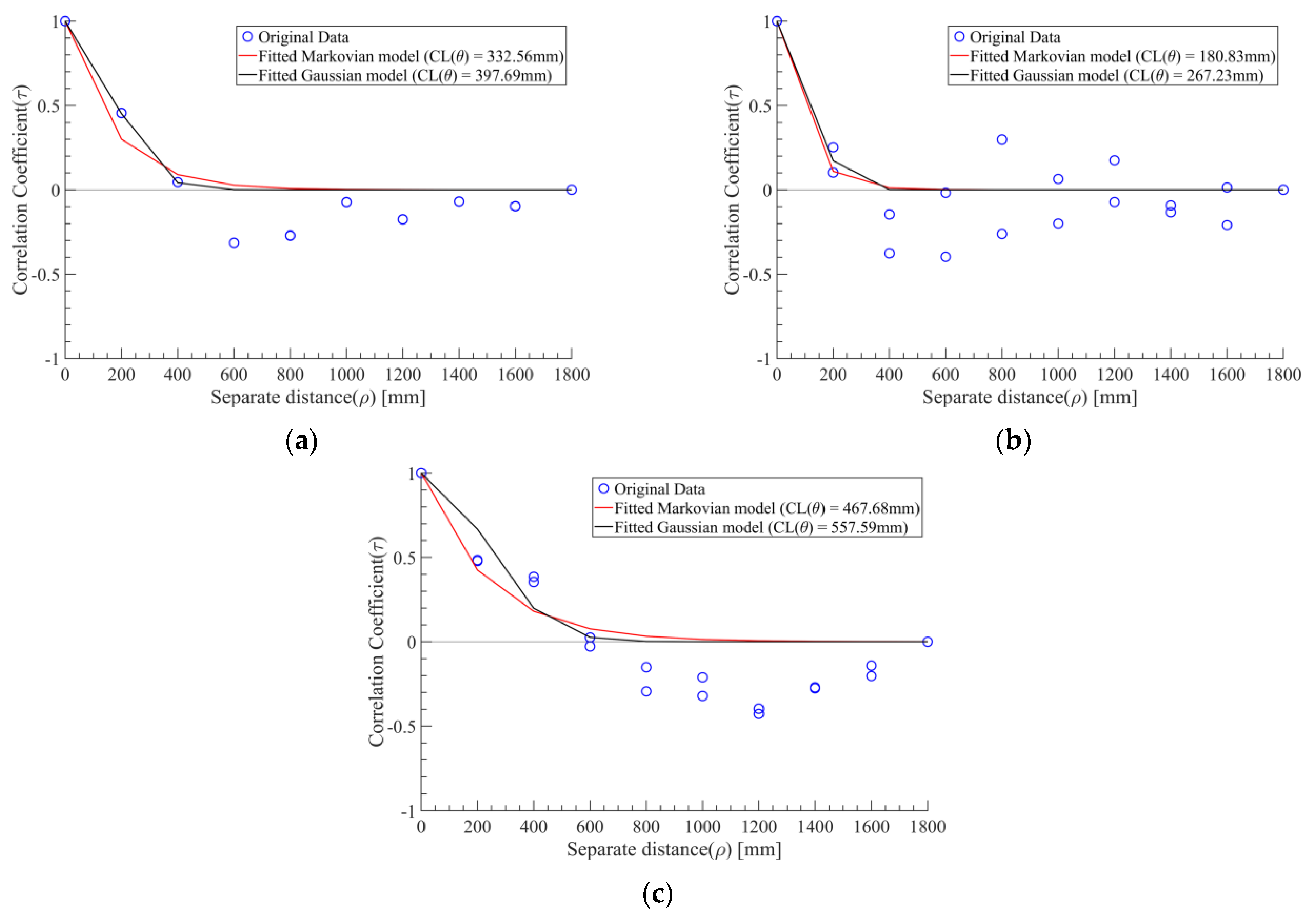
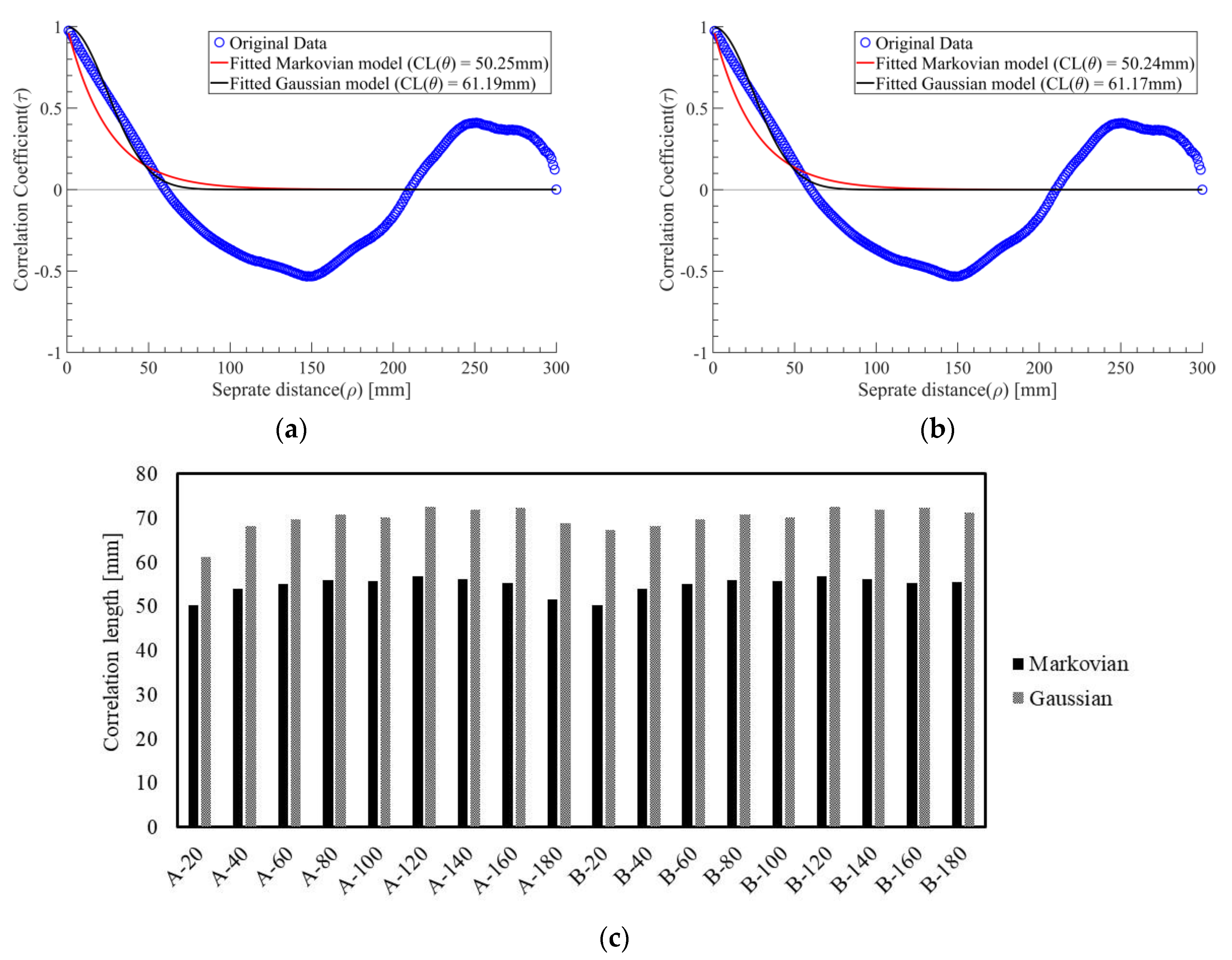
4.3. CL Analysis

4.3.1. Horizontal CL

Figure 5 presents the horizontal CLs for Case 1 and Case 2. The horizontal CL was calculated by taking the average of the measured cone penetration resistances at each of the 18 locations. Figure 5a presents the CL for the silica sand layer, and Figure 5b,c separate the calculations of CLs for silica sand and weathered soil grounds, respectively. For the application of the CL model, Markovian and Gaussian models were utilized in the calculations.

As can be seen from Figure 5a, the horizontal CLs using the Markovian model and the Gaussian model were found to be 332.56 mm and 397.69 mm, respectively. Figure 5b shows the calculation results for the horizontal CLs in the silica sand layer, with the Markovian model and the Gaussian model yielding 180.83 mm and 267.23 mm, respectively. Figure 5c displays the calculation results for the horizontal CLs in the weathered soil layer, with the Markovian model and the Gaussian model resulting in 467.68 mm and 557.59 mm, respectively.

The comparative analysis of the horizontal CLs for Case 1 and Case 2 revealed that the silica sand ground exhibited smaller CLs in Case 2 than those in Case 1, despite the CV. Moreover, although larger CLs were expected in the silica sand ground due to greater variability in the weathered soil ground, smaller CLs were calculated for the silica sand ground compared to the weathered soil ground. As shown in Figure 5a,b, this smaller CL observed in the silica sand ground for Case 2 is considered to be influenced by the penetration depth. Additionally, the impact of having fewer data points, as opposed to calculating vertical CLs, is also thought to be a factor.

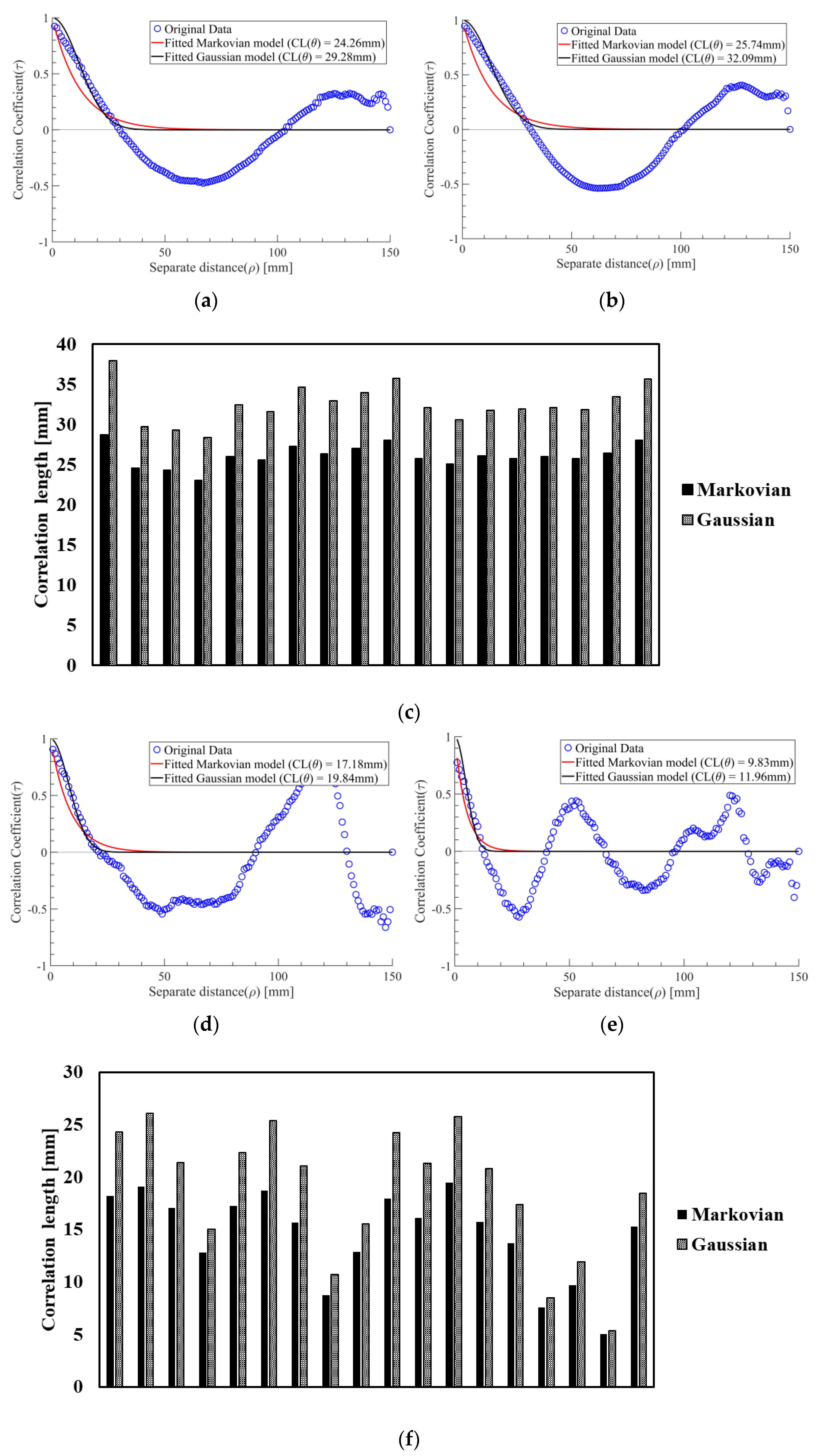
4.3.2. Vertical CL

Figure 6 shows the vertical correlation lengths of two points as a representative example for Case 1 silica sand ground and Figure 6c shows the CLs for all measured points. The vertical CLs for each point were calculated with a spacing of 1 mm, and the results for each location are presented in Figure 6c.

Each fitted vertical CL was found to be 97.76 mm on average for the Markovian model and 134.60 mm for the Gaussian model. Furthermore, the vertical CLs were calculated within a range of 96.61 to 98.74 mm for the Markovian model and 133.24 to 135.62 mm for the Gaussian model. The CV for each model was 0.68% and 0.59%, respectively, indicating that the CLs at each point were very consistent.

These minor differences can be attributed to the homogeneity of the ground models, as mentioned in Section 3.3. Therefore, it is considered that these vertical CL results enhance the reliability of the CL calculations performed on the ground models in this study.

Figure 7 shows the vertical CLs for Case 2. Similar to the calculation of horizontal CLs, calculations were conducted separately for the silica sand layer and the weathered soil layer. Figure 7c,f display the vertical CLs for each location.

Figure 7a,b represent the vertical CLs for representative points in the silica sand layer, and Figure 7c shows the CLs for all measured points. Based on the results from 18 penetration points, the vertical CLs in the sand layer were calculated to be an average of 26.09 mm for the Markovian model and an average of 35.55 mm for the Gaussian model. They varied within the ranges of 23.01 to 28.72 cm and 28.36 to 37.93 cm, respectively, with coefficients of variation measuring 1.18% and 1.14%. It was observed that the variability was very low.

Figure 7c,d represent the vertical CLs for representative points in the weathered soil layer, and Figure 7f shows the CLs for all measured points. The vertical CLs in the weathered soil layer were calculated to be an average of 14.49 cm for the Markovian model and an average of 18.64 cm for the Gaussian model based on natural conditions. They varied within the ranges of 5.05 to 19.5 cm and 5.33 to 26.11 cm, respectively, with CV measuring 29.46% and 33.63%. This higher variability is attributed to the natural state of the weathered soil layer, which exhibits variations in particle sizes and pore structure compared to the artificially homogenized structure of the silica sand layer.

5. Conclusions

To evaluate spatial variability in uncertain ground conditions, it is challenging to conduct field experiments. Therefore, we investigated the spatial variability in two types of ground models. Using a Mini-Cone Penetration Test apparatus, cone penetration resistances were measured at each location. Based on the measured cone penetration resistances, coefficients of variation, and vertical and horizontal CLs were calculated. The conclusions of this study are as follows:

• Below the 50 mm threshold, the coefficient of variation (CV) was found to be relatively stable. Especially, in the silica sand ground model, the average CV was measured at 6.76%, indicating minimal variability and suggesting a well-composed homogeneous ground model. In contrast, the weathered soil ground model exhibited a CV of 13.70%, showing a comparatively higher level of variability than that of the silica sand ground model.
• The horizontal CL was calculated using the average cone penetration resistance measured at each point. The CL for the silica sand ground in the two-soil layer was calculated to be smaller than that for the silica sand ground in the single soil layer and the weathered soil ground in the two-soil layer. This is believed to be due to the lower penetration depth in the silica sand ground of the two-soil layer, and the impact of having fewer data points (smaller separation distances). This suggests that further research may be needed, such as conducting experiments with more data points or deeper penetration.
• In the calculation of vertical CLs, the CV for the silica sand layer was observed to be very low, confirming the validity of the CL calculations. In contrast, the CV for the weathered soil layer was relatively high. This is believed to be a result of the homogeneous particles of the silica sand layer and the various particles of the weathered soil layer, which are considered to be the primary influencing factors on vertical CLs.
• The results of this experiment, conducted under the assumption of a homogeneously built ground model, revealed that the ground model exhibits less variability compared to the average variability observed in the field. The observed variability suggests that evaluating spatial variability through field and laboratory tests requires careful consideration of the non-homogeneity present in field conditions.

Although it is very important to consider spatial variability for the accurate evaluation of soil behavior, spatial variability in soils in the reduced scaled tests such as the 1 g shaking table test has rarely been considered. The results obtained from this study such as the CV and CL values can be used for further numerical study considering spatial variability. Obtaining the CV and CL values for various ground models in the laboratory can enhance the accuracy of the numerical study of spatial variability in soils.

References

- Lacasse, S.; Nadim, F. Uncertainties in Characterizing Soil Properties. In Uncertainty in the Geologic Environment: From Theory to Practice; Shackleford, C.D., Nelson, P.P., Roth, M.J.S., Eds.; ASCE Geotechnical Special Publication: Reston, VA, USA, 1996; pp. 49–75. [Google Scholar]
- Elkateb, T.; Chalaturnyk, R.; Robertson, P.K. An Overview of Soil Heterogeneity: Quantification and Implications on Geotechnical Field Problems. Can. Geotech. J. 2002, 40, 1–15. [Google Scholar] [CrossRef]
- Griffiths, D.V.; Fenton, G.A. Bearing Capacity of Spatially Random Soil: The undrained Clay Prandtl Problem Revisited. Geotechnique 2001, 51, 351–359. [Google Scholar] [CrossRef]
- Koutsourelakis, S.; Prevost, J.H.; Deodatis, G. Risk Assessment of an Interacting Structure-soil System due to Liquefaction. Earthq. Eng. Struct. Dyn. 2002, 31, 851–877. [Google Scholar] [CrossRef]
- Haldar, S.; Babu, G.L.S. Effect of Soil Variability on the Response of Laterally Loaded Pile in Undrained Clay. Comput. Geotech. 2007, 35, 537–547. [Google Scholar] [CrossRef]
- Lenz, J.A.; Baise, L.G. Spatial variability of liquefaction potential in regional mapping using CPT and SPT data. Soil Dyn. Earthq. Eng. 2007, 27, 690–702. [Google Scholar] [CrossRef]
- Vivek, B.; Raychowdhury, P. Probabilistic Approach for Evaluation of Soil Liquefaction Considering Spatial Variability of Soil. In Proceedings of the Indian Geotechnical Conference, Kochi, India, 15–17 December 2011. [Google Scholar]
- Cho, S.E. Probabilistic analysis of seepage that considers the spatial variability of permeability for an embankment on soil foundation. Eng. Geol. 2012, 133–134, 30–39. [Google Scholar] [CrossRef]
- Saygili, G. Probabilistic Assessment of Soil Liquefaction Considering Spatial Variability of CPT Measurements. Georisk 2016, 11, 197–207. [Google Scholar] [CrossRef]
- Cho, S.E.; Park, H.C. Probabilistic Stability Analysis of Slopes by the Limit Equilibrium Method Considering Spatial Variability of Soil Property. J. Korean Soc. Geotech. Eng. 2009, 25, 13–25. [Google Scholar]
- Jaksa, M.B.; Goldsworthy, J.S.; Fenton, G.A.; Kaggwa, W.S.; Griffiths, D.V.; Kuo, Y.L.; Poulos, H.G. Towards reliable and effective site investigations. Géotechnique 2005, 55, 109–121. [Google Scholar] [CrossRef]
- Suchomel, R.; Masín, D. Comparison of different probabilistic methods for predicting stability of a slope in spatially variable c–φ soil. Comput. Geotech. 2015, 37, 132–140. [Google Scholar] [CrossRef]
- Naghibi, F.; Fenton, G.A.; Griffiths, D.V. Probabilistic considerations for the design of deep foundations against excessive differential settlement. Can. Geotech. J. 2016, 53, 1167–1175. [Google Scholar] [CrossRef]
- Griffiths, D.V.; Fenton, G.A. Three-dimensional seepage through spatially random soil. J. Geotech. Geoenviron. Eng. 1997, 123, 153–160. [Google Scholar] [CrossRef]
- Hicks, M.A.; Spencer, W.A. Influence of heterogeneity on the reliability and failure of a long 3D slope. Comput. Geotech. 2016, 37, 948–955. [Google Scholar] [CrossRef]
- Li, Y.J.; Hicks, M.A.; Vardon, P.J. Uncertainty reduction and sampling efficiency in slope designs using 3D conditional random fields. Comput. Geotech. 2016, 79, 159–172. [Google Scholar] [CrossRef]
- Tom, D.G.; Philip, J.V.; Michael, A.H. Assessment of soil spatial variability for linear infrastructure using cone penetration test. Géotechnique 2021, 71, 999–1013. [Google Scholar]
- Sert, S.; Luo, Z.; Xiao, J.H.; Gong, W.P.; Juang, C.H. Probabilistic analysis of responses of cantilever wall-supported excavations in sands considering vertical spatial variability. Comput. Geotech. 2016, 75, 182–191. [Google Scholar] [CrossRef]
- Zhao, T.; Wang, Y.; Xu, L. Efficient CPT locations for characterizing spatial variability of soil properties within a multilayer vertical cross-section using information entropy and Bayesian compressive sensing. Comput. Geotech. 2021, 137, 104260. [Google Scholar] [CrossRef]
- Hu, Y.; Wang, Y. Evaluating statistical homogeneity of cone penetration test (CPT) data profile using auto-correlation function. Comput. Geotech. 2024, 165, 105852. [Google Scholar] [CrossRef]
- Vanmarcke, E.H. Random Fields: Analysis and Synthesis; The MIT Press: Cambridge, MA, USA, 1983. [Google Scholar]
- DeGroot, D.J.; Baecher, G.B. Estimating Autocovariance of In-situ Soil Properties. J. Geotech. Eng. 1993, 119, 147–166. [Google Scholar] [CrossRef]
- Jones, A.L.; Steven, L.K.; Perdo, A. Estimation of Uncertainty in Geotechnical Properties for Performance-Based Earthquake Engineering; Pacific Earthquake Engineering Reserch Center, College of Engineering, University of California: Los Angeles, CA, USA, 2002. [Google Scholar]
- Padilla, J.D.; Vanmarcke, E.H. Settlement of Structures on Shallow Foundations; Research Report R74-9; Department of Civil Engineering, MIT: Cambridge, UK, 1974. [Google Scholar]
- Onyejekwe, S.; Kang, X.; Ge, L. Evaluation of the scale of fluctuation of geotechnical parameters by autocorrelation function and semivariogram function. Eng. Geol. 2016, 214, 43–49. [Google Scholar] [CrossRef]
- Robertson, P.K.; Campanella, R.G. Guidelines for Geotechnical Design Using CPT and CPTU; University of British Columbia, Vancouver, Department of Civil Engineering, Soil Mechanics Series: Vancouver, BC, Canada, 1988. [Google Scholar]
- Lunne, T.; Robertson, P.K.; Powell, J.J.M. Cone Penetration Testing in Geotechnical Practice; Chapman & Hall: London, UK, 1997. [Google Scholar]
- Kim, H.J.; Kim, D.J.; Kim, D.S.; Choo, Y.W. Development of Miniature Cone and Characteristics of Cone Tip Resistance in Centrifuge Model Tests. J. Korean Soc. Civ. Eng. 2013, 33, 631–642. [Google Scholar]
- Kim, J.H.; Choo, Y.W.; Kim, D.J.; Kim, D.S. Miniature Cone Tip Resistance on Sand in a Centrifuge. J. Geotech. Geoenvironmental. Eng. 2016, 142, 04015090. [Google Scholar] [CrossRef]
- Jeong, S.G.; Moon, M.S.; Kim, D.H. Applicability of Mini-Cone Penetration Test Used in a Soil Box. J. Korean Geosynth. Soc. 2023, 22, 83–92. [Google Scholar]
- Bolton, M.D.; Gui, M.W.; Garnier, J.; Corte, J.F.; Bagge, G.; Laue, J.; Renzi, R. Centrifuge cone penetration tests in sand. Géotechnique 1999, 49, 543–552. [Google Scholar] [CrossRef]
- Been, K.; Crooks, J.H.A.; Becker, D.E.; Jefferies, M.G. The cone penetration test in sands: Part I, state parameter interpretation. Geotechnique 1986, 36, 239–249. [Google Scholar] [CrossRef]
- Gui, M.W.; Bolton, M.D.; Garnier, J.; Corte, J.F.; Bagge, G.; Laue, J.; Renzi, R. Guidelines for cone penetration tests in sand. Centrifuge 1998, 98, 1998. [Google Scholar]