Abstract
Miniature loudspeakers exhibit pronounced nonlinear characteristics due to physical size limitations and the demand for sufficient sound pressure. The primary nonlinear properties, including the force factor, mechanical stiffness, and mechanical resistance, depend on the displacement or velocity of the voice coil. The creep effect in the loudspeaker’s suspension system, which significantly affects low-frequency displacement, is often neglected in existing studies on nonlinear dynamics. This study enhances the modeling of miniature loudspeakers by incorporating the creep effect into an extended nonlinear model. The voice coil displacement and total harmonic distortion (THD) predicted by the extended model were validated against experimental data. The displacement and THD values predicted by the nonlinear model in consideration of the creep effect corresponded closely to the actual measurement values, substantiating the effectiveness and precision of the model.
1. Introduction
Miniature loudspeakers are crucial sound-emitting components in mobile phones, headphones, and other portable audio devices. As the demand for compact portable audio devices with high sound output continues to grow, miniature loudspeakers increasingly operate under large signal conditions, leading to nonlinearities and consequent harmonic distortions. Additionally, with the requirements for good sound quality and the emergence of new near-ear open devices like AR/VR headsets, the nonlinear performance at low frequencies has also gained attention. Thus, investigating the nonlinear performance of miniature loudspeakers, including the low frequency range, is particularly significant. Theoretical models capable of accurately predicting nonlinear performance are needed to provide a foundation for displacement prediction, distortion compensation, and other performance enhancements.
Previous studies have modeled and analyzed the nonlinear behavior of loudspeaker systems [1,2,3,4]. Klippel expanded the widely employed lumped-parameter linear model into a nonlinear form [5,6], delineated the principal nonlinear parameters of the loudspeaker system, and proposed methods for measuring these nonlinear parameters. Klippel also analyzed the harmonic distortion and other effects induced by nonlinearities. Subsequently, Dobruchi et al. numerically analyzed the nonlinear distortion in loudspeakers [7]. Bai proposed a method for diagnosing speaker unit faults based on the measurement of nonlinear distortions [8]. However, these nonlinear models do not consider the creep effect, which is a typical viscoelastic property in the suspension systems of miniature loudspeakers.
The creep effect refers to the gradual increase in deformation over time in the suspension system of a loudspeaker subjected to external forces [9]. As a result, displacement increases at low frequencies, which is an effect that is particularly evident in miniature loudspeakers with composite membranes. The models developed to evaluate the creep effect can mainly be classified into three types. The first type is the logarithmic empirical model proposed by Knudsen based on measurements and mathematical analysis [10,11]. Klippel subsequently improved the empirical model [12] and integrated it into the testing of small-signal linear parameters. However, this type of model is only applicable to frequency domain analysis [13,14], and it cannot be extended to time domain calculations. The second type of model involves the incorporation of the standard linear solid (SLS) model from linear viscoelastic mechanics into the small-signal analysis of loudspeakers while using Newtonian dashpots and Hookean springs to describe creep [15]. This model is applicable to both frequency and time domain analyses. However, most applications of this model are transfer-function-based frequency domain analysis [16,17,18,19,20], which is limited to the linear characteristics of the loudspeaker [16] and cannot be used for nonlinear calculations. The third type of model is the fractional derivative model, and existing research has demonstrated its applicability in describing the creep effect in loudspeaker systems [21]. Subsequent studies have also developed corresponding identification algorithms, providing methods for analyzing the nonlinear performance of loudspeaker systems based on this model [22]. Although this model allows for nonlinear analysis, it exhibits memory characteristics, is unable to run in real time, and demands high computational resources, thereby limiting its practical application for active control.
To enable computationally efficient, real-time evaluations of the nonlinear performance of miniature loudspeakers in consideration of the creep effect, we extended the nonlinear model of miniature loudspeakers by incorporating the SLS model. The accuracy of the new nonlinear model incorporating creep was then assessed through comparison with experimental results.
2. Nonlinear Model with Creep
2.1. Equivalent Circuit Model
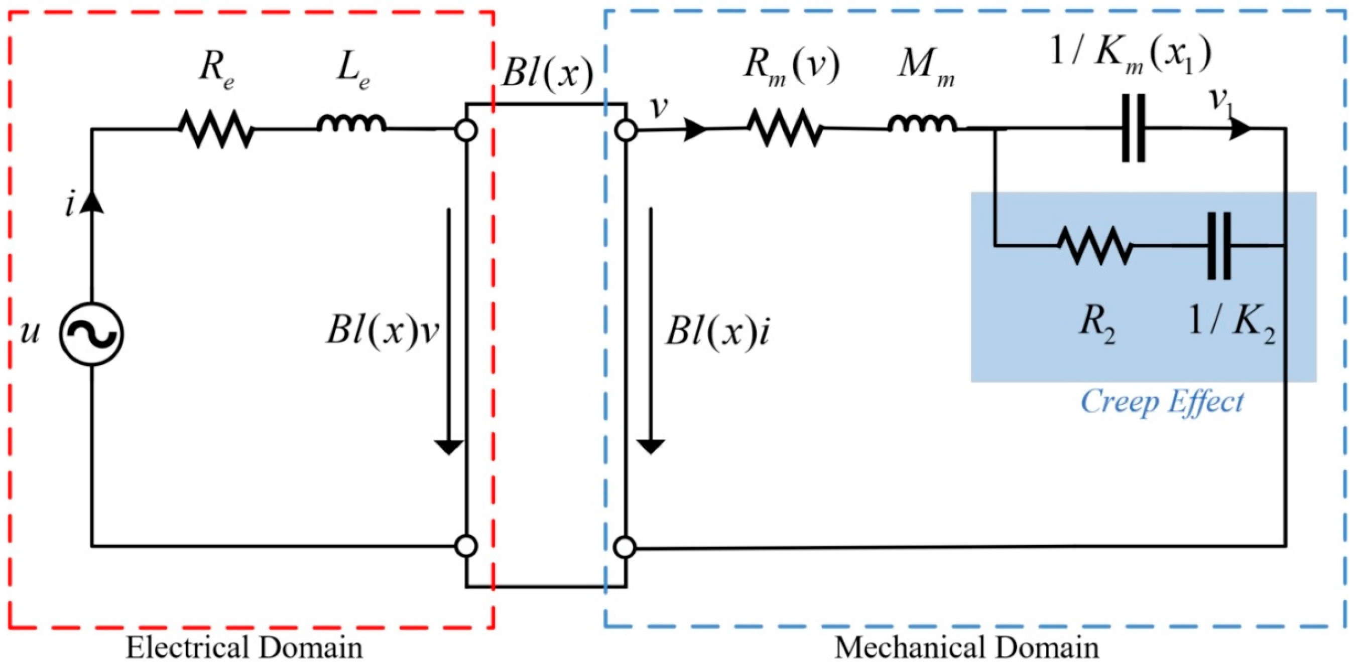
We focused on moving-coil miniature loudspeakers because these are the most common type of miniature loudspeakers. These miniature loudspeakers can be modeled by an equivalent circuit when the wavelength is large compared to the geometric dimensions [8]. The electrical equivalent circuit diagram of the nonlinear model with creep (referred to as the NL-C model) is depicted in Figure 1. In addition to the commonly included electrical and mechanical components, the NL-C model also incorporates the SLS model from viscoelastic mechanics to characterize the creep effect [16]. In the NL-C model, the loudspeaker suspension is considered as a combination of elastic and viscous properties. Therefore, a secondary stiffness and a secondary damper were introduced and could be adjusted to increase the displacement at low frequencies, thereby simulating the creep effect.

Figure 1.
Equivalent circuit of the NL-C model.
As shown in Figure 1, the electrical part of the system (enclosed within the red dashed line) is modeled by the voice coil inductance Le and electrical voice coil resistance at direct current (DC) Re. The mechanical part (enclosed within the blue dashed line) is modeled by the mechanical resistance Rm, moving mass Mm, and mechanical stiffness Km. The electrical and mechanical parts are coupled by the magnetic force factor Bl. In this model, the acoustic part is neglected because it is negligibly small when compared with the other two parts. The secondary damper R2 and the secondary stiffness K2 in the blue shaded area are connected in parallel with mechanical stiffness Km, representing the suspension creep of the miniature loudspeaker. It should be noted that if R2 and K2 are disregarded (i.e., considered to be infinitely large), the NL-C model degenerates into the nonlinear model without creep (referred to as the NL-NC model) that has been used for nonlinear analysis in the previous study [6].
2.2. State–Space Method
Based on the equivalent circuit in Figure 1, the NL-C model is represented by the following three loop equations:
where u denotes the voltage applied across the system, i represents the current flowing through the voice coil, v is the velocity of the voice coil, x is the displacement of the diaphragm, v1 corresponds to the equivalent velocity through the mechanical stiffness Km (as seen in Figure 1), and x1 is the equivalent displacement associated with v1. The parameters Bl, Km, and Rm are commonly considered as nonlinear parameters that depend on the displacement and velocity and are expressed by the following polynomials [6]:
where and are modeled as a fourth-order approximation, while is modeled using a second-order approximation, consistent with the Klippel LSI (Large Signal Identification) module.
Let , , then Equations (2) and (3) can be rewritten as follows:
Choosing as the state vector allows for the reformulation of Equation (1), along with Equations (7) and (8), into the following state–space representation:
where represents the derivative of the state vector , , as well as the following:
With the sampling period denoted as Ts, discretization is conducted using the backward difference method according to Equation (9). Consequently, the state parameters at time instance n + 1 can be computed based on those at time instance n as follows:
where:
2.3. Performance Prediction
In practice, the parameters of a known speaker (e.g., Re, Le, Mm, Km, Bl, and Rm) can be easily obtained through measurement, while K2 and R2 can be derived by fitting the measurement data [16]. In this case, the state variables of the NL-C model can be obtained by Equation (11).
Subsequently, the sound pressure response of the miniature loudspeaker can be calculated using the following formula:
where r denotes the distance between the sound emission point of the miniature loudspeaker and the test point, A is the effective radiating area, is the air density, is the sound velocity in air, j is the imaginary unit, and f is the frequency of the excitation signal. Due to the nonlinear factors within the loudspeakers, nonlinear distortions will be generated in the sound pressure output response. Total harmonic distortion (THD) is commonly used to quantify the amount of harmonic distortion present in the output signal when a pure input signal is applied. It can then be calculated as follows:
where Pt(f) and P(nf) represent the total sound pressure and the nth harmonic component in the complex sound pressure signal, respectively. Generally, a lower THD indicates that the loudspeaker more accurately reproduces the original signal, resulting in clearer and more precise sound.
It is worth noting that the NL-C model degrades to the NL-NC model when K2 and R2 tend toward infinity and the secondary branch describing creep becomes open-circuited. Accordingly, the nonlinear performance of the NL-NC model can also be evaluated.
3. Experimental Validation
3.1. Experimental Setup
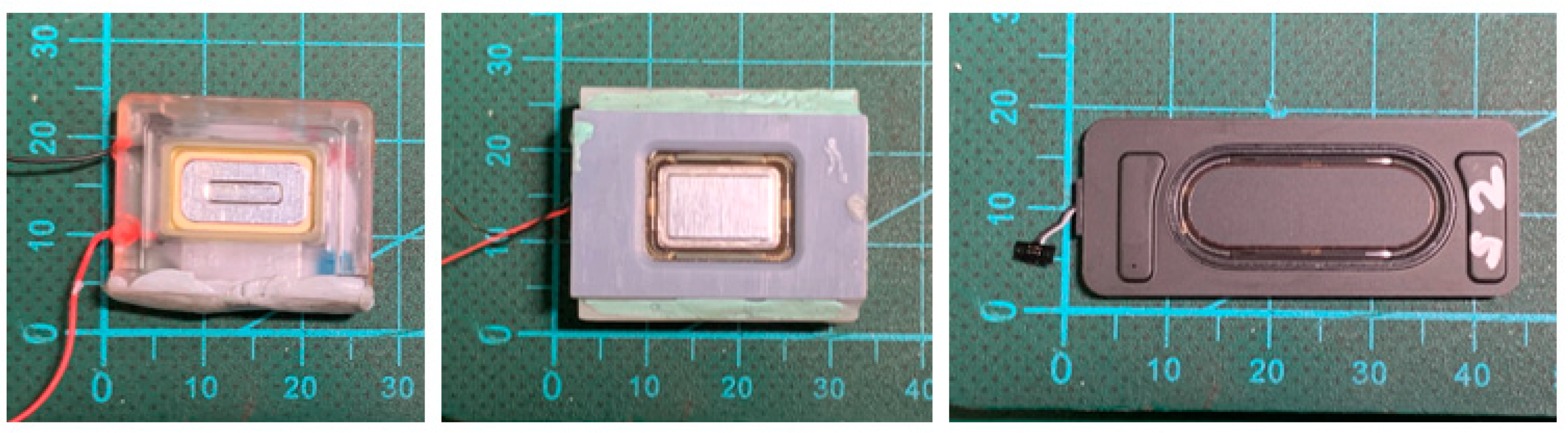
Experiments were conducted on three miniature loudspeaker samples to assess the effectiveness of the NL-C model. Figure 2 depicts the front views of the three samples. Based on the parameters of the loudspeaker samples measured using a Klippel R&D system (Klippel GmbH, Dresden, Germany), the nonlinear displacement waveforms and THD were predicted using the NL-C model and degraded NL-NC model and measured experimentally under the same nonlinear conditions after all the samples achieved a stable operating state. The predictions were then compared with the measurement values.

Figure 2.
Front views of the three miniature loudspeaker samples.
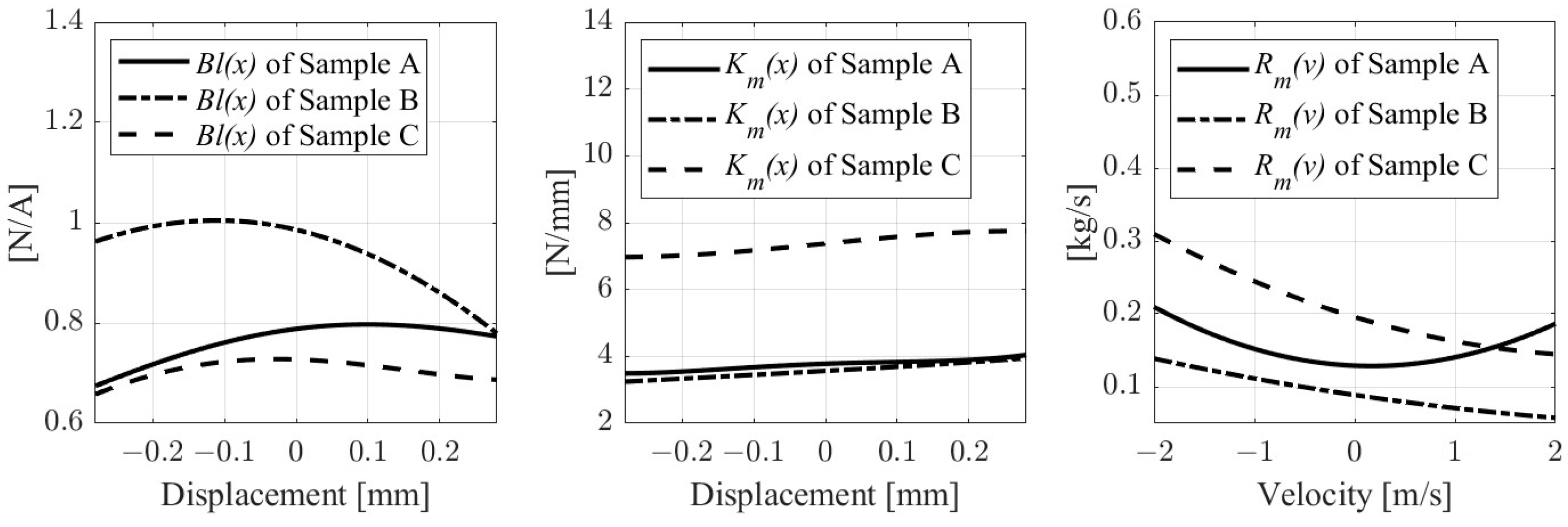
The sample parameters used for the theoretical calculations were obtained from measurements using a Klippel R&D LPM system. The linear parameters Re, Le, and Mm were measured using the Klippel LPM module. These measurements also provided linear displacement data, which were used to derive K2 and R2 by fitting with a theoretical model, as reported in Ref. [16]. Notably, K2 and R2 were obtained under linear conditions and used for computation and prediction within the nonlinear model. The rationale for this approach is discussed in the subsequent section. The measured and fitted linear parameters of the three samples are presented in Table 1. The nonlinear parameters Bl, Km, and Rm were measured using the Klippel LSI module, and the results are shown in Figure 3.

Table 1.
Linear parameters of the samples.

Figure 3.
Nonlinear parameters of samples.
Subsequently, the displacement waveforms were predicted using the state–space equations from the two models, as described in Section 2.3. The THD values were then predicted using Equation (14).
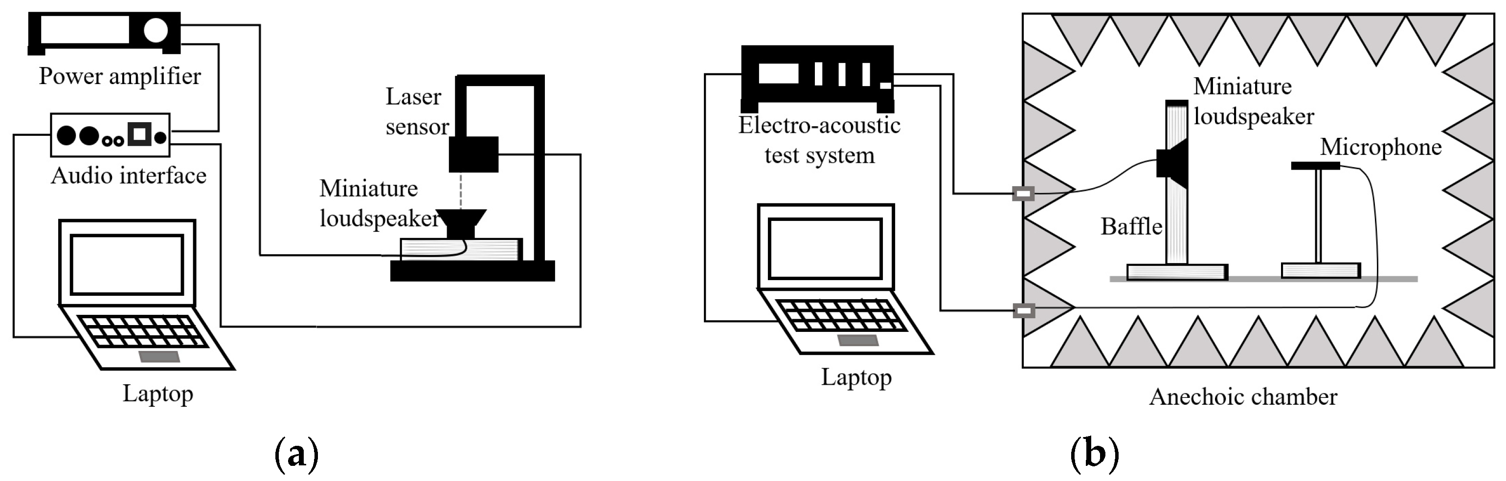
The displacement waveforms and THD values under nonlinear conditions were measured as shown in Figure 4. The experimental setup for displacement measurement is depicted in Figure 4a. During the experiments, the samples were mounted on a laser measurement platform, with signal transmission and reception controlled by a laptop via an audio interface (Fireface UC, RME, Haimhausen, Germany). Two music clips containing rich low-frequency components were chosen as input signals, considering the dominant domain of the creep effect. Clip 01 was from the song “Hotel California” by the band The Eagles from their album “Hotel California”. Clip 02 came from the song “The Ferry” by the singer Tsai Chin featured on the album “Folk Songs by Tsai Chin”. These tracks are often used in audio assessments of low-frequency and dynamic performance. Each clip was excerpted to 30 s and sampled at 48 kHz. The root-mean-square (RMS) value of the input voltage was set at 2 V. The excitation signal was generated by the interface and delivered to the samples through a power amplifier (RMX 2450, QSC, Costa Mesa, CA, USA). Concurrently, the displacement signal was recorded using a laser probe (LK-G30, KEYENCE, Osaka, Japan) and fed back into the audio interface. This facilitated the acquisition of the displacement waveforms.
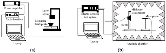
Figure 4.
Setup for the experimental measurements of (a) displacement and (b) sound pressure level (SPL) and THD.
The THD values of the miniature loudspeaker samples were evaluated in an anechoic chamber (5.8 m × 4.8 m × 2.9 m). As illustrated in Figure 4b, the samples were mounted on a baffle for the experimental procedures. The RMS value of the stepped sine input voltage was set at 2 V, and the frequency range was adjusted to 30–4000 Hz to ensure that the THD was evaluated across a broad frequency domain. A reference microphone (SCM-3, Listen Inc., Boston, MA, USA) was positioned 5 cm in front of the samples to capture the sound pressure signal under far-field conditions. The sound pressure signals were measured and analyzed using SoundCheck software 14.01 and the corresponding hardware interface for audio measurement (AmpConnect ISC, Listen Inc., Boston, MA, USA).
3.2. Results and Discussion
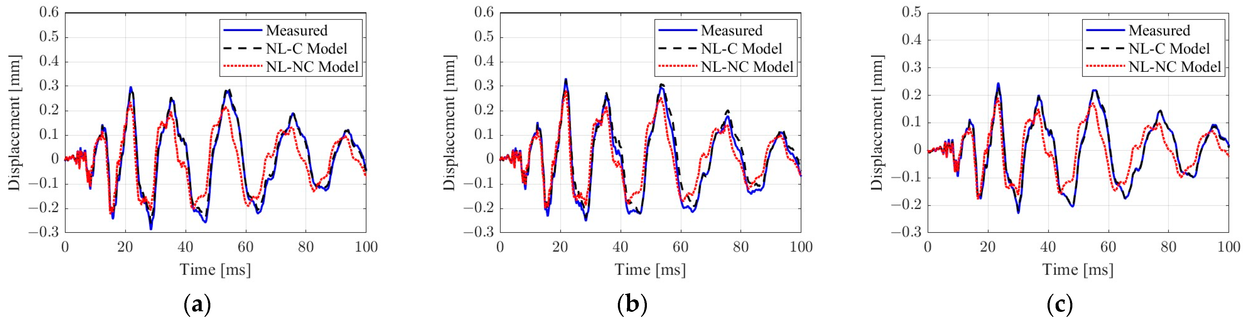
The predicted and experimental displacement waveforms of the three samples are illustrated in Figure 5. The displacement waveforms predicted by the NL-C model align more closely with the measurement values than the NL-NC model, confirming that the NL-C model better reproduces the electrical dynamics of the miniature loudspeakers. This is primarily because music signals contain rich low-frequency components, leading to a prominent creep effect. The NL-NC model does not account for creep, causing discrepancies between the predicted and measured displacement waveforms.
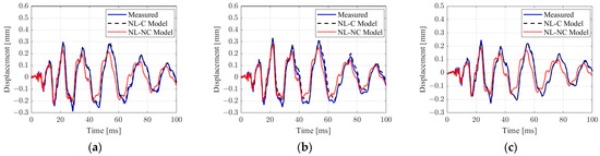
Figure 5.
Comparison of the predicted and measured displacement waveforms for Clip 01: (a) sample A, (b) sample B, and (c) sample C. A 100 ms window was selected to display the differences in waveforms. The stimulus length was 30 s.
The root-mean-square error (RMSE) is a key quantitative indicator used to assess the average magnitude of the errors between predicted values and measured values. RMSE is defined as follows:
where x represents the data under evaluation, N represents the numbers of data points, and the subscripts m and p indicate the measured and predicted values, respectively. The magnitude of RMSE is indicative of the discrepancy between the predicted and measured data. A lower RMSE value signifies a higher model accuracy and a closer alignment between the predicted and measured values.
Table 2 displays the RMSE values for the displacement waveforms predicted using the two models across various frequency ranges. Overall, the NL-C model demonstrated better accuracy than the NL-NC model in both the low- and full-frequency ranges. In the low-frequency domain, where the disparity in RMSE between the two models was most pronounced, the NL-C model significantly outperformed the NL-NC model. However, in the high-frequency range, there was no noticeable difference in accuracy between the two models because the creep effect is negligible in this range. Thus, the NL-C model is more representative of actual loudspeaker behavior because it accounts for the creep effect, particularly at low frequencies.
Table 2.
The RMSE values for nonlinear displacement waveforms.
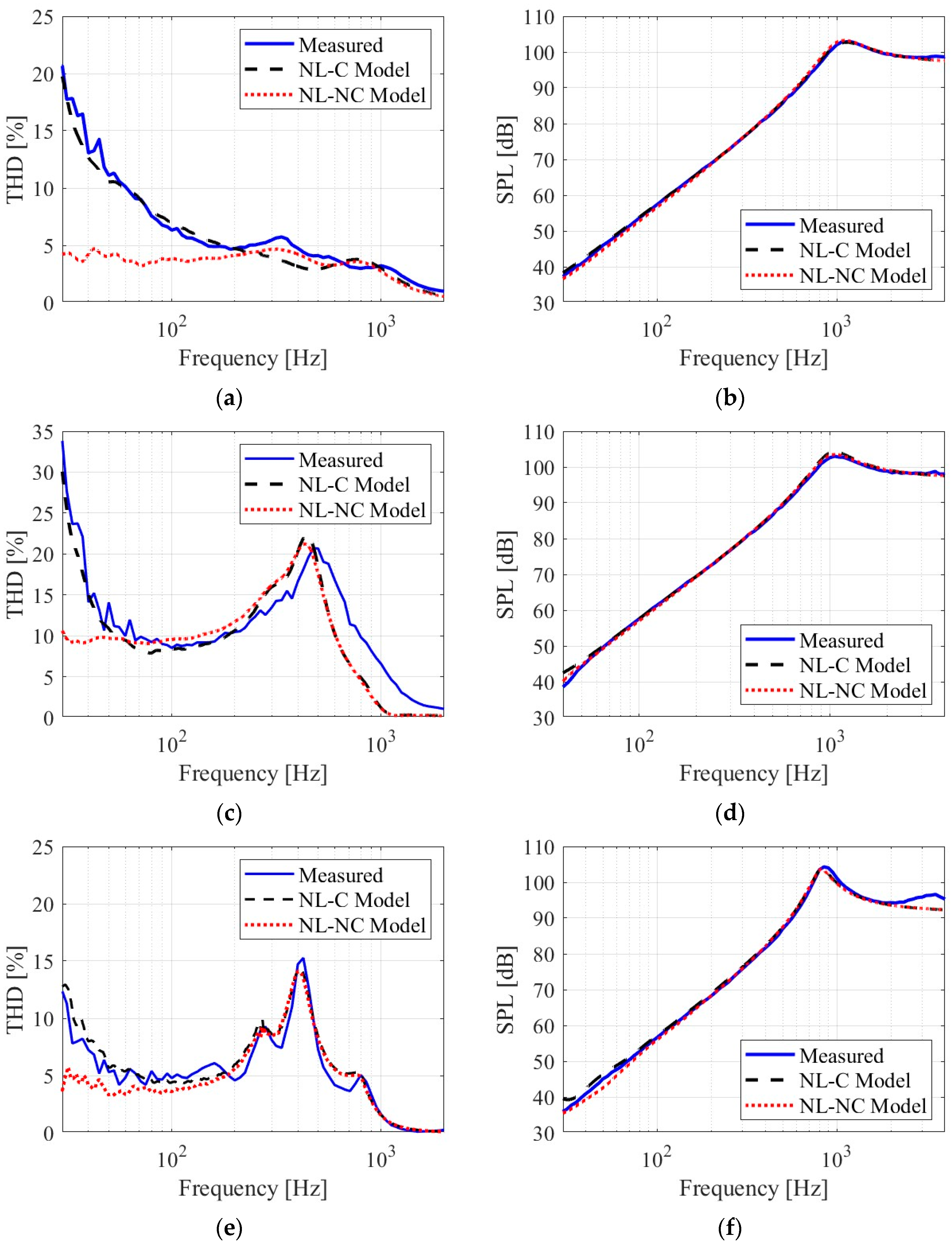
The predicted and measured THD and sound pressure level (SPL) values of the three samples are compared in Figure 6. The THD values predicted by both models were relatively consistent for all samples at frequencies beyond 500 Hz. However, at low frequencies, particularly those below 200 Hz, noticeable disparities emerged between the measured THD values and those predicted by the NL-NC model. The NL-NC model was inadequate for forecasting the substantial distortions observed at low frequencies. In contrast, the THD values predicted by the NL-C model corresponded well with the measurement values in nearly the entire frequency domain. In contrast to THD, the disparities in SPL were minimal, even at low frequencies. This can be attributed to the frequency response of the loudspeakers, which conforms to a high-pass model that results in minimal output at low frequencies. As a result, the variations caused by the creep effect are mitigated. Consequently, the differences in the predicted and measured SPL values were negligible for both models.
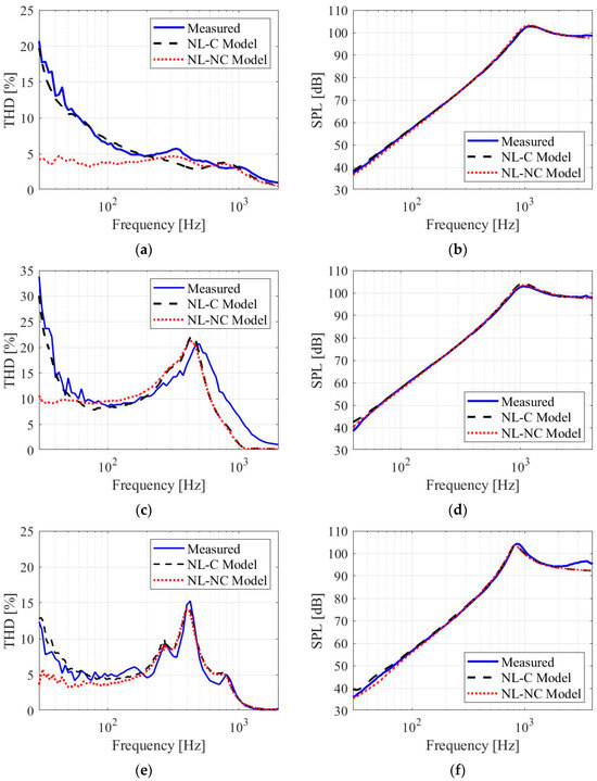
Figure 6.
Comparison of the measured and predicted THD and SPL values: (a) THD of sample A, (b) SPL of sample A, (c) THD of sample B, (d) SPL of sample B, (e) THD of sample C, and (f) SPL of sample C.
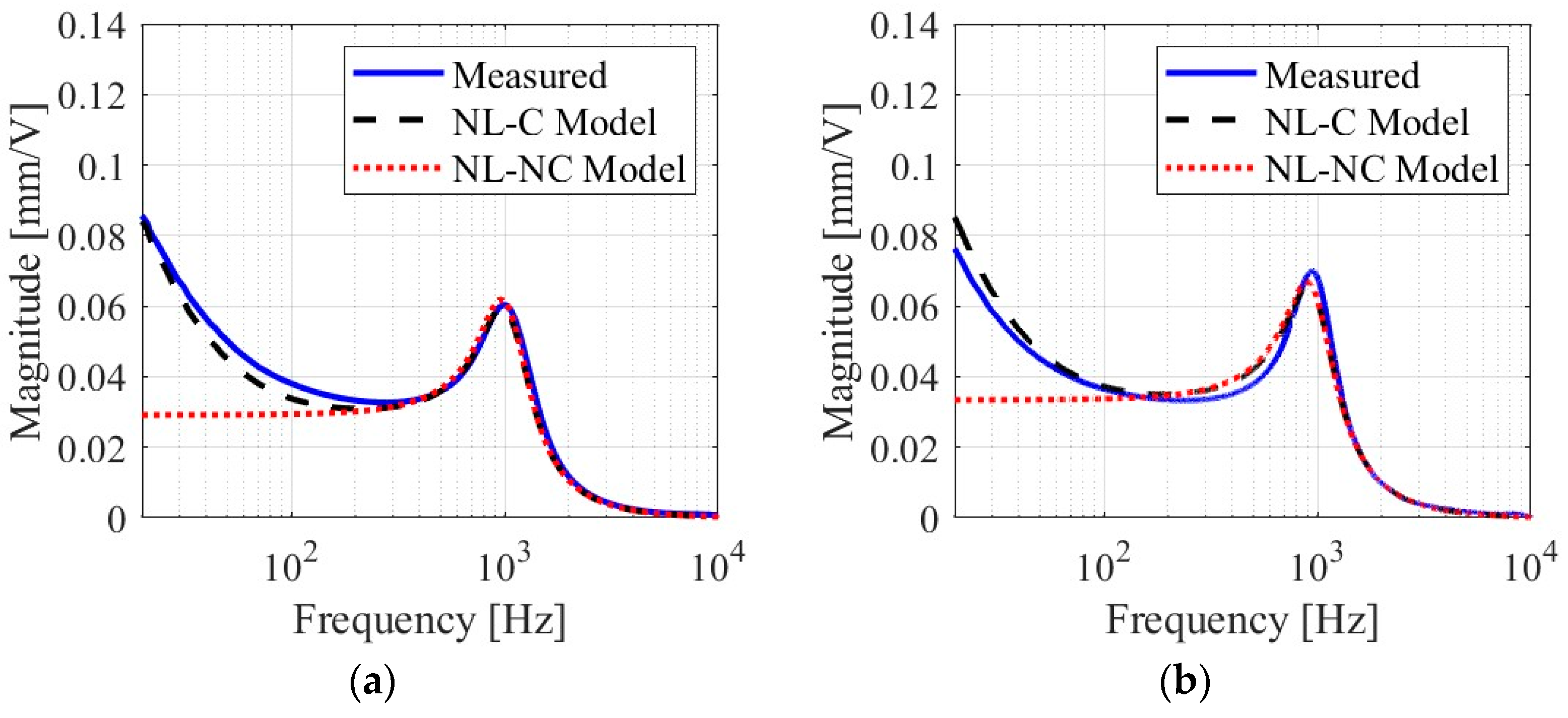
In the experiments mentioned above, the secondary parameters K2 and R2 for creep were determined by the small-signal displacement data measured under linear conditions. To verify the appropriateness of these parameters for the nonlinear model, the displacement transfer function curves were measured and predicted under both linear and nonlinear conditions, taking sample A as an example (Figure 7). The measurement data shown in Figure 7a were acquired at an RMS voltage of 0.2 V to ensure the sample remained in a linear state. In contrast, the measurement data shown in Figure 7b were obtained under an RMS voltage of 2 V to ensure the sample was in a nonlinear state. The theoretical predictions under both conditions were made using the same values of K2 and R2. The predictions of the NL-C model in Figure 7a were expected to align more closely with the actual measurement data since the creep parameters were derived from the linear measurement data. Due to the model’s limitations, within the frequency range of 40–200 Hz, the predicted displacements were slightly lower than the actual measurements. Comparing the nonlinear displacement transfer function curves in Figure 7b shows that the curve predicted by the NL-C model is consistently more accurate than the one predicted by the NL-NC model. At frequencies below 50 Hz, the predictions of the NL-C model exceeded the actual measurements, and deviations were also observed in the middle frequency range of 200–1000 Hz. In summary, the predictions of the NL-C model were still markedly superior to those of the NL-NC model. Considering the data shown in Figure 7 and the previous comparisons of the predicted and measured displacement waveforms, the method used for rapidly estimating creep parameters from linear displacement data is acceptable for practical applications.
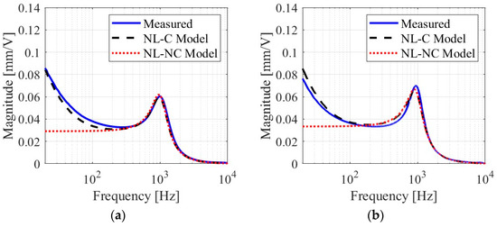
Figure 7.
Comparison of the predicted and measured displacement transfer functions for sample A under (a) linear and (b) nonlinear conditions.
4. Conclusions
This paper presents a nonlinear model for miniature loudspeakers in consideration of the creep effect. This model improves upon the traditional NL-NC model by conserving the creep effect caused by the loudspeaker suspension when evaluating the nonlinear performance. The creep effect is modeled as a combination of linear springs and viscous dashpots in reference to the theory of linear viscoelastic mechanics. The validity of the new NL-C model was confirmed by comparison with the experimental data. The displacements and THD values predicted by the NL-C model agreed well with the measurement values, especially in the low-frequency range. The results also confirmed that the creep effect plays a significant role in low-frequency displacement in miniature loudspeakers, with substantial low-frequency distortions generated by the enhancement of low-frequency displacements.
The two key conclusions of this study are as follows. First, in comparison with the NL-NC model, the NL-C model is a more effective time domain method for the prediction of nonlinear displacement and THD in miniature loudspeakers, particularly within the low-frequency range. Second, the creep effect significantly enhances low-frequency displacement, which markedly increases harmonic distortions in the same frequency band. The NL-C model can be applied in future investigations of displacement and distortion compensation in miniature loudspeakers.
Author Contributions
Conceptualization, S.C. and J.H.; methodology, S.C.; software, S.C. and J.H.; validation, S.C. and F.S.; formal analysis, S.C. and F.S.; data curation, S.C.; writing—original draft preparation, S.C.; writing—review and editing, J.H., X.F. and Y.S; supervision, X.F. and Y.S.; project administration, X.F. and Y.S.; funding acquisition, Y.S. All authors have read and agreed to the published version of the manuscript.
Funding
This work was supported by the National Natural Science Foundation of China (Grant No. 12374446).
Institutional Review Board Statement
Not applicable.
Informed Consent Statement
Not applicable.
Data Availability Statement
The data presented in this study are available on request from the corresponding author. The data are not publicly available due to privacy.
Conflicts of Interest
The authors declare no conflict of interest.
References
- Frank, W.; Reger, R.; Appel, U. Loudspeaker nonlinearities-analysis and compensation. In Proceedings of the Twenty-Sixth Asilomar Conference on Signals, Systems & Computers, Pacific Grove, CA, USA, 26–28 October 1992. [Google Scholar]
- Klippel, W. Adaptive nonlinear control of loudspeaker systems. J. Audio Eng. Soc. 1998, 46, 939–954. [Google Scholar]
- Quaegebeur, N.; Chaigne, A. Nonlinear vibrations of loudspeaker-like structures. J. Sound Vib. 2008, 309, 178–196. [Google Scholar] [CrossRef]
- Merit, B.; Lemarquand, V.; Lemarquand, G.; Dobrucki, A. Motor nonlinearities in electrodynamic loudspeakers: Modelling and measurement. Arch. Acoust. 2009, 34, 579–590. [Google Scholar]
- Klippel, W. Nonlinear large-signal behavior of electrodynamic loudspeakers at low frequencies. J. Audio Eng. Soc. 1992, 40, 483–496. [Google Scholar]
- Klippel, W. Tutorial: Loudspeaker nonlinearities—Causes, parameters, symptoms. J. Audio Eng. Soc. 2006, 54, 907–939. [Google Scholar]
- Dobrucki, A. Nontypical effects in an electrodynamic loudspeaker with a nonhomogeneous magnetic field in the air gap and nonlinear suspensions. J. Audio Eng. Soc. 1994, 42, 565–576. [Google Scholar]
- Bai, M.R.; Huang, C.M. Expert diagnostic system for moving-coil loudspeakers using nonlinear modeling. J. Acoust. Soc. Am. 2009, 125, 819–830. [Google Scholar] [CrossRef] [PubMed]
- Roylance, D. Engineering Viscoelasticity; Department of Materials Science and Engineering, Massachusetts Institute of Technology: Cambridge, MA, USA, 2001; Volume 2139, pp. 1–37. [Google Scholar]
- Knudsen, M.H.; Hansen, P.; Jensen, J.G. The significance of viscoelastic effects in loudspeakers parameter measurements. In Proceedings of the 88th Convention of the Audio Engineering Society, New York, NY, USA, 13–16 March 1990. [Google Scholar]
- Knudsen, M.H.; Jensen, J.G. Low-frequency loudspeaker models that include suspension creep. J. Audio Eng. Soc. 1993, 41, 3–18. [Google Scholar]
- Seidel, U. Fast and accurate measurement of the linear transducer parameters. In Proceedings of the 110th Convention of the Audio Engineering Society, New York, NY, USA, 12–15 May 2001. [Google Scholar]
- Agerkvist, F.T.; Ritter, T. Modeling viscoelasticity of loudspeaker suspensions using retardation spectra. In Proceedings of the 129th Convention of the Audio Engineering Society, New York, NY, USA, 4–7 November 2010. [Google Scholar]
- Hiebel, H. Suspension creep models for miniature loudspeakers. In Proceedings of the 132nd Convention of the Audio Engineering Society, Budapest, Hungary, 26–29 April 2012. [Google Scholar]
- Findley, W.N.; Davis, F.A. Creep and Relaxation of Nonlinear Viscoelastic Materials; Courier Corporation: North Chelmsford, MA, USA, 2013; pp. 52–58. [Google Scholar]
- Agerkvist, F.; Thorborg, K.; Tinggard, C. A study of the creep effect in loudspeaker suspension. In Proceedings of the 125th Convention of the Audio Engineering Society, San Francisco, CA, USA, 2–5 October 2008. [Google Scholar]
- Petošić, A.; Đurek, I.; Đurek, D. Modeling of an electrodynamic loudspeaker including membrane viscoelasticy. In Proceedings of the 124th Convention of the Audio Engineering Society, New York, NY, USA, 17–20 May 2008. [Google Scholar]
- Thorborg, K.; Tinggaard, C.; Agerkvist, F.; Futtrup, C. Frequency dependence of damping and compliance in loudspeaker suspensions. J. Audio Eng. Soc. 2010, 58, 472–486. [Google Scholar]
- Falaize, A.; Hélie, T. Passive modelling of the electrodynamic loudspeaker: From the Thiele–Small model to nonlinear port-Hamiltonian systems. Acta Acust. 2020, 4, 1. [Google Scholar] [CrossRef]
- Brosch, R. Loudspeaker Simulation considering Suspension Creep. Master’s Thesis, Institute of Signal Processing and Speech Communication, Graz University of Technology, Graz, Austria, 2020. [Google Scholar]
- King, A.; Agerkvist, F. Fractional derivative loudspeaker models for nonlinear suspensions and voice coils. J. Audio Eng. Soc. 2018, 66, 525–536. [Google Scholar] [CrossRef]
- Tian, X.; Shen, Y.; Chen, L.; Zhang, Z. Identification of nonlinear fractional derivative loudspeaker model. J. Audio Eng. Soc. 2020, 68, 355–363. [Google Scholar] [CrossRef]
Disclaimer/Publisher’s Note: The statements, opinions and data contained in all publications are solely those of the individual author(s) and contributor(s) and not of MDPI and/or the editor(s). MDPI and/or the editor(s) disclaim responsibility for any injury to people or property resulting from any ideas, methods, instructions or products referred to in the content. |
© 2024 by the authors. Licensee MDPI, Basel, Switzerland. This article is an open access article distributed under the terms and conditions of the Creative Commons Attribution (CC BY) license (https://creativecommons.org/licenses/by/4.0/).