Article

Study on the Optical Coupling Effect of Building-Integrated Photovoltaic Modules Applied with a Shingled Technology

Department of Electrical and Computer Engineering, Sungkyunkwan University, Suwon 16419, Republic of Korea
*
Author to whom correspondence should be addressed.
Appl. Sci. 2024, 14(13), 5759; https://doi.org/10.3390/app14135759
Submission received: 21 May 2024 / Revised: 26 June 2024 / Accepted: 27 June 2024 / Published: 1 July 2024

Abstract

:
Building-integrated photovoltaics (BIPV) comprise the integration of a solar power generation system into the exterior design and architectural elements of a building to produce electricity, which allows the building itself to generate electricity. By integrating shingled technology into the photovoltaic module with optimization of the optical effect, the output performance of the module can be increased while securing an aesthetic appeal as an architectural exterior material for the building simultaneously. In this research, we studied enhancing the performance of BIPV modules through an analysis of the optical coupling effect for shingled technology using PSpice simulation. Compared to the efficiency of 0.2 cm string spacing, the optical coupling effect was increased by 33.33%, 46.98%, 67.01%, and 193.49% according to the string spacing of 0.5 cm, 1 cm, 2 cm and 4 cm, respectively. To analyze this increase, we focused on studying the increase in current due to the reflection and re-absorption of light in the back layer of the solar cell as the cause of this output enhancement. Additionally, the coupling effect in accord with different layers showed that using white EVA to reflect the incident light from the top layer resulted in 117.14% and 521.90% enhancements in maximum output power (Pm) loss % compared to the conventional and black backsheet applied PV modules, respectively.

1. Introduction

To achieve carbon neutrality by replacing or absorbing emissions in response to global warming, there is growing interest in solar power generation [1,2,3,4,5]. Solar power generation is a method of producing electricity from solar panels using sunlight. It does not require fuel because it produces electricity from the sun and does not emit harmful substances into the atmosphere during the generation process [6,7]. Additionally, solar power generation is nearly silent during the electricity generation process and has minimal impact on the surrounding environment during construction, making it increasingly popular as an environmentally friendly energy source [8,9,10]. Recently, the importance of BIPV power generation significantly increased due to various demands on energy usage in densely populated areas with buildings [11,12]. BIPV integrates a solar power generation system into the architectural exterior elements of a building to allow the building itself to produce electricity [13,14,15]. It can be installed in various locations, such as windows, exterior walls, roofs, and more, and is like a building material that can generate its own electricity rather than a separate solar power facility. Because BIPV does not require a separate site, it can be harmoniously integrated into the design of buildings, which makes it easy for residents to accept. By integrating solar modules into buildings, BIPV enables buildings to generate their own electricity, reducing their reliance on grid power, which can lead to energy offsets and contribute to reducing electricity peaks during high and low seasons [16,17,18]. This environmentally friendly solar energy technology can increase the added value of buildings and can be applied to both new construction and existing building renovations [19,20]. However, there are obstacles to the adoption of BIPV, such as high initial installation cost, technical complexity, sustainability of the market and economic feasibility. Especially, since BIPV modules are installed on a limited area of the building, the power generation capacity is relatively low, which ultimately results in low efficiency compared with initial cost [21,22,23]. The shingled technology was proposed to address these issues by connecting cells with electrically conductive adhesives (ECA) to increase cell density and consequently enhance module output [24]. However, the impact of the spacing between shingled strings on output variation has not been thoroughly studied. Understanding the key factors for maximizing the development efficiency of building-integrated photovoltaics (BIPV) is crucial. so, it is important to understand the key factor for maximizing power generation of BIPV. In this study, the performance enhancement of a BIPV module was studied through the optical coupling effect of the shingled PV module using PSpice simulation. To verify simulation results, BIPV modules were fabricated by using four shingled strings, with each string made up of 17 interconnected divided cells were large enough to allow an analysis of the changes in factors. For the comparative analysis based on spacing between strings, modules were fabricated with string spacing of 0.2 cm, 0.5 cm, 1 cm, 2 cm, and 4 cm, and the coupling effect under each condition was analyzed. In addition, the coupling effect on the module performance according to the reflection of light was studied by analyzing the optical coupling effect based on the different interlayers of the module.

2. Materials and Methods

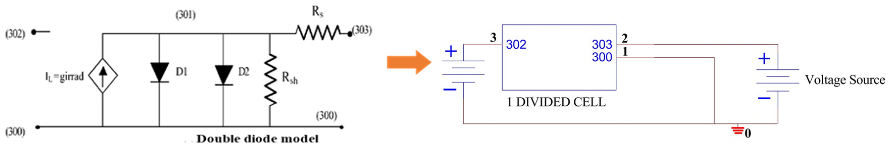
2.1. Shingled Module Circuit Modeling

A recently highlighted method for manufacturing PV modules is the shingled technology to enhance the output power of the module by fabricating a shingled structure of solar cells called a shingled string. This method involves cutting solar cells with a laser, connecting the divided cells in series using electrically conductive adhesives (ECA) to make a shingled string, then arranging strings to fabricate a PV module. The advantage of this method is that it allows an increase in the number of cells and the active area of the module by removal of spaces between solar cells, resulting in a higher output. In addition, it provides a more attractive exterior because there is no visible circuitry on it, and strings can be manufactured in various sizes depending on the installation location, so, it can serve as an aesthetically pleasing building cladding material [24,25,26]. Because of these characteristics, PV modules can be effective in generating power in areas with limited installation space, especially for the BIPV [27].
Before fabricating the shingled BIPV module, PSpice simulation was carried out first to predict the change in output value based on the spacing between strings through a simulation model. Figure 1 shows the schematic of the double diode model and a divided cell circuit diagram for the PSpice simulation.
For the simulation, divided cells were measured with a solar simulator (WXA-155S-L2, WACOM, Kazo, Japan) and modeled using a double diode model. Figure 2 shows the schematic illustration of a shingled string and module modeling.
Seventeen divided solar cells were interconnected in series to make one shingled string, and a total of four strings were used to fabricate a module. Also, the resistance component was applied to each string to reflect the series resistance from the ECA for interconnecting the 17 divided solar cells.

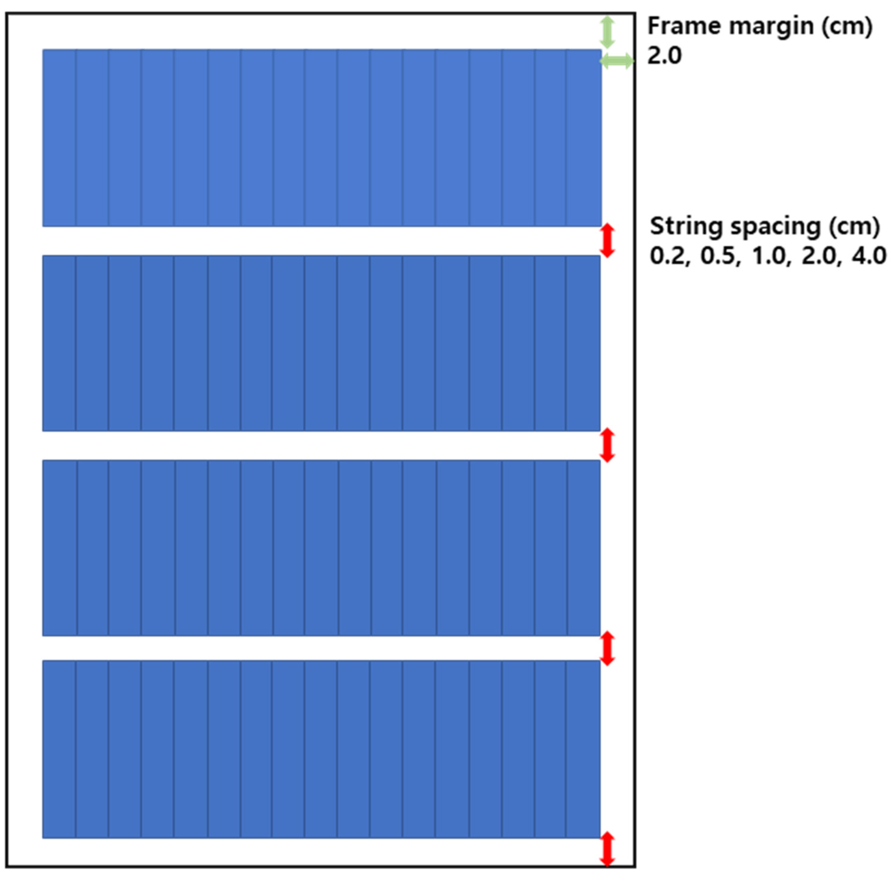
2.2. Preparation of Shingled Strings

The production process for a shingled BIPV module consisted of three main stages: the singulation process of dividing cells, the cell–string connection process for serially connecting the divided cells to form a string, and the module assembly process [28,29]. For the singulation, multi-crystalline solar cells, p-type, 6 inch, 5 busbars, 20.2% conversion efficiency, were used to fabricate shingled strings. A 532 nm green laser (Coherent, Santa Clara, CA, USA) was used for laser scribing along the busbar on solar cells (scan speed 1300 mm/s, frequency 50 kHz, repetition number 30 times), and scribed cells were mechanically broken for separation. The cell–string interconnection process involves dispensing ECA on the front busbar of the divided cell and bonding it to the rear Ag pad of the neighboring divided cell with an overlap width of 1.4 mm. A total of 17 divided cells were used for each string, and after dispensing ECA, the string was heated to 150 °C for 5 s on a hot plate for ECA curing.

2.3. Preparation of Shingled BIPV Modules

Each prepared string was arranged in a series-parallel configuration and encapsulated through the module manufacturing process to create a shingled photovoltaic module, as shown in Figure 3.
To analyze the optical coupling effect according to the string distance between strings, white ethylene vinyl acetate (EVA) was used for the bottom of the encapsulating layer, and 5 modules were manufactured with string spacing of 0.2 cm, 0.5 cm, 1 cm, 2 cm, and 4 cm, respectively, while the frame margin was fixed at a distance of 2.0 cm as shown in Figure 4.
In addition, to compare the performance between the white EVA module used and a conventional module, a BIPV module using a UV-transparent EVA was manufactured as shown in Figure 5.
To accurately determine the output characteristics of the modules, factors that could affect the output were kept constant. All modules were made of four strings, and each string consisted of 17 divided cells connected by ECA with a 0.14 cm overlap width. For comparison between a conventional module and the module using white EVA, the string spacing was fixed at 0.5 cm.

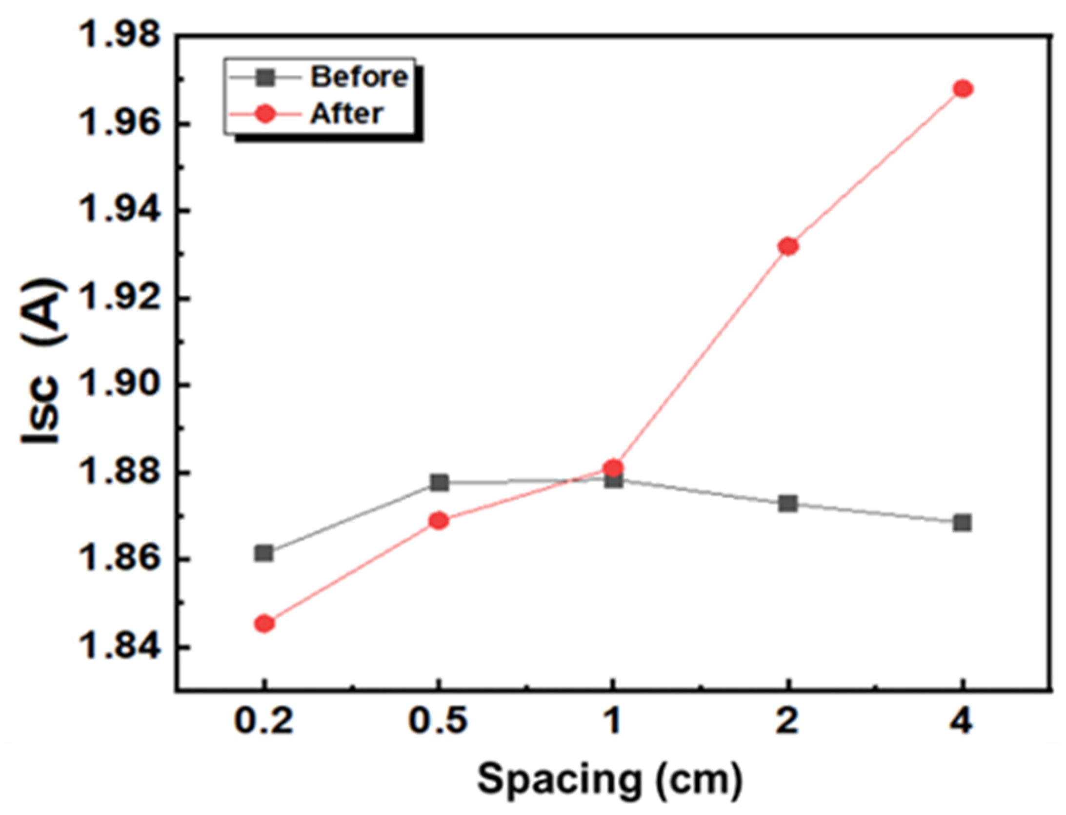
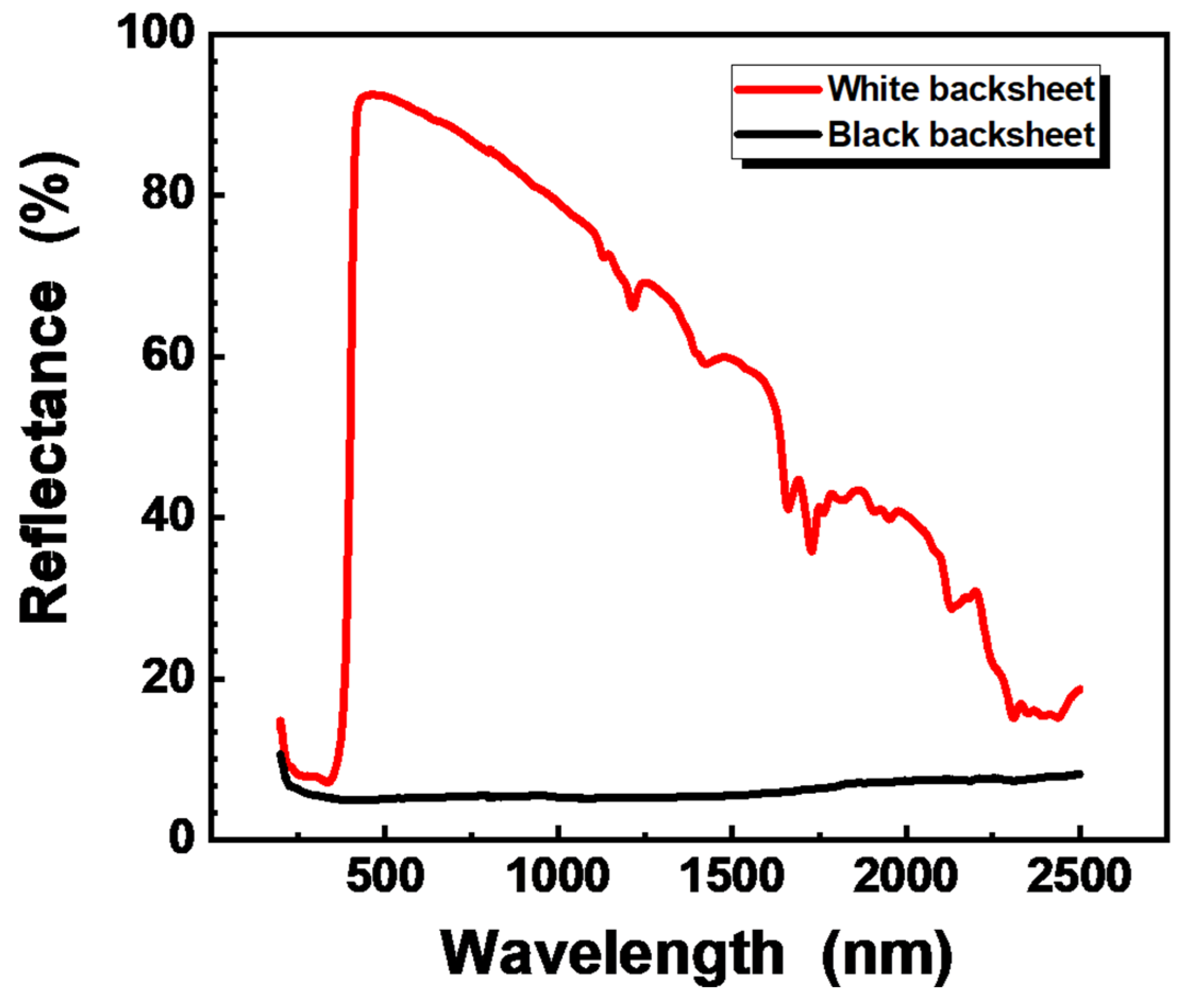
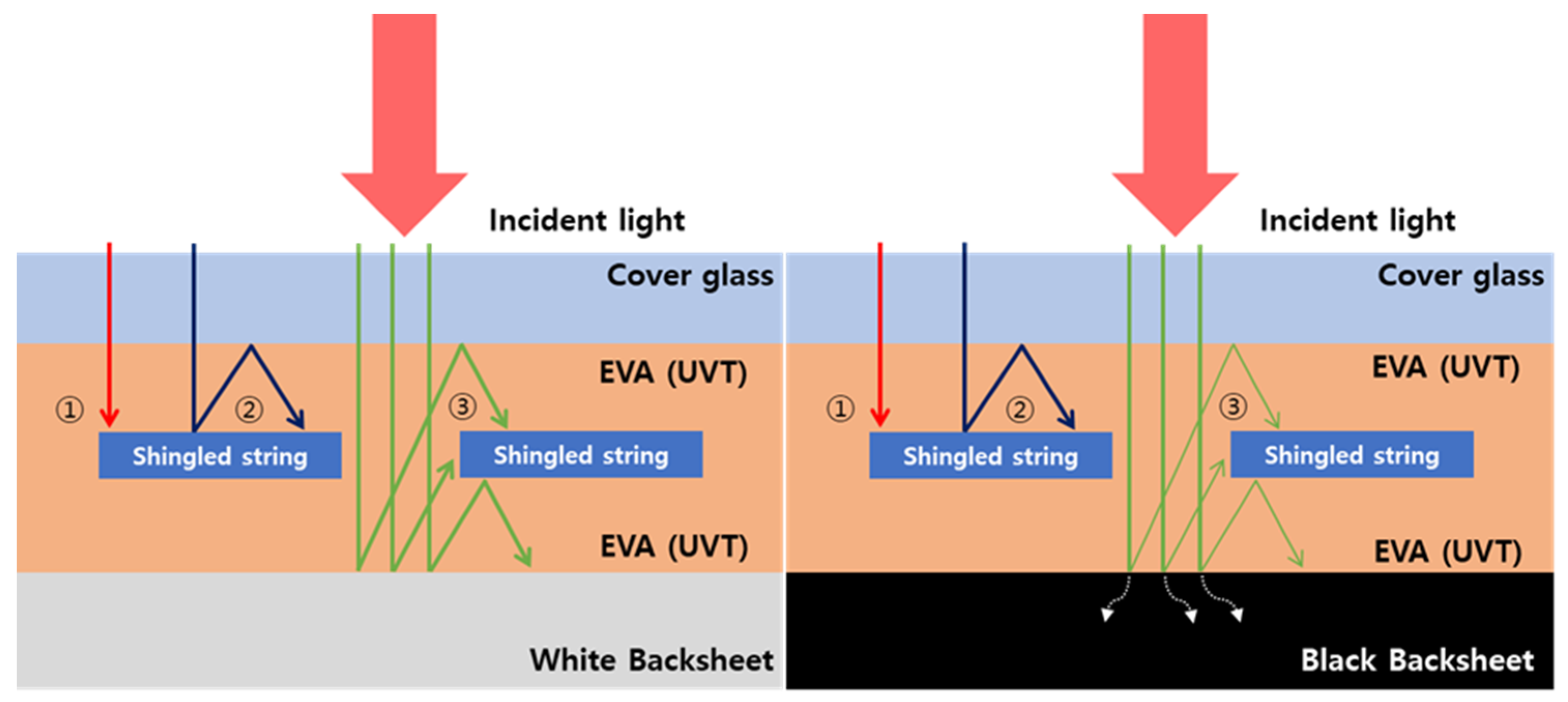
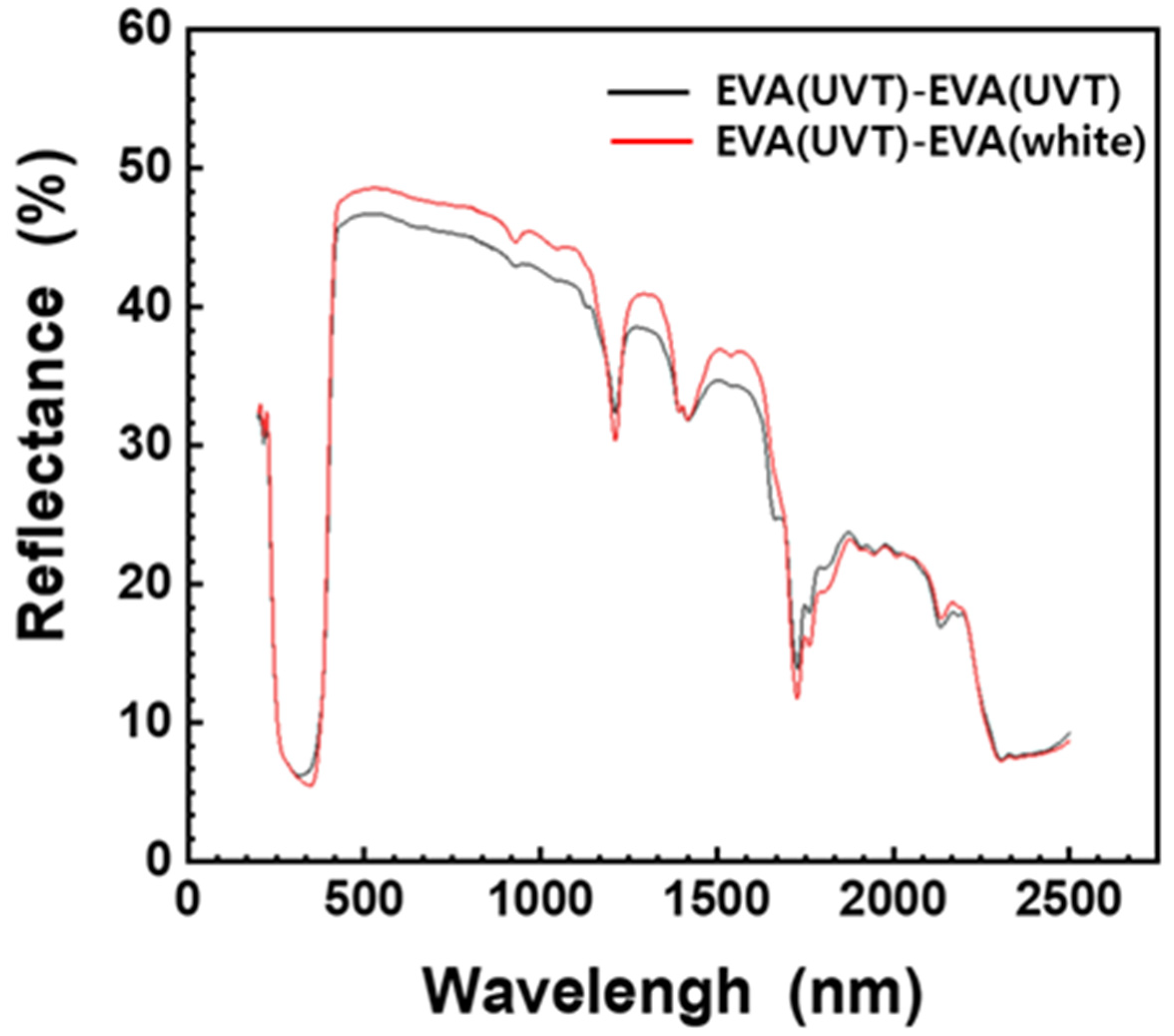
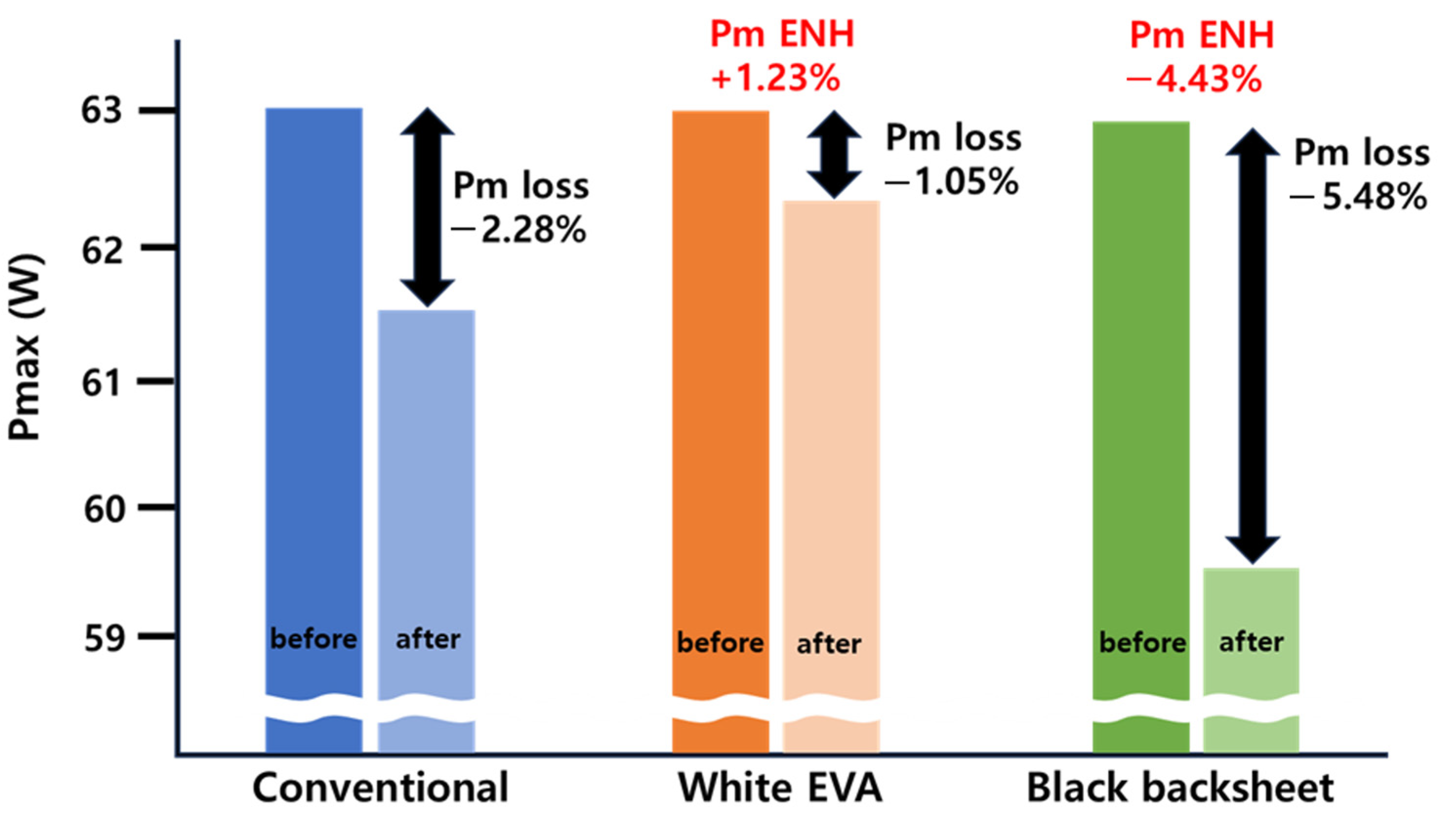
3. Results and Discussion

To protect solar cells from outer environmental conditions, they are encapsulated for protection and retaining the stability of the solar cells, but the encapsulation process causes optical loss [30]. When incident light arrives at the PV module, some is absorbed, transmitted and reflected at each layer of the module. Optical losses are primarily classified by reflection loss at interfaces and absorption loss at each layer. Due to the optical losses occurring as light passes through each medium, there is an inevitable loss known as cell-to-module (CTM) loss when assembling solar cells into modules [31,32,33]. Figure 6 shows the path of incident light and the optical coupling effect inside a module. As it shows, reflection loss occurs at the interfaces of air–glass, glass–encapsulant, encapsulant–white backsheet, as well as the surface of the solar cells, but at the same time, some light is reflected to the solar cells again and induces optical gain. Typically, a material with high reflectance is used for the backsheet; some fraction of the light reflected by the backsheet is absorbed by the solar cells owing to the optical coupling effect, and the amount of reflected light depends on the spacing between solar cells. As the spacing increases, more light is reflected, and the chance of absorption by solar cells also increases, while decreased spacing results in the opposite effect. Therefore, the balance between the spacing of the cells and the amount of reflected light is very important to minimize the CTM loss and maximize the performance of the BIPV modules [34].
To investigate changes in optical characteristics of the shingled strings based on the spacing, different spacings of strings were modeled for the simulation using PSpice. Table 1 shows the simulated results for strings with different spacings, and clearly, the results show a correlation between the spacing and Pm. As the spacing increased, Pm also increased because of more reflected light from the spacing.
To verify the simulation results, real solar modules were fabricated for comparison. By analyzing the solar cell string output before and after lamination with changes in string spacing, we could determine how the optical coupling effect of different string spacings affects the output values before and after lamination. The typical structure of a solar module consists of a cover glass, EVA, solar cells, EVA, and a backsheet; in each layer, light transmission and reflection occur. Table 2 shows the measured results before and after lamination of a string with 0.2 cm spacing.
On average, there was an efficiency loss of approximately 0.6% for each string, and the open-circuit voltage decreased by approximately 0.95% for all strings, whereas Isc decreased by an average of 1.5%. Table 3 lists the output characteristics of the strings with 0.5 cm spacing. At a spacing of 0.5 cm, there was a decrease of approximately 1.0% in open-circuit voltage characteristics, similarly to the 0.2 cm spacing. However, as the spacing increased to 0.5 cm, the shunt current loss decreased. The shunt current losses were on average 0.2%, which is a decrease of 1.3% compared with the 0.2 cm spacing. As a result, the overall efficiency decreased by an average of 0.448%.
Table 4 shows the output characteristics of the string. At spacing of 1 cm, the shunt current showed higher values than before lamination. The shunt current increased by 0.3% compared with before lamination. The efficiency decreased by an average of 0.28%.
At a spacing of 2 cm, the efficiency of the laminated string increased compared with that of the non-laminated string, as shown in Table 5. After lamination, the string exhibited a 0.29% efficiency increase. On average, the shunt current of each string increased by 2.9%, and the open-circuit voltage exhibited characteristics similar to those of the previous string spacing. In the case of 4 cm spacing, Table 6, the highest efficiency increase was observed. The efficiency increased by 0.58%, and the shunt current increased by approximately 5%.
Overall, as the string spacing increased, the short-circuit current increased accordingly. The change in average power output before and after lamination decreased by −0.485 W at a 0.2 cm string spacing, −0.323 W at 0.5 cm, and −0.257 W at 1 cm, but increased by 0.185 W at 2 cm and 0.453 W at 4 cm. Typically, due to cell-to-module (CTM) losses that occur when solar cells are modularized, the output should decrease. However, in this case, the power output of the solar cells increased after the lamination process. The rate of increase in output after the lamination process, based on the 0.2 cm spacing, was 33.33% at 0.5 cm, 46.98% at 1 cm, 67.01% at 2 cm, and 193.49% at 4 cm. Figure 7 shows the short-circuit current values according to string spacing. When the laminated string spacing became longer than 0.5 cm, short-circuit current values were increased compared with non-laminated strings. In the case of efficiency, as shown in Figure 8, overall efficiency was increased when laminated string spacing became longer than 1 cm.
One of the representative methods to increase the efficiency of a photovoltaic module is to optimize the spacing between strings so that the reflected light can be reabsorbed by the solar cells. The wider the spacing, the more light is reflected from the rear and reabsorbed, generating more electron–hole pairs and resulting in a higher current. As shown in Figure 7, the amount of Isc increases as the spacing between strings increases. This increase in Isc leads to improved string efficiency, which in turn results in higher module efficiency. However, increasing the spacing between strings in the same area also decreases the number of solar cells that can be installed, leading to a decrease in the module’s active area and consequently its efficiency. Considering this trade-off, it is evident that optimal string spacing is required to maximize module performance. Future research will focus on determining the optimal string spacing that balances increased light reabsorption and the number of solar cells, ensuring the best possible output for photovoltaic modules.
In the previous experiments, the output characteristics of a string were analyzed based on the spacing between strings. To analyze the optical coupling effect of the material that reflects the light entering the module, three modules with the same structure, excluding the backsheet and EVA, were fabricated, and their output characteristics were analyzed. For the experiment, 20.2% Multi PERC cells and four shingled strings of 17 interconnected cells with a 0.14 cm overlap width and 0.5 cm string spacing were prepared as described in the previous experiment. Figure 9 shows the structure of the three modules with partially different layers. The experiment was conducted using a cover glass/ultraviolet transparent (UVT) EVA/string/EVA (UVT)/white backsheet configuration, as well as configurations with cover glass/EVA/string/EVA (white)/white backsheet and cover glass/EVA (UVT)/string/EVA (UVT)/black backsheet.
Table 7 lists the measured characteristics before and after the lamination of the shingled string with a white backsheet, which is commonly used in typical solar modules. As shown in the table, the efficiency of the string decreased by an average of 0.448% after lamination, despite the efficiency increase owing to reflection in the white backsheet.
Table 8 lists the measured characteristics before and after the lamination of the shingled string with a black backsheet. Black backsheets are commonly used in shingled solar modules to unify the color of the shingled strings and enhance their aesthetics. However, it is difficult to expect reflection from the rear because of the application of black color in the rear. As shown in the results, an average efficiency loss of 1.07% occurred after lamination. This loss is significantly higher than that observed for a typical white backsheet, which exhibits an efficiency loss of 0.6%. Figure 10 shows the reflectance measurements of white and black backsheets. As illustrated in the figure, the black backsheet has a significantly lower reflectance, resulting in a total efficiency loss of 1.07%. In contrast, fabricating the module with a white backsheet can improve efficiency by approximately 0.6%.
Table 9 lists the results obtained by applying white EVA instead of the commonly used UV-transparent EVA.
EVA to the module. As shown in the results, the module with white EVA showed a decrease in efficiency of approximately 0.2% after lamination. However, owing to the increase in reflection from the backside compared with the conventional structure, the short-circuit current increased about 1%, and the efficiency increased about 0.24% after lamination.
Figure 11 shows a cross-sectional view of the module with EVA (UVT) applied and the module with EVA (white) applied.
As shown in the left figure, in a typical module structure, the incident light is not only reflected at the top of the string but also at the spacing between strings, and part of the reflected light is directed towards the back of the solar cell. However, in the module with white EVA, more reflected light was absorbed by the string owing to the optical coupling effect, and was reflected on the white backsheet with a strong reflection coefficient for the spacing between strings. Compared with a typical module, there is no reflection component from the backsheet to the rear surface of the string. Instead, more light reflected from the white backsheet located between strings is absorbed into the strings. Consequently, the amount of light absorbed by the strings owing to the coupling effect increases, resulting in a higher output than that of a typical module. Figure 12 shows the reflectance according to the wavelength of the conventional EVA (UVT)—EVA (UVT)—white backsheet (left) and EVA (UVT)—EVA (UVT)—black backsheet (right) modules. Because of the absorption at the black backsheet, less light is reflected, and the overall performance of the module consequently decreased.
As shown in Figure 13, the modules with white EVA exhibited higher reflectivity in the 400–1100 nm range than a typical module, and more reflected light was absorbed by the strings, leading to an increase in the module output. Figure 14 and Table 10 show Pm loss comparisons before and after the lamination process between the conventional EVA (UVT)—EVA (UVT)—white backsheet structure, EVA (UVT)—EVA (white)—white backsheet structure, and EVA (UVT)—EVA (UVT)—black backsheet structure. As the graph shows, the module with white EVA applied had an additional Pm of 4.43% from the rear reflection compared with the black module. Also, compared with the conventional module, a white EVA module resulted in an additional Pm increase of 1.23%.

4. Conclusions

In this study, the optical coupling effect dependent on the string spacing in the shingled module was studied by simulation and comparative analysis of the fabricated module. The efficiency of the module increased as the spacing between strings increased because of the enhanced optical coupling effect. For modules with string spacings of 0.2 cm, 0.5 cm and 1 cm, the efficiencies decreased by 3.07%, 2.05% and 1.63%, respectively, after the lamination of the strings. In contrast, when the string spacing was 2 cm, the efficiency increased by 1.18%, and when it was 4 cm, the efficiency increased by 2.87%. Based on the efficiency of 0.2 cm spacing, the optical coupling effect according to the string spacing was increased by 33.33%, 46.98, 67.01%, and 193.49% for spacings of 0.5 cm, 1 cm, 2 cm, and 4 cm, respectively. Furthermore, the coupling effect according to the structure of the different layers showed that using white EVA to reflect the incident light from the top layer resulted in an enhanced Pm loss 117.14% higher than that of using a UV-transparent EVA, which can be considered to increase the output of the module. Through our research, we have demonstrated that the amount of light reflected from the rear and reabsorbed by the module varies depending on the spacing between strings and the types of module material. However, increasing the spacing between strings in the same area has the advantage of enhancing string efficiency due to the increased reabsorption of light from the rear, but it also has the drawback of reducing the number of solar cells that can be installed in the module, leading to a decrease in overall performance. Therefore, to achieve the best performance, it is necessary to optimize the string spacing considering the area of the photovoltaic module. This optimization will be addressed in more detail in future research. As a result of the research, it is possible to explore ways to improve the output power of BIPV modules installed in limited spaces. Also, it is expected that the results can contribute to energy efficiency in buildings by enhancing the performance of BIPV modules.

Author Contributions

Conceptualization, J.L.; methodology, S.U. and J.K.; formal analysis, H.J.; investigation, S.U. and J.K.; writing—original draft preparation, H.J., J.K. and S.U.; writing—review and editing, J.L.; visualization, J.K. and S.U.; supervision, J.L. All authors have read and agreed to the published version of the manuscript.

Funding

This work was supported by the Human Resources Development of the Korea Institute of Energy Technology Evaluation and Planning (KETEP) grant funded by the Korea government Ministry of Trade, Industry and Energy (No. RS-2023-00266248). Also, the authors acknowledge the financial support of the Korean Institute of Energy Technology Evaluation and Planning (KETEP) and the Ministry of Trade, Industry and Energy (MOTIE) of the Republic of Korea (No. 20213030010290).

Institutional Review Board Statement

Not applicable.

Informed Consent Statement

Not applicable.

Data Availability Statement

The data that support the findings of this study are available upon reasonable request.

Conflicts of Interest

The authors declare no conflicts of interest.

References

  1. Armstrong McKay, D.I.; Staal, A.; Abrams, J.F.; Winkelmann, R.; Sakschewski, B.; Loriani, S.; Fetzer, I.; Cornell, S.E.; Rockström, J.; Lenton, T.M. Exceeding 1.5 °C global warming could trigger multiple climate tipping points. Science 2022, 377, 6611. [Google Scholar] [CrossRef] [PubMed]
  2. Wang, F.; Harindintwali, J.D.; Yuan, Z.; Wang, M.; Wang, F.; Li, S.; Yin, Z.; Huang, L.; Fu, Y.; Li, L.; et al. Technologies and perspectives for achieving carbon neutrality. Innovation 2021, 2, 100180. [Google Scholar] [CrossRef] [PubMed]
  3. Liu, Z.; Deng, Z.; He, G.; Wang, H.; Zhang, X.; Lin, J.; Qi, Y.; Liang, X. Challenges and opportunities for carbon neutrality in China. Nat. Rev. Earth Environ. 2022, 3, 141–155. [Google Scholar] [CrossRef]
  4. Lenton, T.M.; Held, H.; Kriegler, E.; Hall, J.W.; Lucht, W.; Rahmstorf, S.; Schellnhuber, H.J. Tipping elements in the Earth’s climate system. Proc. Natl. Acad. Sci. USA 2008, 6, 1786–1793. [Google Scholar] [CrossRef] [PubMed]
  5. Lenton, T.M.; Rockström, J.; Gaffney, O.; Rahmstorf, S.; Richardson, K.; Steffen, W.; Schellnhuber, H.J. Climate tipping points-too risky to bet against. Nature 2019, 575, 592–595. [Google Scholar] [CrossRef]
  6. Singh, G.K. Solar power generation by PV (photovoltaic) technology: A review. Energy 2013, 53, 1–13. [Google Scholar] [CrossRef]
  7. Ahmadi, M.H.; Ghazvini, M.; Sadeghzadeh, M.; Alhuyi Nazari, M.; Kumar, R.; Naeimi, A.; Ming, T. Solar power technology for electricity generation: A critical review. Energy Sci. Eng. 2018, 6, 340–361. [Google Scholar] [CrossRef]
  8. Urbina, A. The balance between efficiency, stability and environmental impacts in perovskite solar cells: A review. J. Phys. Energy 2020, 2, 022001. [Google Scholar] [CrossRef]
  9. Miles, R.; Hynes, K.; Forbes, I. Photovoltaic solar cells: An overview of state-of-the-art cell development and environmental issues. Prog. Cryst. 2005, 51, 1–42. [Google Scholar] [CrossRef]
  10. Serrano-Lujan, L.; Espinosa, N.; Larsen-Olsen, T.T.; Abad, J.; Urbina, A.; Krebs, F.C. Tin- and Lead ased Perovskite Solar Cells under Scrutiny: An Environmental Perspective. Adv. Energy Mater. 2015, 5, 1501119. [Google Scholar] [CrossRef]
  11. Shukla, A.K.; Sudhakar, K.; Baredar, P. Recent advancement in BIPV product technologies: A review. Energy Build. 2017, 150, 188–195. [Google Scholar] [CrossRef]
  12. Biyik, E.; Araz, M.; Hepbasli, A.; Shahrestani, M.; Yao, R.; Shao, L.; Essah, E.; Oliveira, A.C.; del Caño, T.; Rico, E.; et al. A key review of building integrated photovoltaic (BIPV) systems. Eng. Sci. Technol. Int. J. 2017, 20, 833–858. [Google Scholar] [CrossRef]
  13. Kuhn, T.E.; Erban, C.; Heinrich, M.; Eisenlohr, J.; Ensslen, F.; Neuhaus, D.H. Review of techno-logical design options for building integrated photovoltaics (BIPV). Energy Build. 2021, 231, 110381. [Google Scholar] [CrossRef]
  14. Henemann, A. BIPV: Built-in solar energy, Renew. Energy Focus 2008, 9, 14–19. [Google Scholar] [CrossRef]
  15. Yang, R.J. Building integrated photovoltaics (BIPV): Costs, benefits, risks, barriers and improvement strategy. Int. J. Constr. Manag. 2016, 16, 39–53. [Google Scholar] [CrossRef]
  16. Shukla, A.K.; Baredar, P.; Mamat, R.; Sudhakar, K. BIPV in Southeast Asian countries–opportunities and challenges. Renew. Energy Focus 2017, 21, 25–32. [Google Scholar] [CrossRef]
  17. Kamel, R.S.; Fung, A.S. Modeling, simulation and feasibility analysis of residential BIPV/T+ASHP system in cold climate—Canada. Energy Build. 2014, 82, 758–770. [Google Scholar] [CrossRef]
  18. Do, S.L.; Shin, M.; Baltazar, J.; Kim, J. Energy benefits from semi-transparent BIPV window and daylight-dimming systems for IECC code-compliance residential buildings in hot and humid climates. Sol. Energy 2017, 155, 291–303. [Google Scholar] [CrossRef]
  19. Saretta, E.; Caputo, P.; Frontini, F. A review study about energy renovation of building facades with BIPV in urban environment. Energy Sustain. Soc. 2019, 44, 343–355. [Google Scholar] [CrossRef]
  20. Aguacil, S.; Lufkin, S.; Rey, E. Active surfaces selection method for building-integrated photovoltaics (BIPV) in renovation projects based on self-consumption and self-sufficiency. Energy Build. 2019, 193, 15–28. [Google Scholar] [CrossRef]
  21. Lee, H.M.; Yoon, J.H. Power performance analysis of a transparent DSSC BIPV window based on 2 year measurement data in a full-scale mock-up. Appl. Energy 2018, 225, 1013–1021. [Google Scholar] [CrossRef]
  22. Liu, B.; Duan, S.; Cai, T. Photovoltaic DC-Building-Module-Based BIPV System—Concept and Design Considerations. IEEE Trans. Power Electron. 2011, 26, 1418–1429. [Google Scholar] [CrossRef]
  23. Song, J.H.; An, Y.S.; Kim, S.G.; Lee, S.J.; Choung, Y.K.; Yoon, J.H. Power output analysis of transparent thin-film module in building integrated photovoltaic system (BIPV). Energy Build. 2008, 40, 2067–2075. [Google Scholar] [CrossRef]
  24. Jee, H.; Song, J.; Moon, D.; Lee, J.; Jeong, C. Improvement in power of shingled solar cells for photo-voltaic module. J. Nanosci. Nanotechnol. 2020, 20, 7096–7099. [Google Scholar] [CrossRef] [PubMed]
  25. Oh, W.; Jee, H.; Bae, J.; Lee, J. Busbar-free electrode patterns of crystalline silicon solar cells for high density shingled photovoltaic module. Sol. Energy Mater. Sol. Cells 2022, 243, 111802. [Google Scholar] [CrossRef]
  26. Oh, W.; Park, J.; Dimitrijev, S.; Kim, E.K.; Park, Y.S.; Lee, J. Metallization of crystalline silicon solar cells for shingled photovoltaic module application. Sol. Energy 2020, 195, 527–535. [Google Scholar] [CrossRef]
  27. Ravyts, S.; Vecchia, M.D.; Broeck, G.V.; Yordanov, G.H.; Goncalves, J.E.; Moschner, J.D.; Saelens, D.; Driesen, J. Embedded BIPV module-level DC/DC converters: Classification of optimal ratings. Renew. Energy 2020, 146, 880–889. [Google Scholar] [CrossRef]
  28. Oh, W.; Park, J.; Jeong, C.; Park, J.; Yi, J.; Lee, J. Design of a solar cell electrode for a shingled photovoltaic module application. Appl. Surf. Sci. 2020, 510, 145420. [Google Scholar] [CrossRef]
  29. Schulte-Huxel, H.; Blankemeyer, S.; Morlier, A.; Brendel, R.; Koentges, M. Interconnect-shingling: Maximizing the active module area with conventional module processes. Sol. Energy Mater. Sol. Cells 2019, 200, 109991. [Google Scholar] [CrossRef]
  30. Shen, L.; Li, Z.; Ma, T. Analysis of the power loss and quantification of the energy distribution in PV module. Appl. Energy 2020, 260, 114333. [Google Scholar] [CrossRef]
  31. Roy, J.N. Comprehensive analysis and modeling of cell to module (CTM) conversion loss during c-Si Solar Photovoltaic (SPV) module manufacturing. Sol. Energy 2016, 130, 184–192. [Google Scholar] [CrossRef]
  32. Bermudez, V.; Perez-Rodriguez, A. Understanding the cell-to-module efficiency gap in Cu(In,Ga)(S,Se)2 photovoltaics scale-up. Nat. Energy 2018, 3, 466–475. [Google Scholar] [CrossRef]
  33. Jung, T.H.; Lee, J.I.; Song, H.E.; Ju, Y.C.; Ko, S.W.; Jung, Y.S.; Kang, G.H. Classification conditions of cells to reduce cell-to-module conversion loss at the production stage of PV modules. Renew. Energy 2017, 103, 582–593. [Google Scholar] [CrossRef]
  34. Yousuf, H.; Zahid, M.A.; Khokhar, M.Q.; Park, J.; Ju, M.; Lim, D.; Kim, Y.; Cho, E.-C.; Yi, J. Cell-to-Module Simulation Analysis for Optimizing the Efficiency and Power of the Photovoltaic Module. Energies 2022, 15, 1176. [Google Scholar] [CrossRef]
Figure 1. A double diode model and a divided cell circuit diagram.
Applsci 14 05759 g001
Figure 2. The schematic illustration of a shingled string and module modeling.
Applsci 14 05759 g002
Figure 3. Shingled BIPV module with white EVA.
Applsci 14 05759 g003
Figure 4. Top view of the shingled module (with the frame margin fixed at 2.0 cm, indicated by the green arrow, and the string spacing varied between 0.2 and 4.0 cm, indicated by the red arrow).
Applsci 14 05759 g004
Figure 5. Conventional structure of a shingled BIPV module.
Applsci 14 05759 g005
Figure 6. Path of incident light and the optical coupling effect within a PV module (reflection at the interfaces of (1) air–cover glass, (2) cover glass–encapsulant, (3) surface of the solar cells, (4) encapsulant–white backsheet, (5) encapsulant–cover glass).
Applsci 14 05759 g006
Figure 7. Short-circuit current vs. spacing between strings (◼ before lamination, after lamination).
Applsci 14 05759 g007
Figure 8. Efficiency changes according to spacing between strings.
Applsci 14 05759 g008
Figure 9. Shingled BIPV modules with three different types of backsheet. Top: conventional EVA (UVT) -EVA (UVT)—white backsheet structure; middle: EVA (UVT)—EVA (white)—white backsheet structure; bottom: EVA (UVT)—EVA (UVT)—black backsheet structure.
Applsci 14 05759 g009
Figure 10. Reflectance according to the wavelength of the white backsheet and the black backsheet.
Applsci 14 05759 g010
Figure 11. Cross-sectional view of the module with EVA (UVT)—EVA (UVT) applied (left) and the module with EVA (UVT)—EVA (white) applied (right).
Applsci 14 05759 g011
Figure 12. Cross-sectional view of the module with EVA (UVT)—EVA (UVT)—white backsheet (left) and EVA (UVT)—EVA (UVT)—black backsheet (right) modules.
Applsci 14 05759 g012
Figure 13. Reflectance according to the wavelength of the EVA (UVT)—EVA (UVT) applied (black graph) and the module with EVA (UVT)—EVA (white) (red graph).
Applsci 14 05759 g013
Figure 14. Output power loss comparison of before and after lamination process between the conventional EVA (UVT)—EVA (UVT)—white backsheet structure (left), EVA (UVT)—EVA (white)—white backsheet structure (center), and EVA (UVT)—EVA (UVT)—black backsheet structure (right).
Applsci 14 05759 g014
Table 1. Simulated results for strings with different spacings.
Before LaminationAfter Lamination
Spacing
[cm]
Isc
[A]
Voc
[V]
FF
[%]
Eff
[%]
Pm
[W]
Isc
[A]
Voc
[V]
FF
[%]
Eff
[%]
Pm
[W]
0.21.8311.1277.4119.6815.751.7911.1177.419.2315.39
0.51.8311.1277.4819.7015.761.8111.1177.5119.4815.59
11.8311.1277.5119.7115.771.8211.1277.4119.5615.66
21.8711.1377.6420.1216.101.8311.1277.4819.7015.77
41.9011.1477.7220.5516.451.8311.1277.5719.7315.79
Definition: Isc: Short-circuit current, Voc: Open-circuit voltage, FF: Fill factor, Eff: Efficiency, Pm: Maximum output.
Table 2. Output characteristics of fabricated module based on the spacing between shingled strings (spacing 0.2 cm).
Before LaminationAfter Lamination
Spacing
[cm]
String No.Isc
[A]
Voc
[V]
FF
[%]
Eff
[%]
String No.Isc
[A]
Voc
[V]
FF
[%]
Eff
[%]
0.211.88211.13275.319.70311.83811.02774.818.947
21.88011.13875.519.74721.84911.03675.019.138
31.86211.12775.919.64731.84511.01675.019.045
41.87311.11775.719.70741.85111.01275.519.222
Table 3. Output characteristics of fabricated module based on the spacing between shingled strings (spacing 0.5 cm).
Before LaminationAfter Lamination
Spacing
[cm]
String No.Isc
[A]
Voc
[V]
FF
[%]
Eff
[%]
String No.Isc
[A]
Voc
[V]
FF
[%]
Eff
[%]
0.551.87211.14075.619.70451.87311.03474.719.294
61.87311.11775.519.6561.86410.99974.919.188
71.87811.12475.619.73971.86910.99474.819.215
81.87311.13375.819.74581.87511.00975.019.347
Table 4. Output characteristics of fabricated module based on the spacing between shingled strings (spacing 1.0 cm).
Before LaminationAfter Lamination
Spacing
[cm]
String No.Isc
[A]
Voc
[V]
FF
[%]
Eff
[%]
String No.Isc
[A]
Voc
[V]
FF
[%]
Eff
[%]
1.091.87411.11975.719.71391.87711.01975.419.488
101.86911.11975.719.667101.87911.01975.019.41
111.87811.1375.219.652111.88111.0374.619.343
121.86811.14375.719.696121.87711.02574.919.363
Table 5. Output characteristics of fabricated module based on the spacing between shingled strings (spacing 2.0 cm).
Before LaminationAfter Lamination
Spacing
[cm]
String No.Isc
[A]
Voc
[V]
FF
[%]
Eff
[%]
String No.Isc
[A]
Voc
[V]
FF
[%]
Eff
[%]
2.0 cm131.87611.12475.519.683131.93111.03674.819.915
141.88211.1375.519.762141.92811.0575.119.988
151.87311.12375.619.68151.93211.03374.619.872
161.87511.12375.519.686161.93311.03774.719.918
Table 6. Output characteristics of fabricated module based on the spacing between shingled strings (spacing 4.0 cm).
Before LaminationAfter Lamination
Spacing
[cm]
String No.Isc
[A]
Voc
[V]
FF
[%]
Eff
[%]
String No.Isc
[A]
Voc
[V]
FF
[%]
Eff
[%]
4.0 cm171.87611.1375.419.68171.97611.03774.720.347
181.88111.15475.419.766181.9711.07874.520.319
191.86911.14976.019.773191.96811.05674.620.296
201.87411.12975.619.691201.96411.04774.820.27
Table 7. Measured string characteristics of a shingled module with white backsheet (before and after lamination).
String No.Pm [W]Isc [A]Voc [V]FF [%]Eff [%]
Before lamination115.7691.87211.13975.619.704
215.7251.87311.11775.519.649
315.7971.87811.12375.619.739
415.8011.87311.13275.819.744
After lamination115.4401.87311.03374.719.293
215.3551.86410.99974.919.187
315.3771.86910.99474.819.215
415.4831.87511.00975.019.347
Table 8. Measured string characteristics of a shingled module with black backsheet (before and after lamination).
String No.Pm [W]Isc [A]Voc [V]FF [%]Eff [%]
Before lamination515.7341.87011.12275.719.661
615.7251.87511.11975.419.649
715.7241.87411.13875.319.648
815.8011.87311.13275.819.744
After lamination514.8781.74510.99477.618.591
614.8941.75210.99477.318.611
714.8951.75711.01277.018.612
814.8641.76010.98776.918.574
Table 9. Measured string characteristics of a shingled module with white EVA (before and after lamination).
String No.Pm [W]Isc [A]Voc [V]FF [%]Eff [%]
Before lamination915.7851.88011.14475.319.724
1015.7161.86611.11475.819.638
1115.7771.86311.13476.119.714
1215.7881.87711.12375.619.728
After lamination915.5651.91311.03674.919.449
1015.5851.87711.02875.319.474
1115.6171.88011.02775.319.514
1215.6381.88911.01975.119.540
Table 10. Performance comparison between the conventional EVA (UVT) —EVA (UVT)—white backsheet structure, EVA (UVT)—EVA (white)—white backsheet structure, EVA (UVT)—EVA (UVT)—black backsheet structure.
TypePm Before Lamination (W)Pm After Lamination (W)Pm Loss (%)Enhanced Pm Loss of White EVA vs. UVT EVA, Black Backsheet Structure (%)
UVT EVA63.09261.6552.28117.14
White EVA63.06662.4051.05-
Black backsheet62.98459.5315.48521.90
Disclaimer/Publisher’s Note: The statements, opinions and data contained in all publications are solely those of the individual author(s) and contributor(s) and not of MDPI and/or the editor(s). MDPI and/or the editor(s) disclaim responsibility for any injury to people or property resulting from any ideas, methods, instructions or products referred to in the content.

