Analysis and Experiment of Thermal Field Distribution and Thermal Deformation of Nut Rotary Ball Screw Transmission Mechanism

Abstract

This study designs a differential dual-drive micro-feed mechanism, superposing the two “macro feed motions” (“motor drive screw” and “motor drive nut”) using the same transmission of “the nut rotary ball screw pair” structure. These two motions are almost equal in terms of speed and turning direction, thus the “micro feed” can be obtained. (1) Background: Thermal deformation is the primary factor that can restrict the high-precision micro-feed mechanism and the distribution of heat sources differs from that of the conventional screw single-drive system owing to the structure and motion features of the transmission components. (2) Discussion: This study explores the thermal field distribution and thermal deformation of the differentially driven micro-feed mechanism when two driving motors are combined at different speeds. (3) Methods: Based on the theory of heat transfer, the differential dual-drive system can be used as the research object. The thermal equilibrium equations of the micro-feed transmission system are established using the thermal resistance network method, and a thermal field distribution model is obtained. (4) Results: Combined with the mechanism of thermal deformation theory, the established thermal field model is used to predict the axial thermal deformation of the differential dual-drive ball screw. (5) Conclusions: Under the dual-drive condition, the steady-state thermal error of the nut-rotating ball screw transmission mechanism increases with the increase in nut speed and composite speed and is greater than the steady-state thermal error under the single screw drive condition. After reaching the thermal steady state, the measured thermal elongation at the end of the screw in the experiment is approximately 10.5 μm and the simulation result is 11.98 μm. The experimental measurement result demonstrates the accuracy of the theoretical analysis model for thermal error at the end of the screw.

1. Introduction

Ultra-precision machining technology is an important research direction in the manufacturing equipment industry and is a fundamental technology for the development of cutting-edge technologies, the national defense industry, aviation, aerospace, microelectronics, optics, biology, medicine, and genetic engineering [1,2]. It is also a key technology that determines a country’s comprehensive strength and international status. For most precision and ultra-precision optical instruments, scanning probe microscopes, semiconductor technology equipment, microelectromechanical system (MEMS) detection, and micro/nano machining machines, the thermal error is an important factor affecting the feed accuracy of the system, which can reduce the geometric and machining accuracy of the machine tool [3,4]. The thermal deformation error resulting from heat accounts for 40–70% of the total error of the machine tool [5]. The temperature rise and thermal deformation of the screw nut are caused by the relative motion friction and heat generation between the contact parts, and they are the primary heat sources of the system. Moreover, the thermal error of the screw, particularly the axial thermal error, makes a significant impact on the final machining accuracy. Therefore, investigating the temperature field distribution of the system and the variation law of axial thermal error of the ball screw becomes a vital direction for enhancing the transmission accuracy of the feed system.

The research results obtained using the thermal resistance network method include the following representative articles: Han L [6] established a temperature-distribution-related thermal resistance network model based on the thermal resistance network as well as the spherical wall heat conduction principle to improve the thermal design of the chip package structure. Li DT [7] proposed a new simulation approach according to the thermal resistance network approach and the chamber model, with the consideration of impacts of heat exchange, leakage, and component deformation and temperature. Sun ZH [8] presented a lumped-parameter thermal resistance network model for a permanent-magnet spherical motor to track its temperature transients. Meng QY [9] proposed thermal contact resistance (TCR) between contact surfaces and established the motorized spindle mathematical model by incorporating different fractal parameters. Zhu ZY [10] proposed an equivalent thermal resistance network approach for evaluating the temperature increase in an axial permanent-magnet magnetic bearingless flywheel machine, and they established an equivalent thermal network model based on the theory of baseline heat transfer. Bao YJ [11] developed a composite material thermal resistance network model by incorporating heat transfer direction and fiber ply angle based on a series–parallel resistance computing approach. In addition, they described their results, which were determined through thermal response tests for unidirectional carbon fiber laminates. Zhan ZQ [12] developed an implicit thermal network method for the accurate and efficient calculation of temperature, which mainly focused on converting the observed time-varying variables that served as the heat source and thermal resistance to latent variables to construct an implicit thermal equilibrium equation. To obtain real-time dynamic characteristics of ball bearings, Li TJ [13] presented a new model for calculating point-contact dynamic friction within blended lubrication, and they established a time-varying thermal contact resistance model to fit between the ball and the ring, between the housing and the ring, and between the shaft and the ring based on heat transfer and fractal theories. Yang YB [14] proposed a computationally volumetric heat source model according to a semi-analytical thermal modeling method, which was applied in modeling the thermal response during a selective laser melting process.

The following representative articles examine the feed system’s temperature field distribution. Wu HY [15] derived a positive temperature field for ideal heat source heat transfer as well as a heat-transfer-induced negative temperature field by examining the heat transfer of a ball screw and the heat generation mechanism; they also established a dynamic temperature field mathematical model for the ball screw feed system with regard to position and time in line with the temperature field superposition principle. Liu JL [16] proposed an approach for optimizing thermal boundary conditions, such as thermal loads, thermal contact resistance, and the convective heat transfer coefficient, thus improving the accuracy of the conventional transient thermal characteristics analysis model in simulating the ball screw feed drive system. Sheng X [17] developed an analytical method for solving the temperature field distribution within a finite cylinder body resulting from periodic-motion heat sources and constant strength and proposed two heat source models, namely multiple and single. Taking a 250 kW permanent-magnet governor that was studied and independently fabricated as an example, Wang L [18] aimed to solve the existing issue of the inability to accurately calculate temperature distribution and transmission torque by a magnetic–thermal unilateralism coupling field. Liu WZ [19] proposed an optimization method for temperature field distribution to solve the issue of temperature influencing the stability and accuracy of a laser multi-degree-of-freedom measurement system. Sun SB [20] conducted model testing, field measurement, and numerical analysis to investigate a tunnel’s original temperature field distribution under higher rock temperatures.

Many scholars have achieved significant results in the study of thermal error in feed systems. Gao XS [21] proposed a thermal error compensation approach for ball screws according to the thermal expansion principle and extreme gradient boosting algorithm. Su DX [22] proposed a new thermal error modeling approach for the ball screw feed system based on FEM, where the grid distribution was changed at various time steps to load a moving heat source as the nut in this model. For investigating how thermal expansion affects the ball screw feed system in a precision machine tool, Yang JC [23] conducted theoretical modeling and experiments for thermally induced error. Li Y [24] established a thermal error difference equation model for describing transient change relations of thermal key point temperatures with ball-screw shaft elongation, and it was isolated from thermal characteristic experimental data in line with the linear superposition principle of thermal and geometric errors to constitute positioning error. Regarding the nut as a moving heat source, Liu HL [25] adopted a new approach for making the heat source moving process more closely resemble real nut movement, and they used a finite difference approach to simulate the thermal error and temperature field of the ball screw feed system in diverse working environments. For investigating how thermal expansion affects the ball screw feed drive system in a precision boring machine tool, Shi H [26] carried out theoretical modeling and experiments to examine heat generation features and thermally induced error. Rong R [27] proposed a screw thermal error iterative prediction model according to the finite difference equation. With regard to the ball screw, its thermal deformation belongs to the positioning error incurred by the quasi-static process. Cao L [28] constructed an adaptive reduced-order model (AROM) of real-time error prediction and compensation under time-varying and various operating conditions. Tanaka S [29] developed a wireless multi-point temperature sensor system based on a built-in temperature sensor array, installed it at the real machining center, and used it to measure the ball screw temperature.

In the above papers, there is almost no research on the thermal field distribution and thermal deformation of the nut-rotating ball screw transmission mechanism. However, in this study, a dual-drive micro-feed mechanism with the nut-rotating ball screw pair as the transmission component underwent changes in the distribution of heat sources owing to changes in the driving mode and transmission component structure. Under the action of multiple heat sources, a temperature field model of the nut-rotating ball screw pair can be established based on the thermal conduction equation of the screw. Subsequently, thermal field analysis is performed through the network topology structure, and a thermal network model of the dual-drive feed system is constructed. In addition, the thermal balance equation of the thermal node is established, while the steady-state temperature field distribution of the system is numerically solved. Based on the established temperature field model and the theory of mechanical thermal deformation, this study predicts the axial thermal error of the nut-rotating ball screw, explores the differences in thermal dynamic characteristics of the single/dual-drive system with the numerical analysis method, and performs thermal experiments on the dual-drive experimental platform to verify the analysis results.

The thermal error compensation method models the thermal error generated during the machining process of the machine tool and manually sets the thermal error compensation amount in the coordinate system [30]. This method can achieve high-precision positioning at low cost without changing the original structure of the machine. The core of the thermal error compensation method is to establish a nonlinear mapping between known physical quantities and thermal errors and to activate the tool center point set through the CNC system [31]. This mapping relationship needs to be constructed using the thermal field model and thermal error data established in this study.

2. Temperature Field and Thermal Error Modeling of Nut-Rotating Ball Screw Transmission Mechanism

Taking the nut-rotating ball screw transmission mechanism as the research object, a thermal resistance model for conduction and convection heat transfer of various components of the system was established based on heat transfer theory. Through thermal balance analysis of thermal nodes, the thermal balance equation system of the feed system was established using the thermal resistance network method. The Newton–Raphson method was used to solve the thermal balance equation system and the temperature field distribution model of the feed system was obtained. Based on the theory of mechanical thermal deformation, the axial thermal error of the nut-rotating ball screw can be predicted using the established temperature field model.

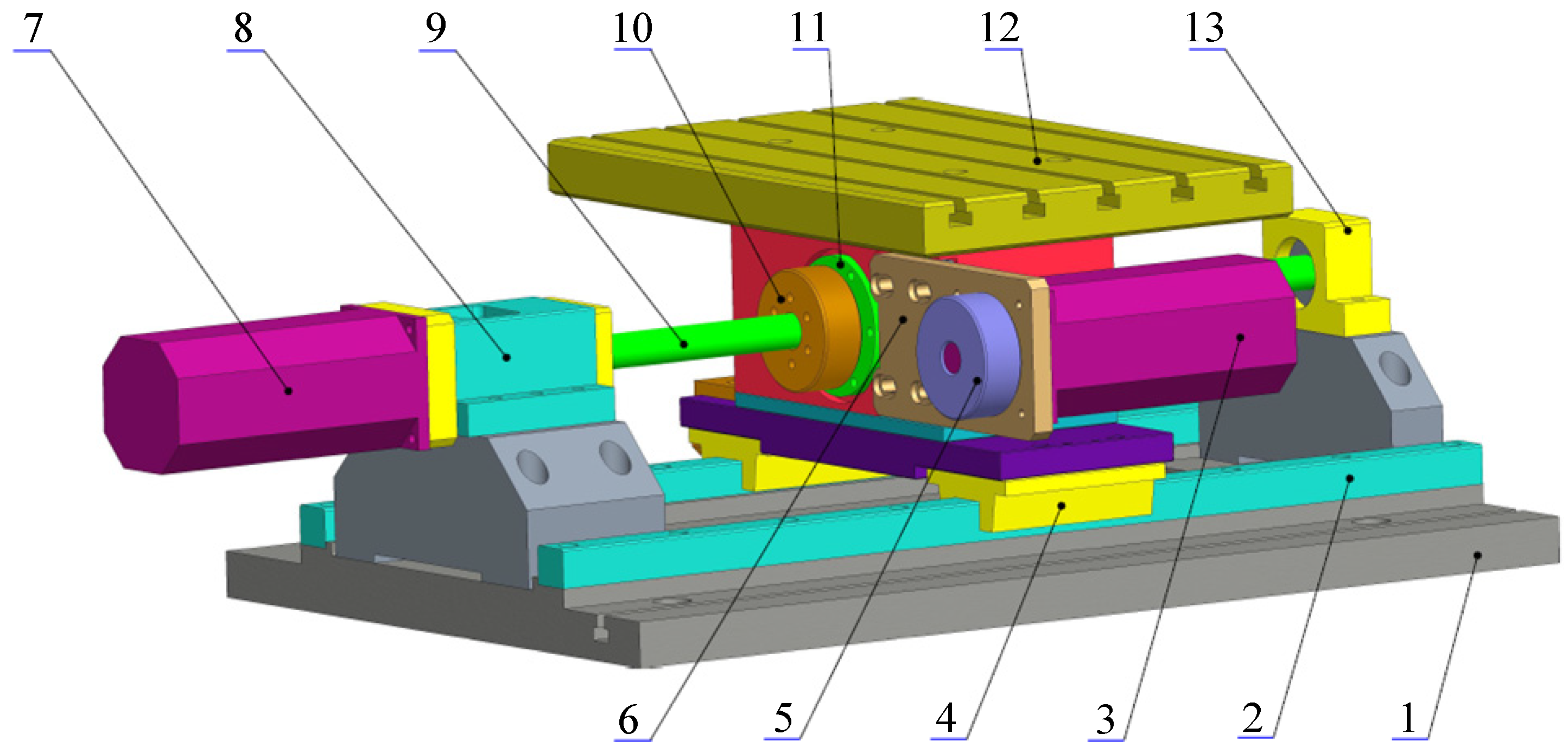
2.1. Nut Rotating Ball Screw Precision Transmission Mechanism

Figure 1 displays a sketch map for the micro-feed mechanism with a nut-rotating ball screw pair as a transmission component [32]. The meanings represented by the numbers are as follows: 1-Base, 2-Guide rail, 3-Nut servo motor, 4-Slide block, 5-Master synchronous belt wheel, 6-Nut motor mounting plate, 7-Screw servo motor, 8-Motor transmission seat, 9-Ball screw, 10-Slave synchronous belt wheel, 11-Rotating nut, 12-Table, and 13-Support bearing seat.

Power and displacement are transmitted to the table through a nut-rotating ball screw pair. The screw servo motor triggers the rotation of the ball screw via coupling, the nut servo motor drives the nut to rotate through a synchronous belt. The ball screw adopts a “fixed support” installation method, with a fixed end using a diagonal contact ball bearing and a supporting end using a radial ball bearing, and the table moves back and forth on the rolling guide rail.

The CNC motion controller allocates motion instructions for the screw servo motor and nut servo motor according to a certain algorithm based on the given motion requirements of the table. The table’s linear motion speed along the axial direction driven solely by the screw servo motor is indicated as V1, while that along the axial direction driven solely by the nut servo motor is represented by V2. Under the dual servo motor drive, the differential synthesis speed of the table approaches zero, that is Δ = V1 − V2 ≈ 0 avoids the crawling phenomenon caused by low-speed table motion under driving by an individual servo motor, allowing the differential table to achieve high-precision micro feed motion that a traditional servo system cannot achieve.

After repeated calculation of the system parameters, the critical crawling velocity of the table with a single screw drive system is obtained as approximately 2.5 mm/s. Several simulations were performed under the same parameters and the critical crawling velocity of the differential dual-drive system reached approximately 1.5 mm/s. By analyzing the output speed of the table under the constant velocity condition and the variable velocity condition of two types of drives, the conclusions are that the differential dual-drive system has better micro-feed performance at low speed and quicker responsiveness than the single-drive system [33].

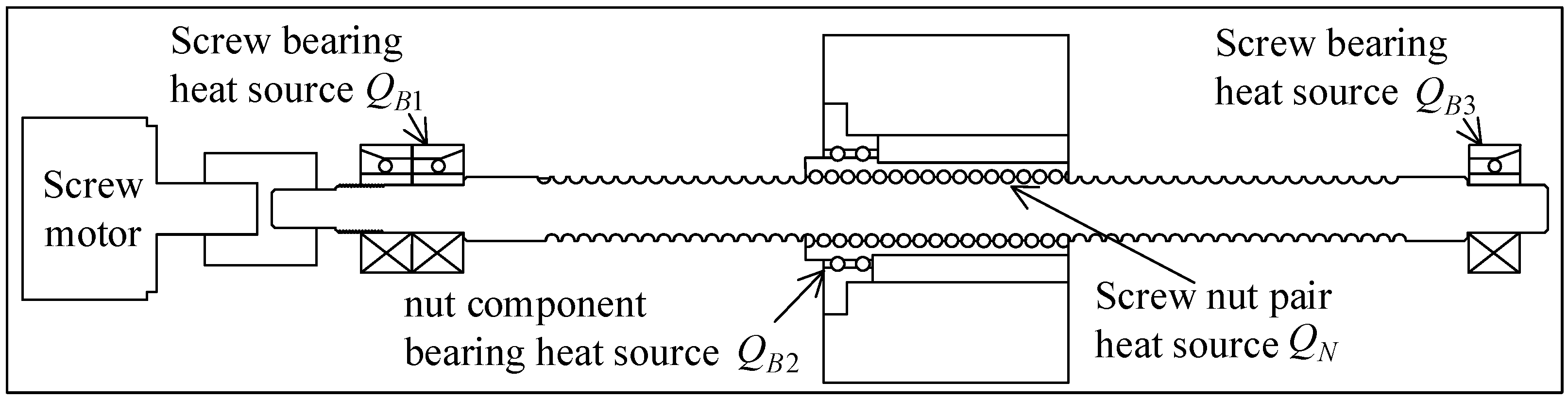
2.2. Heat Conduction Analysis of Nut-Rotating Ball Screw Pairs

Thermal conductivity analysis on the nut-rotating ball screw feed system ultimately focuses on the screw itself. Due to the fact that the machine tool’s feed accuracy is mostly affected by thermal deformation in the screw axis direction, assuming the uniform temperature distribution on the screw cross-section, with the screw being regarded as a one-dimensional thermal conductor with only temperature gradients in the axis direction. Therefore, the thermal conductivity equation of the one-dimensional rod is as follows.

$$\frac{{\partial }^{2}T(x,t)}{\partial x^2}=\frac{1}{{\alpha }_C}\frac{\partial T(x,t)}{\partial t}+\frac{4h}{\kappa d_0}\left[T(x,t)-T_f\right]$$

(1)

where $T(x,t)$ stands for temperature function on the screw, representing temperature change at time $t$ at position $x$ from the heat source; ${\alpha }_C$ is the thermal diffusivity, $\alpha =\kappa /\rho c$; $\kappa$ indicates thermal conductivity; $\rho$ represents screw density; $c$ indicates specific heat capacity; $h$ suggests a convective heat transfer coefficient between the external environment and the screw surface; $d_0$ stands for lead screw’s nominal diameter; $T_f$ indicates ambient temperature.

As shown in Figure 2, there are four major heat sources in the nut-rotating ball screw feed system: heat source $Q_{B1}$ near the motor end screw bearing, heat source $Q_{B2}$ at the nut component bearing, heat source $Q_N$ for the screw nut pair, and heat source $Q_{B3}$ far away from the motor end screw bearing. The screw motor is connected to the screw through a diaphragm coupling, and an insulation pad is installed inside the coupling. Therefore, the heat source at the screw motor has a negligible impact on the system temperature field. In addition, due to the fact that the nut motor transmits motion to the nut through a synchronous belt and has a large transmission distance, the heat source at the nut motor has no effect on the screw’s thermal deformation. According to the superposition principle, the heat source of the nut bearing and that of the screw nut pair can be superimposed to form $Q_{NB2}=Q_N+Q_{B2}$. During operation, the nut component shows forward and backward movements along the screw axis direction within the effective travel range of the screw. Therefore, $Q_{NB2}$ is regarded as a ring-shaped fixed heat source on the screw’s cylindrical surface.

In the case of combined action of multiple heat sources, as Equation (1) belongs to the second-order linear partial differential equation, based on the linear superposition principle, the screw’s temperature response at a given time and position can be determined by adding screw’s temperature responses under each single heat source, which is displayed below:

$$T_{total}(x,t)=\Sigma T_i(x,t)$$

(2)

in which $T_1(x,t)$ stands for temperature response resulting from heat source $Q_{B1}$; $T_2(x,t)$ represents temperature response resulting from heat source $Q_{NB2}$; $T_3(x,t)$ represents temperature response resulting from heat source $Q_{B3}$; $T_{total}(x,t)$ represents the sum of the screw’s temperature response under multiple heat sources.

2.3. Analysis of Temperature Field of the Nut-Rotating Ball Screw Pair under the Action of Heat Source

The screw temperature field at an equal distance from the heat source on both sides of the heat source exhibits symmetrical distribution, and the temperature response $T_2(x,t)$ caused by the heat source $Q_{NB2}$ is equal within the range of the nut stroke, that is, $\partial T_2(x,t)/\partial x=0$. The screw bearing can be detected at the screw terminal, therefore, the temperature response caused by the screw varies at different points. In this regard, it is of great necessity to investigate the temperature response on one side.

The screw temperature field is the solution to heat conduction Equation (1), but its analytical solution cannot be obtained. In the non-stationary stage of rapid heating or cooling of the screw, the screw’s internal thermal conductivity greatly increases relative to its convective heat transfer efficiency in the air. At this time, $\kappa >>h$. Therefore, in the non-stationary stage of screw temperature change, the convective heat transfer term in the thermal conduction equation is negligible. The screw transient thermal conduction equation is obtained as follows:

$$\frac{{\partial }^{2}T(x,t)}{\partial x^2}=\frac{1}{{\alpha }_C}\frac{\partial T(x,t)}{\partial t}$$

(3)

2.3.1. Constant Heat Source Temperature Response

Using one side of the screw as a constant power heat source and the boundary condition, the screw temperature field caused by the constant heat source is studied. Assuming that the initial temperature of the system is consistent with the environment, the initial condition is $T(x,0)=T_f$; If the temperature of a constant heat source is $T_m$, then the boundary condition is $T(0,t)=T_m$; The screw transient temperature field distribution is obtained by solving Equation (3):

$$T_t(x,t)={\Gamma }_{\max }\left[1-erf(\frac{x}{2\sqrt{{\alpha }_{C}t}})\right]+T_f$$

(4)

where $T_t(x,t)$ stands for the screw’s transient temperature value; ${\Gamma }_{\max }=T_m-T_f$ represents the screw’s temperature elevation after reaching thermal stability; $erf(x)$ is defined in mathematics as an error function:

$$erf(x)=\frac{2}{\sqrt{\pi }}{\displaystyle {\int }_0^x{e}^{-{\delta }^2}}d\delta$$

(5)

Equation (4) indicates that after a sufficiently long period of time, when the screw is insulated from the air, the steady-state temperature values at each point on the screw are equal to the heat source temperature $T_m$. However, this situation is not in line with actual working conditions, thus it is necessary to establish a steady-state temperature field model for the screw and to solve the screw’s steady-state temperature values at each point while taking into account convective heat transfer. When the screw temperature field reaches the steady state, the temperature will not change with time at each point, that is, $\partial T(x,t)/\partial t=0$. The screw steady-state heat conduction equation can be obtained from Equation (1):

$$\frac{{\partial }^{2}T(x,t)}{\partial x^2}=\frac{4h}{\kappa d_0}\left[T(x,t)-T_f\right]$$

(6)

The screw steady-state temperature field distribution acquired through solving Equation (6) is:

$$T_s(x,t)=C_1{e}^{-\sqrt{\frac{4h}{\kappa d_0}}x}+C_2{e}^{\sqrt{\frac{4h}{\kappa d_0}}x}+T_f$$

(7)

where $T_s(x,t)$ stands for the screw’s steady-state temperature value; $C_1$ and $C_2$ represent coefficients for the screw’s temperature rise, in degrees, and temperature distribution, respectively.

When taking convective heat transfer into account, the screw’s steady-state temperature rise value is ${\Gamma }_{\max }=T_s(x,t)-T_f$. The theoretical model of the screw temperature field under a constant heat source on one side can be obtained by combining Equations (4), (5) and (7):

$$T_c(x,t)=\left(C_1{e}^{-\sqrt{\frac{4h}{\kappa d_0}}x}+C_2{e}^{\sqrt{\frac{4h}{\kappa d_0}}x}\right)\left(1-\frac{2}{\sqrt{\pi }}{\displaystyle {\int }_0^{\frac{x}{2\sqrt{\alpha t}}}{e}^{-{\delta }^2}d\delta }\right)+T_f$$

(8)

The first of the two terms in Equation (8) represents the screw’s temperature rise distribution after steady state, while the second term represents the temperature changes at different points on the screw at different times.

2.3.2. Periodic Variation in Heat Source Temperature Response

When a periodic heat source is applied to the screw on one side, the screw’s temperature at each point is always in a non-steady state process of rising or falling, thus convective heat transfer between the air and screw can be ignored. Boundary conditions are:

$${\left.T(x,t)\right|}_{x=0}=T_0+T_1\sin (\omega t-\mathsf{\phi })$$

(9)

$T_0,T_1,\omega ,\mathsf{\phi }$ are all constants.

According to the boundary conditions in Equation (9), we solve Equation (3) to acquire the screw temperature response as follows:

$$T_p(x,t)=T_0+T_1{e}^{-x\sqrt{\frac{\omega }{2{\alpha }_C}}}\sin (\omega t-x\sqrt{\frac{\omega }{2{\alpha }_C}}-\mathsf{\phi })$$

(10)

From Equation (10), the screw temperature response at each point has the same frequency as the heat source, while the temperature amplitude at each point is:

$$A_m=T_0+T_1{e}^{-x\sqrt{\frac{\omega }{2{\alpha }_C}}}$$

(11)

From Equation (11), it can be seen that the temperature amplitude of the screw decreases exponentially with the increase in distance x, and the phase angles of each point are:

$$\mathsf{\phi }(x)=x\sqrt{\frac{\omega }{2{\alpha }_C}}+\mathsf{\phi }$$

(12)

From Equation (12), it can be seen that the phase angle at each point of the screw is different. As the distance x increases, the phase angle also increases, indicating that the temperature changes at each point of the screw relative to the heat source have a time lag.

2.3.3. Any Heat Source Temperature Response

The heat source of machine tools is variable under different working conditions, and there may be periodic or non-periodic changes in the heat source when processing multiple parts or processes. Due to the continuous variation in the heat source of the time domain, which satisfies Dirichlet boundary conditions, the heat source function can be expanded into a Fourier function with time t as the independent variable in the time domain. That is, the boundary conditions for any heat source are:

$$\begin{array}{l}{\left.T(x,t)\right|}_{x=0}=\frac{a_0}{2}+{\displaystyle \sum _{k=1}^{\infty }(a_k\cos kt+b_k\sin kt)}\\ =T_0+T_1\cos (\omega t-{\mathsf{\phi }}_1)+T_2\cos (\omega t-{\mathsf{\phi }}_2)+\cdots +T_n\cos (\omega t-{\mathsf{\phi }}_n)+\cdots \end{array}$$

(13)

Under any changing heat source, temperature values at various positions change in real time. At this time, the system’s internal heat conduction dominates, thus convective heat transfer between the air and the screw can be ignored. Boundary condition Equation (13) of any heat source is substituted into Equation (3) to obtain the screw temperature response function caused by any heat source:

$$T_a(x,t)=T_0+{\displaystyle \sum _{n=1}^{\infty }{T}_n{e}^{-x\sqrt{\frac{n\omega }{2{\alpha }_C}}}\cos (n\omega t-x\sqrt{\frac{n\omega }{2{\alpha }_C}}-{\mathsf{\phi }}_n)}$$

(14)

2.4. Thermal Resistance Network Analysis of Nut-Rotating Ball Screw Transmission Mechanism

Using the thermal resistance network method to explore the steady-state temperature field distribution of the system exhibits the advantages of short simulation time, high computational efficiency, and strong real-time performance. The research object is subdivided using temperature nodes, and there is conduction or convective heat transfer resistance between each temperature node, forming a thermal resistance network. Based on the principle of thermoelectric analogy, Kirchhoff’s law is followed to establish a thermal balance equation for each temperature node.

2.4.1. Heat Transfer Analysis

In this study, the transmission component used in the dual-drive mechanism is the DIR-type nut-rotating ball screw pair, which is a device integrating the single nut ball screw with the supporting bearing. In other words, the outer ring of the supporting bearing in the nut assembly can be integrated with the flange in the nut assembly. In addition, the inner ring of the supporting bearing is integrated with the outer ring of the rotating nut. The heat source distribution of this mechanism shows the difference with that of conventional mechanisms with the nut and the screw being driven, respectively. According to thermodynamic research and achievements on bearings and conventional screw drive mechanisms, both domestically and internationally, thermal analysis is performed on the dual-drive mechanism.

The dual-drive nut-rotating ball screw pair is an open heat transfer system. During the operation, there is a large amount of heat generated due to power loss and heat dissipation. According to the law of energy conservation, the entire dual-drive ball screw system ultimately reaches a thermal equilibrium state. In mechanical transmission systems, heat transfer mainly occurs in the form of thermal conduction and convection, and thermal radiation can be ignored. Additionally, part of the heat generated by power loss is transferred to other components in contact through thermal conduction, while another part is transferred to the internal air or external environment of the system through thermal convection.

Taking the dual-drive nut-rotating ball screw pair as the research object, the heat transfer of the ball screw pair system under the action of the screw nut heat source and the nut component bearing heat source is first analyzed, as displayed in Figure 3. Similarly, the effects of other heat sources are explored.

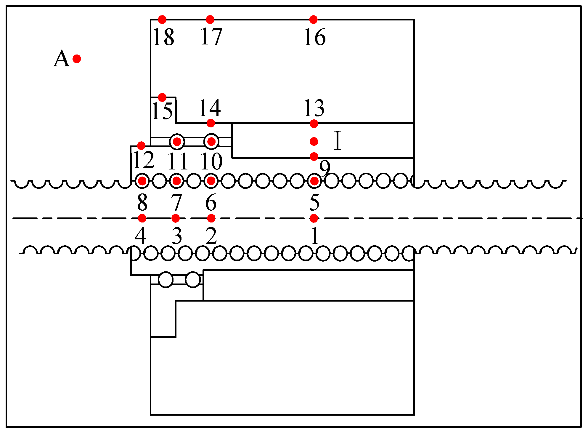
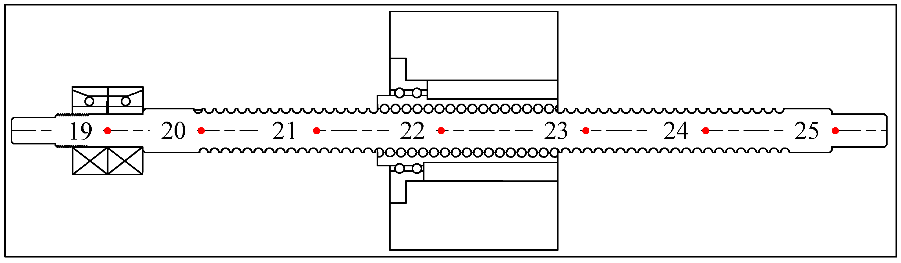
2.4.2. Hot Node Layout

According to the thermal resistance network approach, we should arrange thermal nodes as densely as possible in important parts of the system and components that require specific temperature values. Through the heat transfer analysis of the dual-drive nut-rotating ball screw pair, it is found that the heat generated due to power loss significantly affects the entire ball screw pair’s temperature field. Therefore, temperature nodes need to be arranged at the heat source point. In addition, temperature nodes should also be arranged at the parts in the ball screw pair that have thermal convection with the internal air or external environment.

From Figure 4, the temperature node arrangement of the dual-drive ball screw pair is shown under the screw nut heat source and the nut-component-bearing heat source. Figure 5 and Figure 6, respectively, show the temperature node arrangement of the screw when the left-bearing heat source is applied and the temperature node arrangement of the screw when the right-bearing heat source is applied.

The red “•” in Figure 4, Figure 5 and Figure 6 represent the temperature node positions arranged in the system.

Table 1. Meaning of temperature nodes for dual-drive nut-rotating ball screw pairs.

Node	Location of Each Temperature Node	Node Temperature
1	The temperature of the screw section at a distance of 25 mm from the right end of the rotating nut	$T_1$
2	The temperature of the screw section at the right support ball section in the nut assembly	$T_2$
3	The temperature of the screw section at the left support ball section in the nut assembly	$T_3$
4	The temperature of the screw section at a distance of 4 mm from the left end of the rotating nut	$T_4$
5	Surface temperature of the nut inner ring at a distance of 25 mm from the right end of the rotating nut	$T_5$
6	The surface temperature of the nut inner ring at the right support ball section in the nut assembly	$T_6$
7	The surface temperature of the nut inner ring at the left support ball section in the nut assembly	$T_7$
8	Surface temperature of the nut inner ring at a distance of 4 mm from the left end of the rotating nut	$T_8$
9	Surface temperature of the nut outer ring at a distance of 25 mm from the right end of the rotating nut	$T_9$
10	The average temperature of the right support ball in the nut assembly	$T_{10}$
11	The average temperature of the left support ball in the nut assembly	$T_{11}$
12	Surface temperature of the nut outer ring at a distance of 4 mm from the left end of the rotating nut	$T_{12}$
13	Surface temperature of the nut seat inner ring at a distance of 25 mm from the right end of the rotating nut	$T_{13}$
14	The surface temperature of the nut seat inner ring at the right support ball section in the nut assembly	$T_{14}$
15	Surface temperature of the nut seat inner ring at the flange section in the nut assembly	$T_{15}$
16	Surface temperature of the nut seat outer ring at a distance of 25 mm from the right end of the rotating nut	$T_{16}$
17	The surface temperature of the nut seat outer ring at the right support ball section in the nut assembly	$T_{17}$
18	Surface temperature of the nut seat outer ring at the flange section in the nut assembly	$T_{18}$
I	Air temperature between nut seat and rotating nut	$T_I$
19, 32	The temperature of the screw section at the left bearing section of the screw	$T_{19}$$, T_{32}$
20, 31	The temperature of the screw section at a distance of 40 mm from the bearing section on the left side of the screw	$T_{20}$$, T_{31}$
21, 30	The temperature of the screw section at a distance of 100 mm from the bearing section on the left side of the screw	$T_{21}$$, T_{30}$
22, 29	The temperature of the screw section at a distance of 160 mm from the bearing section on the left side of the screw	$T_{22}$$, T_{29}$
23, 28	The temperature of the screw section at a distance of 220 mm from the bearing section on the left side of the screw	$T_{23}$$, T_{28}$
24, 27	The temperature of the screw section at a distance of 280 mm from the bearing section on the left side of the screw	$T_{24}$$, T_{27}$
25, 26	The temperature of the screw section at the bearing section on the right side of the screw	$T_{25}$$, T_{26}$
A	External environmental temperature	$T_A$

lists the serial numbers and temperature symbols for each node.

2.4.3. Establishment of a Thermal Resistance Network

Temperature difference is the driving force for heat transfer, and thermal resistance is its resistance. The ratio of the two is the heat transfer amount (heat flux). According to heat transfer analysis of the dual-drive nut-rotating ball screw pair and arrangement of heat nodes, the thermal resistance network model is constructed for the dual-drive mechanism, as shown in Figure 7, Figure 8 and Figure 9.

In Figure 7, Figure 8 and Figure 9, the symbol “$\otimes$” represents the system’s heat source point. R represents thermal resistance between two temperature nodes, where the subscript “C” represents heat transfer between the two components through thermal conduction, and the subscript “V” represents heat convection between the components and the internal air or external environment of the system. The arrow represents the heat flow direction of two temperature nodes.

2.4.4. Heat Balance Equation

Analogous to Kirchhoff’s law, the temperature difference between two temperature nodes is equivalent to the voltage in the circuit, and the thermal resistance between temperature nodes is equivalent to the resistance in the circuit. Therefore, the ratio of temperature difference to thermal resistance is equivalent to the current in the circuit. When the system reaches thermal equilibrium, the heat flow entering and exiting the temperature node is equal.

For the convenience of analyzing the system’s temperature field, before listing the system thermal balance equation, the following assumptions and simplifications are made for the dual-drive nut-rotating ball screw system:

(1)

The dual drive nut rotating ball screw pair has reached a thermal equilibrium state;

(2)

Due to the temperature difference between various components in the mechanical transmission process being less than 200 °C, the influence of thermal radiation is ignored;

(3)

The material of the components in the nut-rotating ball screw pair is isotropic, thus the heat flow direction does not affect the magnitude of thermal resistance;

(4)

The thermal conductivity of each component in the system remains constant during temperature changes;

(5)

Contact thermal resistance across various components in the nut-rotating ball screw pair is neglected;

(6)

The external environment in which the system is located is at a constant temperature of 25 °C;

In line with Kirchhoff’s law and the above assumptions, the thermal balance equations of every temperature node in the double drive nut rotating ball screw transmission system are listed as follows:

$$\left(\frac{1}{R_{1VA}}+\frac{1}{R_{1C2}}+\frac{1}{R_{1C5}}\right)T_1-\frac{1}{R_{1C2}}{T}_2-\frac{1}{R_{1C5}}{T}_5-\frac{1}{R_{1VA}}{T}_A=0$$

(15)

$$\frac{1}{R_{1C2}}{T}_1-\left(\frac{1}{R_{1C2}}+\frac{1}{R_{2C3}}+\frac{1}{R_{2C6}}+\frac{1}{R_{2VA}}\right)T_2+\frac{1}{R_{2C3}}{T}_3+\frac{1}{R_{2C6}}{T}_6+\frac{1}{R_{2VA}}{T}_A=0$$

(16)

$$\frac{1}{R_{2C3}}{T}_2-\left(\frac{1}{R_{2C3}}+\frac{1}{R_{3C7}}+\frac{1}{R_{3C4}}+\frac{1}{R_{3VA}}\right)T_3+\frac{1}{R_{3C4}}{T}_4+\frac{1}{R_{3C7}}{T}_7+\frac{1}{R_{3VA}}{T}_A=0$$

(17)

$$\frac{1}{R_{3C4}}{T}_3-\left(\frac{1}{R_{3C4}}+\frac{1}{R_{4C8}}+\frac{1}{R_{4VA}}\right)T_4+\frac{1}{R_{4C8}}{T}_8+\frac{1}{R_{4VA}}{T}_A=0$$

(18)

$$\frac{1}{R_{1C5}}{T}_1-\left(\frac{1}{R_{5C6}}+\frac{1}{R_{1C5}}+\frac{1}{R_{5C9}}\right)T_5+\frac{1}{R_{5C6}}{T}_6+\frac{1}{R_{5C9}}{T}_9=-Q_5$$

(19)

$$\frac{1}{R_{2C6}}{T}_2+\frac{1}{R_{5C6}}{T}_5-\left(\frac{1}{R_{2C6}}+\frac{1}{R_{5C6}}+\frac{1}{R_{6C7}}+\frac{1}{R_{6C10}}\right)T_6+\frac{1}{R_{6C7}}{T}_7+\frac{1}{R_{6C10}}{T}_{10}=-Q_6$$

(20)

$$\frac{1}{R_{3C7}}{T}_3+\frac{1}{R_{6C7}}{T}_6-\left(\frac{1}{R_{6C7}}+\frac{1}{R_{3C7}}+\frac{1}{R_{7C8}}+\frac{1}{R_{7C11}}\right)T_7+\frac{1}{R_{7C8}}{T}_8+\frac{1}{R_{7C11}}{T}_{11}=-Q_7$$

(21)

$$\frac{1}{R_{4C8}}{T}_4+\frac{1}{R_{7C8}}{T}_7-\left(\frac{1}{R_{7C8}}+\frac{1}{R_{4C8}}+\frac{1}{R_{8C12}}\right)T_8+\frac{1}{R_{8C12}}{T}_{12}=-Q_8$$

(22)

$$\frac{1}{R_{5C9}}{T}_5-\left(\frac{1}{R_{5C9}}+\frac{1}{R_{9C10}}+\frac{1}{R_{9VI}}\right)T_9+\frac{1}{R_{9C10}}{T}_{10}+\frac{1}{R_{9VI}}{T}_I=0$$

(23)

$$\frac{1}{R_{6C10}}{T}_6+\frac{1}{R_{9C10}}{T}_9-\left(\frac{1}{R_{6C10}}+\frac{1}{R_{9C10}}+\frac{1}{R_{10C11}}+\frac{1}{R_{10C14}}\right)T_{10}+\frac{1}{R_{10C11}}{T}_{11}+\frac{1}{R_{10C14}}{T}_{14}=-Q_{10}$$

(24)

$$\frac{1}{R_{7C11}}{T}_7+\frac{1}{R_{10C11}}{T}_{10}-\left(\frac{1}{R_{7C11}}+\frac{1}{R_{10C11}}+\frac{1}{R_{11C12}}+\frac{1}{R_{11C15}}\right)T_{11}+\frac{1}{R_{11C12}}{T}_{12}+\frac{1}{R_{11C15}}{T}_{15}=-Q_{11}$$

(25)

$$\frac{1}{R_{8C12}}{T}_8+\frac{1}{R_{11C12}}{T}_{11}-\left(\frac{1}{R_{8C12}}+\frac{1}{R_{11C12}}+\frac{1}{R_{12VA}}\right)T_{12}+\frac{1}{R_{12VA}}{T}_A=0$$

(26)

$$\left(\frac{1}{R_{13C16}}+\frac{1}{R_{13C14}}+\frac{1}{R_{13VI}}\right)T_{13}-\frac{1}{R_{13C14}}{T}_{14}-\frac{1}{R_{13C16}}{T}_{16}-\frac{1}{R_{13VI}}{T}_I=0$$

(27)

$$\frac{1}{R_{10C14}}{T}_{10}+\frac{1}{R_{13C14}}{T}_{13}-\left(\frac{1}{R_{10C14}}+\frac{1}{R_{13C14}}+\frac{1}{R_{14C15}}+\frac{1}{R_{14C17}}\right)T_{14}+\frac{1}{R_{14C15}}{T}_{15}+\frac{1}{R_{14C17}}{T}_{17}=0$$

(28)

$$\frac{1}{R_{11C15}}{T}_{11}+\frac{1}{R_{14C15}}{T}_{14}-\left(\frac{1}{R_{11C15}}+\frac{1}{R_{14C15}}+\frac{1}{R_{15C18}}\right)T_{15}+\frac{1}{R_{15C18}}{T}_{18}=0$$

(29)

$$\frac{1}{R_{13C16}}{T}_{13}-\left(\frac{1}{R_{13C16}}+\frac{1}{R_{16C17}}+\frac{1}{R_{16VA}}\right)T_{16}+\frac{1}{R_{16C17}}{T}_{17}+\frac{1}{R_{16VA}}{T}_A=0$$

(30)

$$\frac{1}{R_{14C17}}{T}_{14}+\frac{1}{R_{16C17}}{T}_{16}-\left(\frac{1}{R_{14C17}}+\frac{1}{R_{16C17}}+\frac{1}{R_{17C18}}+\frac{1}{R_{17VA}}\right)T_{17}+\frac{1}{R_{17C18}}{T}_{18}+\frac{1}{R_{17VA}}{T}_A=0$$

(31)

$$\frac{1}{R_{15C18}}{T}_{15}+\frac{1}{R_{17C18}}{T}_{17}-\left(\frac{1}{R_{15C18}}+\frac{1}{R_{17C18}}+\frac{1}{R_{18VA}}\right)T_{18}+\frac{1}{R_{18VA}}{T}_A=0$$

(32)

$$\frac{1}{R_{9VI}}{T}_9+\frac{1}{R_{13VI}}{T}_{13}-\left(\frac{1}{R_{9VI}}+\frac{1}{R_{13VI}}+\frac{1}{R_{IVA}}\right)T_I+\frac{1}{R_{IVA}}{T}_A=0$$

(33)

$$\left(\frac{1}{R_{19C20}}+\frac{1}{R_{19VA}}\right)T_{19}-\frac{1}{R_{19C20}}{T}_{20}-\frac{1}{R_{19VA}}{T}_A=Q_{19}$$

(34)

$$\frac{1}{R_{19C20}}{T}_{19}-\left(\frac{1}{R_{19C20}}+\frac{1}{R_{20C21}}+\frac{1}{R_{20VA}}\right)T_{20}+\frac{1}{R_{20C21}}{T}_{21}+\frac{1}{R_{20VA}}{T}_A=0$$

(35)

$$\frac{1}{R_{20C21}}{T}_{20}-\left(\frac{1}{R_{20C21}}+\frac{1}{R_{21C22}}+\frac{1}{R_{21VA}}\right)T_{21}+\frac{1}{R_{21C22}}{T}_{22}+\frac{1}{R_{21VA}}{T}_A=0$$

(36)

$$\frac{1}{R_{21C22}}{T}_{21}-\left(\frac{1}{R_{21C22}}+\frac{1}{R_{22C23}}+\frac{1}{R_{22VA}}\right)T_{22}+\frac{1}{R_{22C23}}{T}_{23}+\frac{1}{R_{22VA}}{T}_A=0$$

(37)

$$\frac{1}{R_{22C23}}{T}_{22}-\left(\frac{1}{R_{22C23}}+\frac{1}{R_{23C24}}+\frac{1}{R_{23VA}}\right)T_{23}+\frac{1}{R_{23C24}}{T}_{24}+\frac{1}{R_{23VA}}{T}_A=0$$

(38)

$$\frac{1}{R_{23C24}}{T}_{23}-\left(\frac{1}{R_{23C24}}+\frac{1}{R_{24C25}}+\frac{1}{R_{24VA}}\right)T_{24}+\frac{1}{R_{24C25}}{T}_{25}+\frac{1}{R_{24VA}}{T}_A=0$$

(39)

$$\frac{1}{R_{24C25}}{T}_{24}-\left(\frac{1}{R_{24C25}}+\frac{1}{R_{25VA}}\right)T_{25}+\frac{1}{R_{25VA}}{T}_A=0$$

(40)

$$\left(\frac{1}{R_{26C27}}+\frac{1}{R_{26VA}}\right)T_{26}-\frac{1}{R_{26C27}}{T}_{27}-\frac{1}{R_{26VA}}{T}_A=Q_{26}$$

(41)

$$\frac{1}{R_{26C27}}{T}_{26}-\left(\frac{1}{R_{26C27}}+\frac{1}{R_{27C28}}+\frac{1}{R_{27VA}}\right)T_{27}+\frac{1}{R_{27C28}}{T}_{28}+\frac{1}{R_{27VA}}{T}_A=0$$

(42)

$$\frac{1}{R_{27C28}}{T}_{27}-\left(\frac{1}{R_{27C28}}+\frac{1}{R_{28C29}}+\frac{1}{R_{28VA}}\right)T_{28}+\frac{1}{R_{28C29}}{T}_{29}+\frac{1}{R_{28VA}}{T}_A=0$$

(43)

$$\frac{1}{R_{28C29}}{T}_{28}-\left(\frac{1}{R_{28C29}}+\frac{1}{R_{29C30}}+\frac{1}{R_{29VA}}\right)T_{29}+\frac{1}{R_{29C30}}{T}_{30}+\frac{1}{R_{29VA}}{T}_A=0$$

(44)

$$\frac{1}{R_{29C30}}{T}_{29}-\left(\frac{1}{R_{29C30}}+\frac{1}{R_{30C31}}+\frac{1}{R_{30VA}}\right)T_{30}+\frac{1}{R_{30C31}}{T}_{31}+\frac{1}{R_{30VA}}{T}_A=0$$

(45)

$$\frac{1}{R_{30C31}}{T}_{30}-\left(\frac{1}{R_{30C31}}+\frac{1}{R_{31C32}}+\frac{1}{R_{31VA}}\right)T_{31}+\frac{1}{R_{31C32}}{T}_{32}+\frac{1}{R_{31VA}}{T}_A=0$$

(46)

$$\frac{1}{R_{31C32}}{T}_{31}-\left(\frac{1}{R_{31C32}}+\frac{1}{R_{32VA}}\right)T_{32}+\frac{1}{R_{32VA}}{T}_A=0$$

(47)

$$T_A=25 °\mathrm{C}$$

(48)

The thermal balance equation of the nut-rotating ball screw transmission system in matrix form is written as follows:

$$A_{m\times n}{T}_{n\times 1}=B_{m\times 1}$$

(49)

where $A_{m\times n}$ is the temperature coefficient matrix composed of the reciprocal of thermal resistance; $T_{n\times 1}$ stands for the node temperature matrix; $B_{m\times 1}$ indicates a matrix composed of heat source points, with non-heat source point values considered as zero.

2.5. Thermal Error Analysis of Nut-Rotating Ball Screw

Thermal deformation error is an important component of motion error in micro feed systems, and for precision feed control systems, it is necessary to consider research. The nut-rotating ball screw in the micro feed mechanism in this article utilizes the fixed support in one terminal, whereas the free extension is used in the other terminal for installation. Thermal elongation at the ball screw terminal represents the sum of the ball screw thermal error. Ignoring the thread of the ball screw and treating it as a smooth cylinder, the ball screw’s thermal error principle can be observed in Figure 10.

Divide the screw into individual “micro units” $\Delta L_0$. For the accurate prediction of thermal error, assume $\Delta L_0\to 0$, and following a period of time when the heat source acts on it, the temperature changes to $T\left(x,t\right)-T_0$. Thermal error of the screw’s “micro units” can be expressed as:

$$\Delta L(x)-\Delta L_0={\alpha }_T\left[T\left(x,t\right)-T_0\right]\Delta L_0$$

(50)

where $\Delta L(x)-\Delta L_0$ stands for the “micro unit”’s thermal elongation and ${\alpha }_T$ indicates the screw’s average linear expansion coefficient.

Thermal error at the screw terminal is acquired by adding all micro unit’s thermal elongations, that is, the screw’s total thermal error can be expressed as:

$$E={\displaystyle {\int }_0^L{\alpha }_T[T\left(x,t\right)-T_0]d\delta }={\displaystyle \sum _{i=1}^n{\alpha }_T[T_i(x,t)-T_0]\Delta L_0}$$

(51)

3. Numerical Analysis and Simulation Calculation

Table 2. Thermodynamic parameters of the nut-rotating ball screw precision transmission mechanism.

Parameters	Values	Unit
Ball screw diameter $d_0$	16	$\mathrm{mm}$
Axial force $F_a$	500	$\mathrm{N}$
Thermal conductivity $\kappa$	50	$\mathrm{W}/(\mathrm{m}\cdot \mathrm{K})$
Thermal diffusivity ${\alpha }_C$	$1.04\times {10}^{-5}$	${\mathrm{m}}^2/\mathrm{s}$
Lubricant kinematic viscosity $v_0$	40	$\mathrm{cst}$ or ${\mathrm{mm}}^2/\mathrm{s}$
Average linear expansion coefficient of screw ${\alpha }_T$	$11.8\times {10}^{-6}$	$\mathrm{mm}/ °\mathrm{C}$

presents the thermodynamic parameters of the micro feed system for the dual-drive nut-rotating ball screw pair. The screw’s fixed end adopts an angular contact ball bearing model of 7210AC, and the free support end adopts a radial ball bearing model of 6201. Based on the design parameters and empirical parameters of the nut-rotating ball screw precision transmission mechanism shown in Figure 1, an analysis program is written using Matlab R2016b numerical calculation software.

3.1. Thermodynamic Model Parameter Calculation of the Nut-Rotating Ball Screw Transmission Mechanism

As long as the thermal resistance value between nodes and heat generation at the heat source point are obtained, coefficients of matrices $A_{m\times n}$ and $B_{m\times 1}$ in Equation (49) can be determined. Then, numerical calculations can be carried out using Matlab to solve the specific temperature values of each node of the screw when the system is under single/dual driving conditions, respectively.

3.1.1. Heat Generation Calculation

According to a previous analysis, two heat source types are available for the nut-rotating ball screw transmission mechanism: (1) calculation of heat production from the screw support bearing and the bearing in the nut assembly; (2) Calculation of heat production at the screw–nut contact point.

• Heat generation calculation for rolling bearings

Rolling bearings mainly generate heat through friction. The friction moment method is used to calculate heat produced through bearing under a given speed and friction moment. Its calculation formula is:

$$Q_B=1.047\times {10}^{-4}{n}_B{M}_B$$

(52)

where $Q_B$ indicates heat produced through bearing $(\mathrm{W})$; $n_B$ represents bearing speed $(\mathrm{RPM})$; $M_B$ stands for frictional torque acting on the bearing $(\mathrm{N}\cdot \mathrm{mm})$.

Friction torque acting on rolling bearings is calculated based on the Palmgren empirical formula:

$$M_B=M_1+M_2$$

(53)

$$M_1=f_{1}P{d}_m$$

(54)

$$f_1=\left\{\begin{array}{ll}0.0013\times {(P_0/C_0)}^{0.33}\hfill & \mathrm{Single}\text{-}\mathrm{row} \mathrm{installation}\hfill \\ 0.001\times {(P_0/C_0)}^{0.33}\hfill & \mathrm{Double}\text{-}\mathrm{row} \mathrm{installation}\hfill \end{array}\right.$$

(55)

$$P=\left\{\begin{array}{ll}{P}_a+0.1P_r\hfill & \mathrm{Single}\text{-}\mathrm{row} \mathrm{installation}\hfill \\ 1.44P_a-0.1P_r\hfill & \mathrm{Double}\text{-}\mathrm{row} \mathrm{installation}\hfill \end{array}\right.$$

(56)

$$M_2=\left\{\begin{array}{ll}{10}^{-7}{f}_0{(v_0{n}_B)}^{2/3}{d}_m^3\hfill & v_0{n}_B\ge 2000\hfill \\ 160\times {10}^{-7}{f}_0{d}_m^3\hfill & v_0{n}_B<2000\hfill \end{array}\right.$$

(57)

where $M_1$ is the friction torque during startup and low-speed operation $(\mathrm{N}\cdot \mathrm{mm})$; $M_2$ represents friction torque associated with the bearing model, lubricating grease, and speed $(\mathrm{N}\cdot \mathrm{mm})$; $f_1$ is a coefficient associated with the load and bearing type; $P$ represents the external load of bearing $(\mathrm{N})$; $d_m$ accounts for the pitch diameter of bearing $(\mathrm{mm})$; $P_0$ suggests equivalent static load of bearing $(\mathrm{N})$; $C_0$ stands for the basic rated static load of bearing $(\mathrm{N})$; $P_a$ indicates axial load on bearing $(\mathrm{N})$; $P_r$ presents radial load on bearing $(\mathrm{N})$; $v_0$ is lubricant viscosity ($\mathrm{cst}$ or ${\mathrm{mm}}^2/\mathrm{s}$); $f_0$ is an empirical coefficient associated with bearing model and lubricant, with $f_0=4$ for double-row installation and $f_0=2$ for single-row installation.

2.

Calculation of heat generation at the contact point of the screw and the nut

The frictional heat produced through the nut-rotating ball screw pair can be determined by adding the heat generated by the rotating nut and that generated by the screw:

$$Q_{NS}=1.047\times {10}^{-4}\left(n_N{M}_N+n_S{M}_S\right)$$

(58)

where $Q_{NS}$ is heat produced at the nut screw pair contact point $(\mathrm{W})$; $n_N$ stands for the nut rotational speed (RPM); $n_S$ indicates the screw rotational speed (RPM); $M_N$ indicates the mut friction torques $(\mathrm{N}\cdot \mathrm{mm})$, which can be obtained from kinematic analysis; $M_S$ stands for the screw friction torque $(\mathrm{N}\cdot \mathrm{mm})$, which can also be obtained from kinematic analysis.

3.1.2. Thermal Resistance Calculation

The size of thermal resistance represents the ability to hinder heat transfer. According to heat transfer theory, in a one-dimensional steady-state heat transfer process, thermal resistance is divided into conduction resistance and convective heat transfer resistance.

3.

Calculation of conduction thermal resistance of thin-walled cylinders

$$R_C=\frac{\ln \left(d/D\right)}{2\pi l\kappa }$$

(59)

where $d$ is the outer diameter of the thin cylinder $(\mathrm{m})$; $D$ is the inner diameter of a thin cylinder $(\mathrm{m})$; $\kappa$ is the thermal conductivity of the material $\left[\mathrm{W}/\left(\mathrm{m}\cdot \mathrm{K}\right)\right]$; $l$ is the axial length of a thin cylinder $(\mathrm{m})$.

4.

Calculation of Conduction Thermal Resistance of Solid Bodies

$${R^{\prime }}_C=\frac{l^{\prime }}{A\kappa }$$

(60)

where $l^{\prime }$ stands for heat transfer length of solid body $(\mathrm{m})$; $A$ is thermal conductivity area vertical to the heat flow direction $({\mathrm{m}}^2)$.

5.

Calculation of convective heat transfer resistance

$$R_V=\frac{1}{\alpha S}$$

(61)

where $\alpha$ stands for convective heat transfer coefficient $[{\mathrm{W}/(\mathrm{m}}^2\cdot \mathrm{K})]$ and $S$ indicates the area of convective heat transfer $({\mathrm{m}}^2)$.

3.1.3. Calculation of Convective Heat Transfer Coefficient

Based on the model for calculating thermal resistance, when the size of each component is determined, its thermal resistance value will be determined by the thermal conductivity and convective heat transfer coefficient. Within a certain temperature range, the thermal conductivity coefficient can be considered a constant value, which is only related to the properties of the material. Therefore, the calculation of the convective heat transfer coefficient will be a key factor for calculating thermal resistance value and temperature distribution.

6.

Calculating the convective heat transfer coefficient of rotating components with the external environment

$$\mathrm{Re}=\frac{\omega \times d^2}{v_f}$$

(62)

$$Nu=0.133{\mathrm{Re}}^{2/3}{\mathrm{Pr}}^{1/3}\left(\mathrm{Re}<4.3\times {10}^5,0.7<\mathrm{Pr}<670\right)$$

(63)

$$\alpha =\frac{Nu\cdot \lambda }{d}$$

(64)

where $\mathrm{Re}$ indicates the Reynolds number; $\omega$ represents the component’s rotational angular velocity $(\mathrm{rad}/\mathrm{s})$; $d$ is the diameter of the convective heat transfer part in the rotating component $(\mathrm{m})$; $v_f$ is the air kinematic viscosity at $25 °\mathrm{C}$; $v_f=15.5\times {10}^{-6}{\mathrm{m}}^2/\mathrm{s}$; $Nu$ is the Nusselt number; $\mathrm{Pr}$ stands for Prandtl number, while $\mathrm{Pr}$ of air is $\mathrm{Pr}=0.72$; $\alpha$ suggests convective heat transfer coefficient of the rotating component with external air $[{\mathrm{W}/(\mathrm{m}}^2\cdot \mathrm{K})]$; $\lambda$ indicates thermal conductivity of the external air, at $25 °\mathrm{C}$, take $\lambda =2.54\times {10}^{-2}\mathrm{W}/(\mathrm{m}\cdot \mathrm{K})$.

7.

Calculating natural convection heat transfer coefficient

The convective heat transfer coefficient between components in a stationary state and the external environment is calculated as follows:

$$Gr=\frac{g\beta l^3\Delta t}{v_f^2}$$

(65)

$$Nu=C{(Gr\cdot \mathrm{Pr})}^n$$

(66)

$$\alpha =\frac{Nu\cdot \lambda }{l}$$

(67)

where $G_r$ is the Grayshev quasi number; $g$ is the gravitational acceleration, taken as $g=9.8 {\mathrm{m}/\mathrm{s}}^2$; $\beta$ is the coefficient of expansion of the external air, taken as $\beta =1/273$; $l$ is the length of heat flux $(\mathrm{m})$; $\Delta t$ is the temperature difference between the stationary component and the external environment, taken as $\Delta t=10 °\mathrm{C}$; $C$, $n$ are both constants, depending on the liquid state and heat source of the fluid.

The specific values are shown in

Table 3. The values of $C$ and $n$.

$\mathit{C}$	$\mathit{n}$	Scope of Application	Location of Heat Exchange Surface	Flow Pattern
0.59	1/4	${10}^4\le (Gr\cdot \mathrm{Pr})\le {10}^9$	Vertical flat wall	laminar flow
0.12	1/3	${10}^9\le (Gr\cdot \mathrm{Pr})\le {10}^{12}$	Vertical flat wall	turbulence
0.54	1/4	${10}^5\le (Gr\cdot \mathrm{Pr})\le 2\times {10}^7$	Horizontal wall facing downwards	laminar flow
0.14	1/3	$2\times {10}^7\le (Gr\cdot \mathrm{Pr})\le 3\times {10}^{10}$	Horizontal wall facing upwards	turbulence
0.27	1/4	$3\times {10}^5\le (Gr\cdot \mathrm{Pr})\le 3\times {10}^{10}$	Horizontal wall facing downwards	laminar flow

. The convective heat transfer coefficient in actual calculation is generally taken as 3–10 times the theoretical calculation result, while in this article, the convective heat transfer coefficient is taken as 10 times the theoretical calculation value.

3.2. Node Temperature of Nut-Rotating Ball Screw under a Single Heat Source Condition for Bearing

Figure 11, Figure 12, Figure 13, Figure 14, Figure 15 and Figure 16 present the temperature values of each node in the left bearing of the screw under the action of a single heat source. Obviously, with increasing distance from the heat source point, the steady-state temperature value of the node rapidly decays. At a specific point away from the heat source at this intensity, with the screw speed reaching a certain value, the temperature of that node will maintain a thermal equilibrium state. This indicates that when the screw speed reaches a certain value, the incoming heat and outgoing heat will always be consistent at that point. At nodes far from the heat source, with increasing screw speed, the temperature exhibits first a slight increase and then a decrease and tends toward room temperature because of an increase in convective heat transfer intensity between the screw speed and the air. As the temperature changes caused by heat sources are mainly concentrated near the heat source point, when considering temperature field changes, it becomes necessary to mainly investigate the temperature changes near the heat source point. The temperature field changes far away from the heat source point are relatively small. The variation pattern of the temperature field of the screw under the action of a single heat source on the right bearing of the screw is similar.

3.3. Node Temperature of Screw under a Single Heat Source Condition for Nut–Screw Pair

Figure 17, Figure 18, Figure 19 and Figure 20 show the temperature values of node 4, node 8, node 10, and node 11 of the screw under the single heat source condition for the nut–screw pair as a function of the nut rotation speed and composite rotation speed. When the single heat source is used on the screw–nut pair, the temperature of node 4 in nodes 1–4 remains relatively high. Owing to the linear motion of the nut component within the effective travel of the screw, the steady-state temperature value of the screw is the same as the temperature of node 4, which increases with increasing nut rotation speed and composite rotation speed. Node 8 is also the point with a higher temperature between nodes 5 and 8, and its variation pattern remains the same as that of node 4. Node 10 and Node 11 are two unique heat source points in the nut-rotating ball screw pair, and they are also the primary factors causing the heat source distribution of the nut-rotating ball–screw transmission mechanism to be different from that of the conventional ball screw pair. The temperature change with the system speed is the key to determining the temperature field distribution of the system.

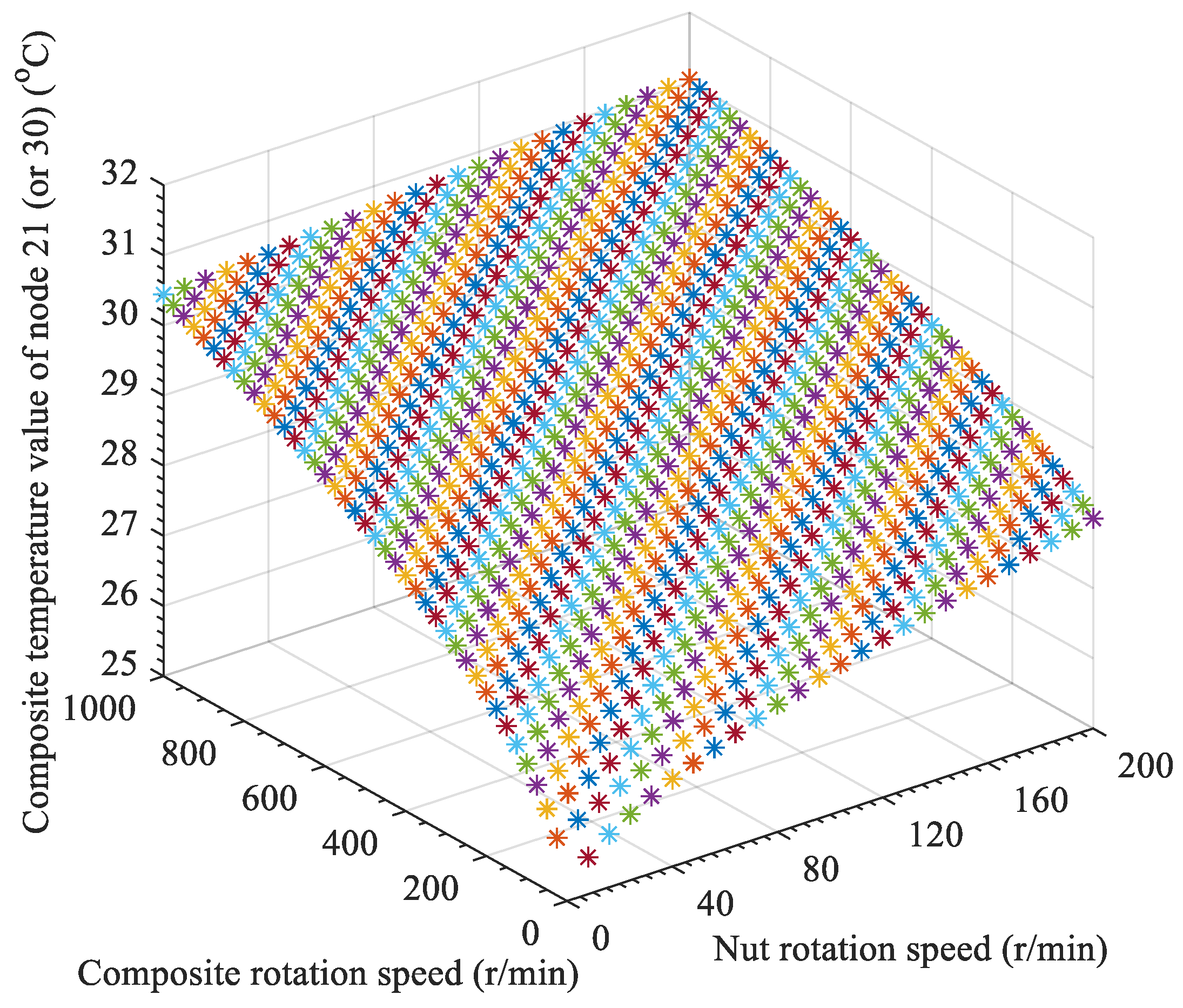
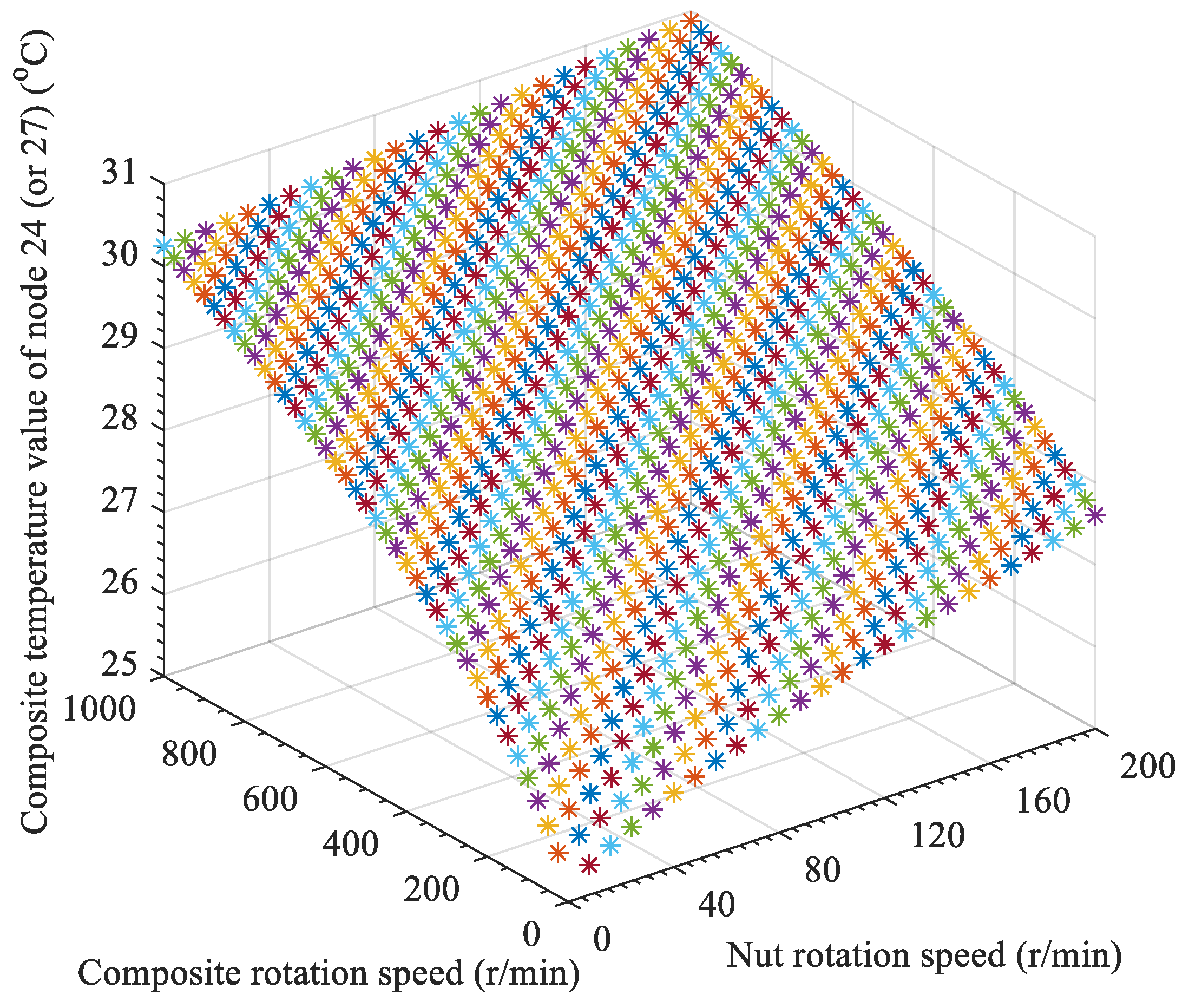
3.4. Node Synthesis Temperature of Nut-Rotating Ball Screw under Multiple Heat Source Working Conditions

Figure 21, Figure 22, Figure 23, Figure 24, Figure 25 and Figure 26 show the variation in node temperature values of the nut-rotating ball screw transmission mechanism under multiple heat source working conditions with variations in nut rotation speed and composite rotation speed. In line with the principle of linear superposition, the node temperature of the multiple heat sources is equal to the superposition of temperatures under the action of different single heat sources. Moreover, the composite temperature of the nodes is a prerequisite for addressing the thermal error of the screw.

When the nut rotation speed is $n_N=0\mathrm{RPM}$, the node temperature rises rapidly with the increasing screw speed. When the nut rotation speed and the composite rotation speed are $\Delta \ne 0\mathrm{RPM}$, under the same feed rate, the node temperature value under the dual-drive condition is higher than that under the single-drive condition. When the composite rotation speed is $\Delta =0\mathrm{RPM}$, the composite temperature of the nodes is much higher with the increasing nut (or screw) speed compared with the node temperature of the screw single drive at the same speed. The distribution of its temperature field is much more complex than the screw’s single-drive mechanism under the same parameters considering the unique transmission components and driving mode of the nut-rotating ball screw transmission mechanism.

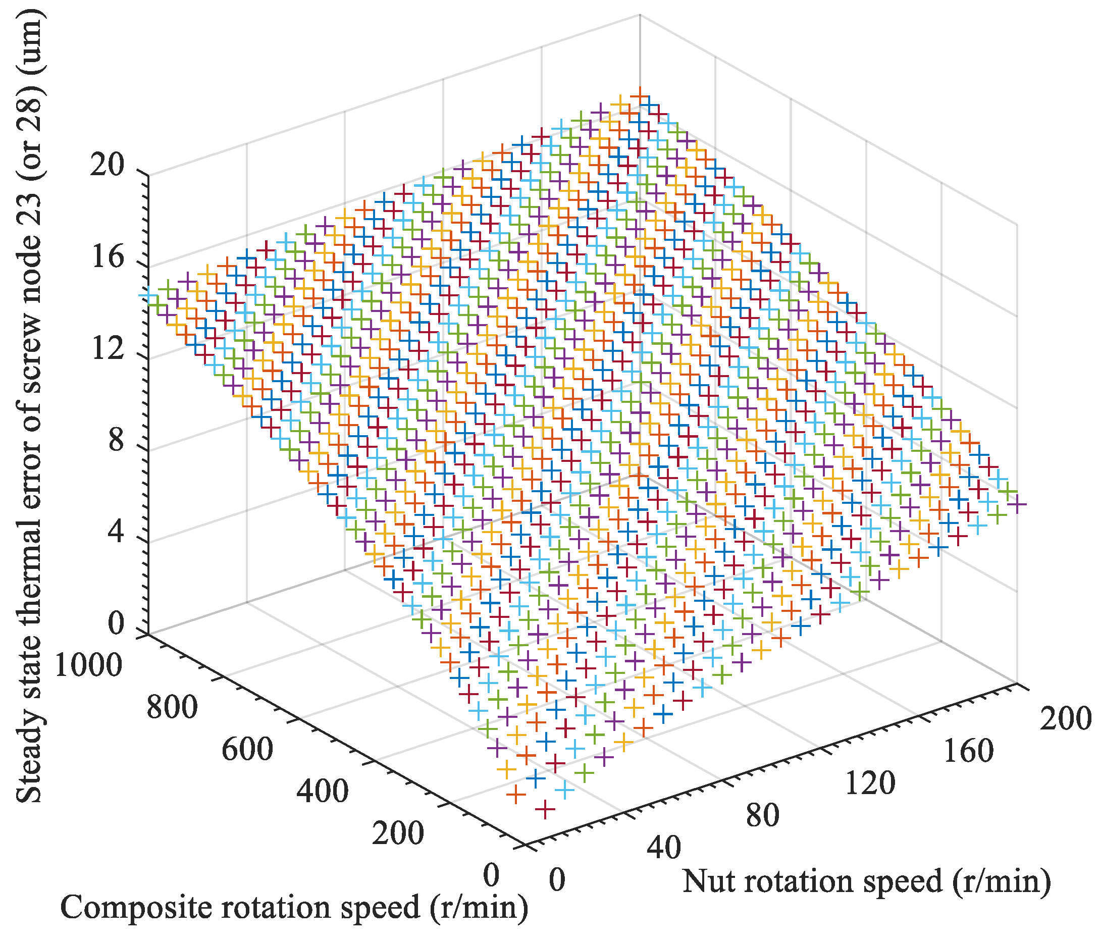
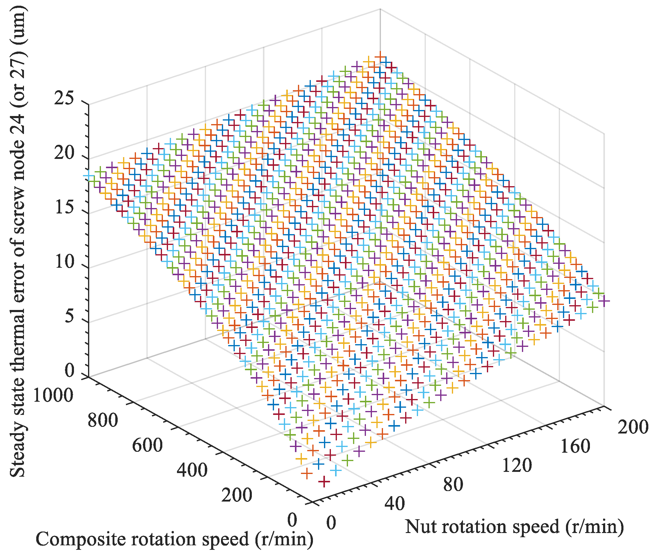
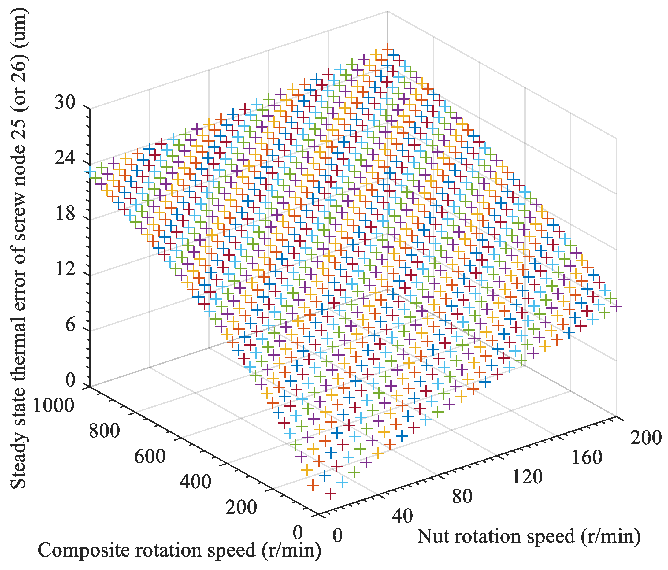
3.5. Steady State Thermal Error of Nut-Rotating Ball Screw

Figure 27, Figure 28, Figure 29, Figure 30, Figure 31 and Figure 32 display the steady-state thermal error of each node of the screw as a function of the nut rotation speed and the combined rotation speed. With the increasing distance from the fixed end of the screw, the steady-state thermal error of the screw also tends to increase. Because the steady-state thermal error of the screw can be obtained by integrating temperature with position, its value also increases with the increasing nut rotation speed and the composite rotation speed. The steady-state thermal error of each node under the dual-drive condition is greater than under the single-drive condition. Thermal deformation error is a vital component of motion error in micro-feed systems, and it is essential to consider research for precision feed control.

4. Temperature Rise and Thermal Elongation Testing Experiment for Nut-Rotating Ball Screw Transmission Mechanism

The temperature field distribution and thermal elongation exert a significant impact on the transmission accuracy of a feed system. Therefore, it is necessary to verify the established thermal resistance network model by experimentally measuring the temperature rise in the dual-drive feed system and the thermal elongation of the screw, providing a theoretical foundation for studying thermal error compensation.

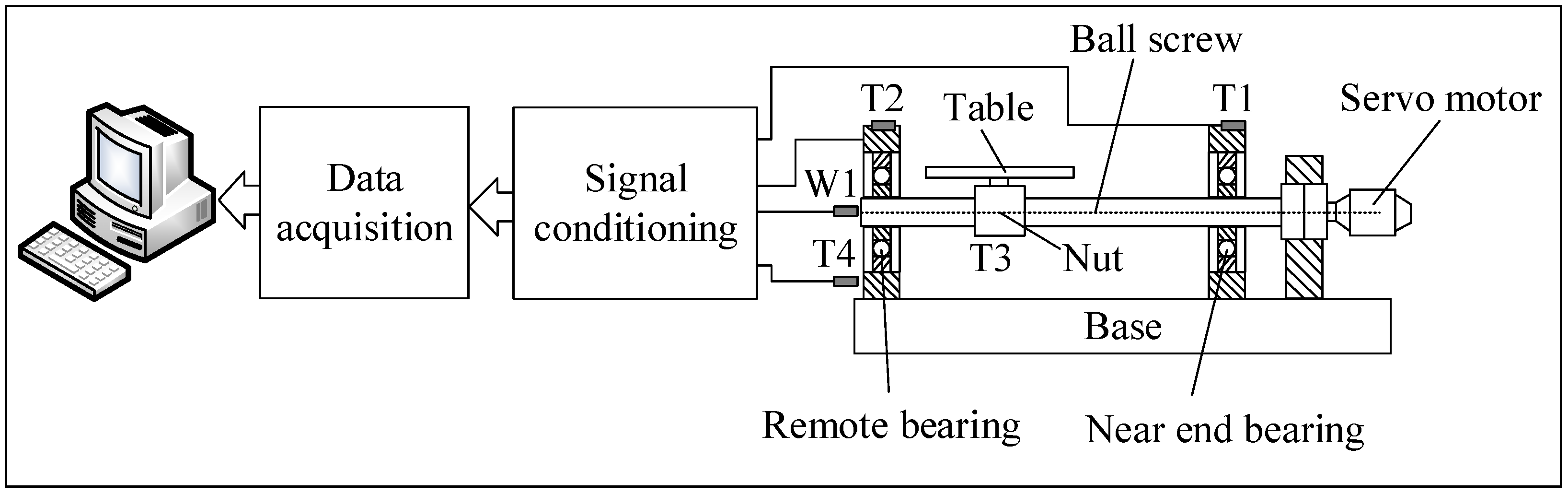
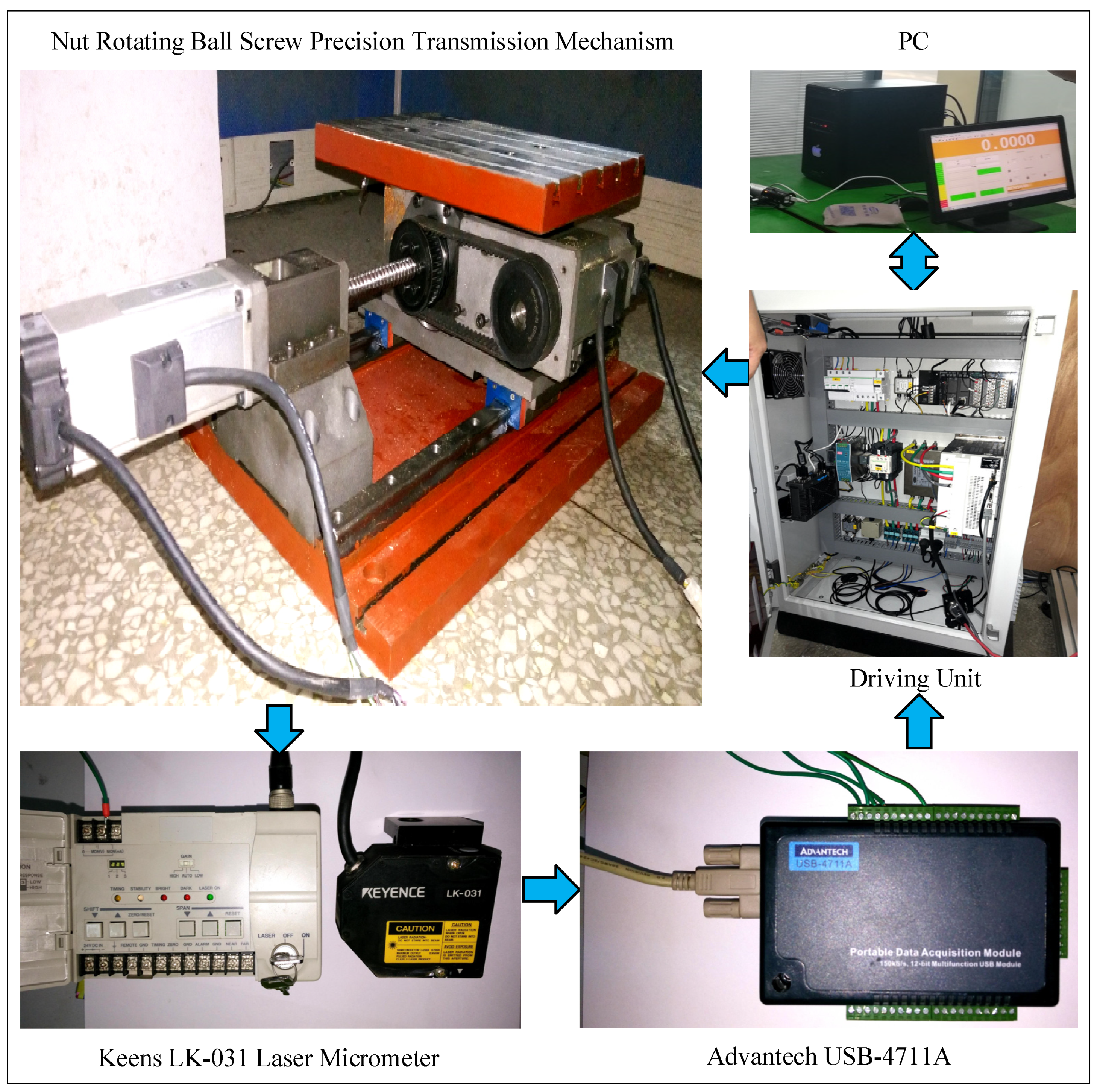
4.1. Construction of Temperature Rise and Thermal Elongation Testing System

Figure 33 presents a schematic of the testing scenario. In most cases, the hardware of the detection system consists of temperature sensors (T1, T2, T3, and T4), transmitters, data acquisition cards, micro-displacement sensors (W1), etc. To detect the temperature of the proximal bearing, temperature sensor T1 is installed near the screw motor bearing, while temperature sensor T2 is installed far away from the screw motor bearing to detect the temperature of the remote bearing; in addition, temperature sensor T3 is installed at the flange of the nut assembly to detect the temperature of the nut assembly and temperature sensor T4 is adopted to detect the ambient temperature. Micro-displacement sensor W1 employs the Keens LK-031 laser micrometer to measure axial thermal elongation at the end of the screw, with a maximum measurement length of 1 mm, a transmission output of −5~5 V, and a resolution of 0.1 $\mathsf{\mu }\mathrm{m}$.

Based on the temperature measurement requirements of the machine tool as well as the measurement range and accuracy requirements, the temperature sensor takes a Pt100 thermistor and a matching temperature transmitter, with a temperature measurement range of 0$°\mathrm{C}$–100$°\mathrm{C}$ and a transmission output of 0–5 V. An advantech USB-4711A multi-channel data acquisition card with 16 analog input channels, 12-bit resolution, and a maximum sampling rate of 150 k/s is selected.

Figure 34 presents the experimental setup. According to a previous publication by the author of this paper [33], the minimum speed of both motors is no less than 60 RPM, and the speed difference between the two is no less than 36 RPM to ensure the stable output speed of the dual-drive system table. During the temperature rise and thermal deformation experiment, the nut motor speed was set to 180 RPM, and the screw motor speed was set to 216 RPM. At this speed, the synthetic feed rate of the table was 3 $\mathrm{mm}/\mathrm{s}$. The dual-drive system was operated for a sufficient amount of time. The temperature increases at the near-end bearing of the screw motor, the far-end bearing of the screw motor, the flange of the nut component, and the thermal deformation at the end of the screw were detected through temperature sensors, transmitters, data acquisition cards, and micro displacement sensors.

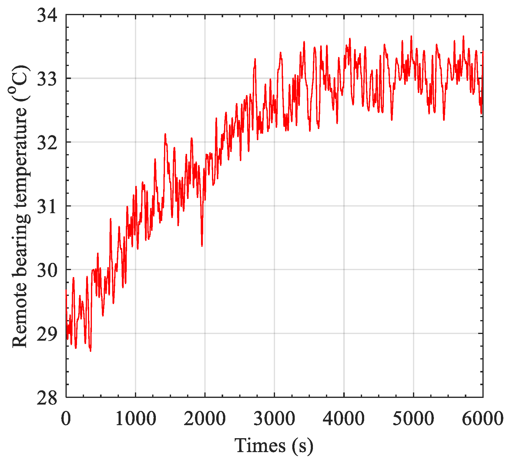
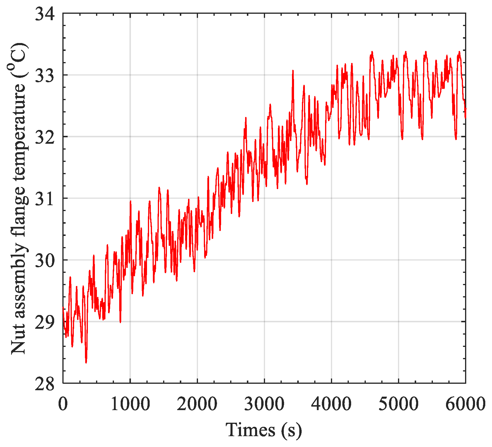
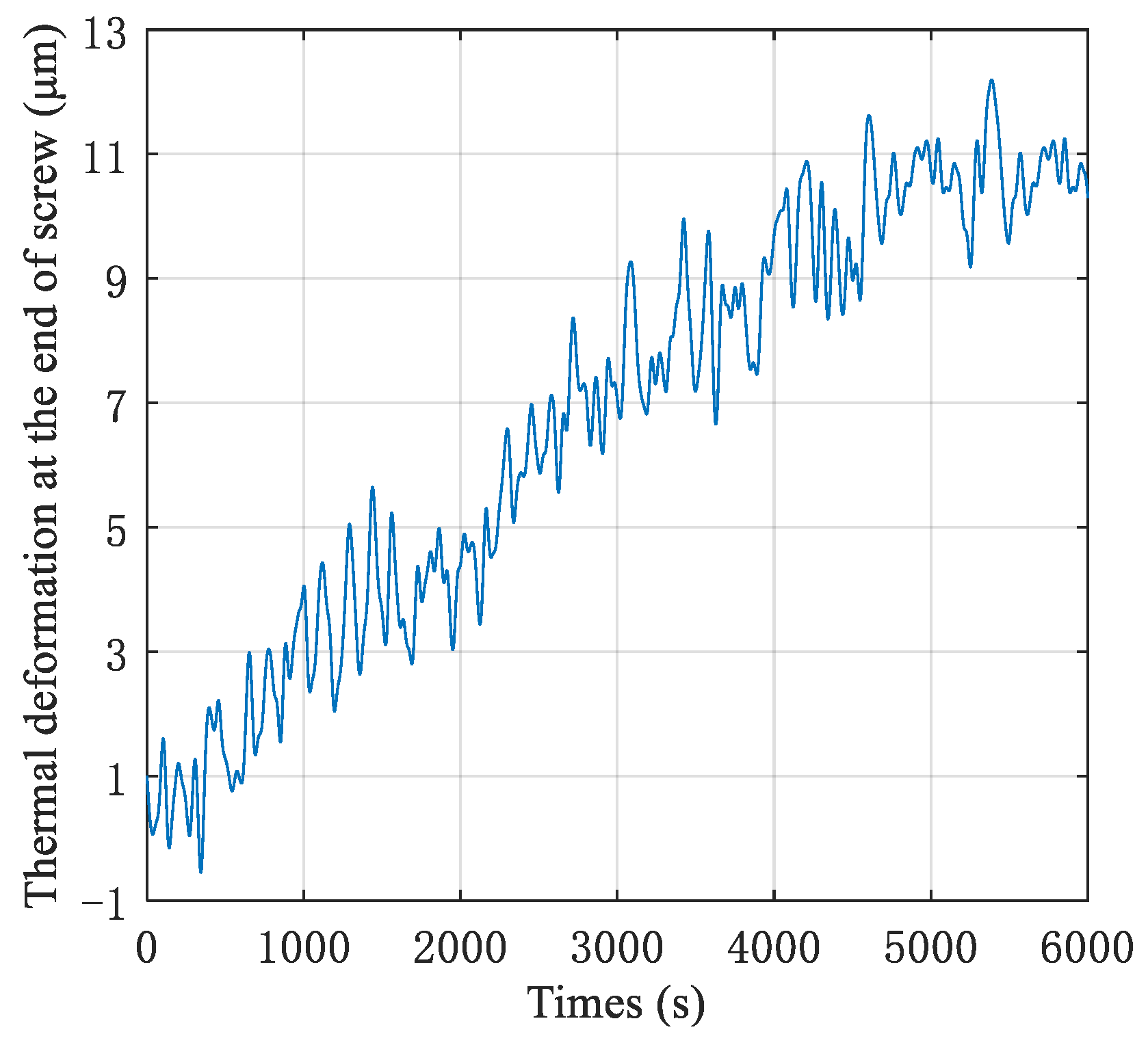
4.2. Experimental Results and Test Analysis

Figure 35, Figure 36 and Figure 37 present the temperature changes at the near-end bearing of the screw motor, the far-end bearing of the screw motor, and the flange of the nut assembly under the dual-drive condition, indicated by a nut speed of 180 RPM and a screw speed of 216 RPM. As per Figure 35, after running for a sufficient period, the near-end bearing of the screw motor reaches a thermal steady state. The experimentally measured temperature rise value is approximately 7.5$°\mathrm{C}$, and the simulated steady-state temperature rise value of the near-end bearing of the screw motor is 6.21 $°\mathrm{C}$. Figure 36 shows that the experimental temperature rise in the remote bearing of the screw motor after reaching thermal stability is approximately 4$°\mathrm{C}$, and the simulation shows that the steady-state temperature rise in the remote bearing of the screw motor is 3.2$°\mathrm{C}$. Figure 37 shows that the experimental temperature rise in the nut assembly flange after reaching thermal stability is about 3.8$°\mathrm{C}$, and the simulation demonstrates that the steady-state temperature increase in the nut assembly flange is 2.37$°\mathrm{C}$. The steady-state temperature rise experimental values obtained at the key points are consistent with the simulation results.

Figure 38 shows that the thermal elongation at the end of the screw was experimentally measured under the dual-drive condition. After reaching the thermal steady state, the measured thermal elongation at the end of the screw in the experiment is approximately 10.5 $\mathsf{\mu }\mathrm{m}$, and the simulation result is 11.98 $\mathsf{\mu }\mathrm{m}$. The experimental measurement result demonstrates the accuracy of the theoretical analysis model for thermal error at the end of the screw.

Through system temperature rise and thermal deformation experiments, it can be seen that the temperature field distribution of the nut-rotating ball screw transmission mechanism is much more complex than the traditional screw single-drive system, and the temperature rise is also more obvious. This phenomenon is mainly caused by the complex structure and unique driving method of the nut-rotating ball screw pair. In the nut assembly, friction heat is generated between the nut and the ball, with friction heat generation being integrated into the rolling bearing inside the nut assembly. Installing the nut assembly in a relatively narrow space is not conducive to heat dissipation, which can easily increase the system temperature and thermal deformation. In this study, the thermal network method is used to establish a thermodynamic model of a nut-rotating ball screw transmission mechanism. The correctness of the theoretical model is demonstrated through the experiments, which is important for improving the transmission accuracy of the system.

4.3. Thermal Effects Optimization Measures

The thermal deformation caused by temperature rise can affect the feed accuracy of the system, so the thermal effects of the system can be optimized and improved from the following three perspectives.

4.3.1. Reduce the Heat Generation of the System Heat Source

(1)

Using fewer intermediate transmission links to reduce the number of heat sources;

(2)

Using non-contact bearings, guide rails, and screws (such as hydraulic bearings, hydrostatic guide rails, and hydrostatic screws) or low-friction ceramic bearings;

(3)

Reasonably adjusting the pre-tightening force of the bearing and screw and supplementing with appropriate lubricants;

(4)

Improving the structure of the ball screw pair, such as by increasing the number of threaded heads, reducing the diameter of steel balls, using hollow balls, and improving the surface processing quality of the raceway.

4.3.2. Enhance the Cooling Capacity of the System

(1)

Using hollow ball screw pairs as transmission components and performing forced circulation cooling on the screw pairs and bearings;

(2)

Using oil–air micro-lubrication;

(3)

Set a constant temperature working environment.

4.3.3. Compensating for Thermal Errors in the Transmission System

(1)

Feedback interception method: By inserting a feedback loop into the servo system, thermal error compensation is achieved by adjusting the position of the tool holder;

(2)

Zero drift method: Calculating the compensation amount based on the established thermal error model and then sending it to the CNC controller. Finally, the compensation amount is added at each position as a command signal to the servo loop for feedforward compensation.

5. Conclusions

(1)

A thermal resistance network model of a nut-rotating ball screw transmission system was established based on heat transfer theory. By addressing the system’s thermal balance equations, the distribution of its temperature field was analyzed. The results objectively reflected the temperature distribution in the system. The temperature distribution of the entire system basically conforms to the law of heat flow, indicating that the use of the thermal resistance network method for temperature field analysis of the multi-heat source system is effective. The prediction accuracy of the model can be enhanced by arranging more temperature nodes and employing experimental data to identify and correct the model parameters.

(2)

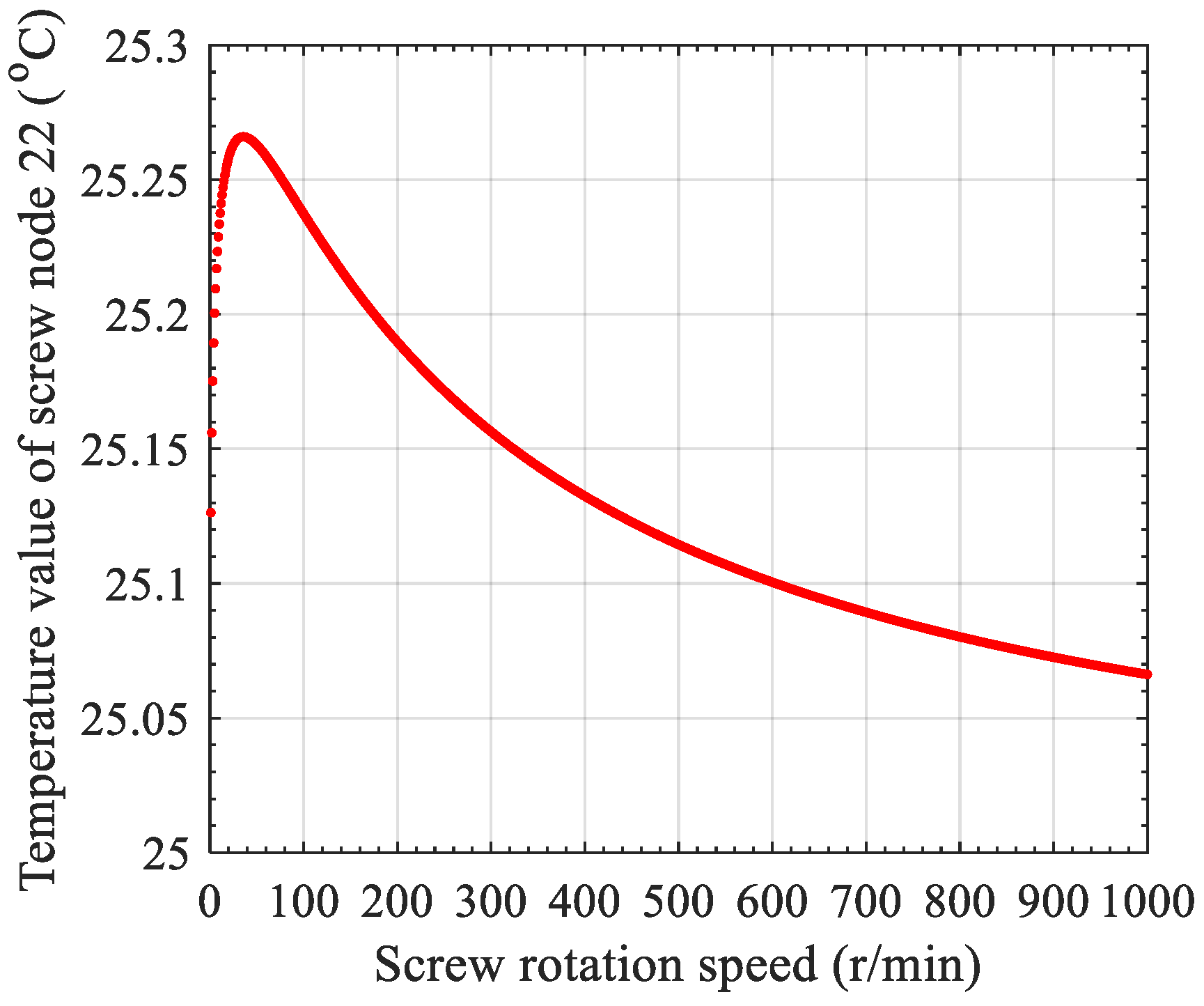
When a unilateral heat source functions, as the distance from the heat source point increases, the steady-state temperature value of the node rapidly decays. Under the condition that the screw speed reaches a certain value, there is a point where its temperature will maintain a thermal equilibrium state and not change with the increase in screw speed. At nodes far away from the heat source, the temperature is characterized by a slight increase followed by a decrease and tends towards the ambient temperature as the screw speed increases.

(3)

The outer ring supporting the bearing in the nut assembly is integrated with the flange in the nut assembly, and the inner ring supporting the bearing can be integrated with the outer ring of the rotating nut. In addition, the nut and screw are driven separately. Due to the proposed structure and driving method, the dual-drive mechanism has varying heat source points from the conventional mechanism, which are also the main factors causing the different heat source distributions of the dual-drive feed mechanism.

(4)

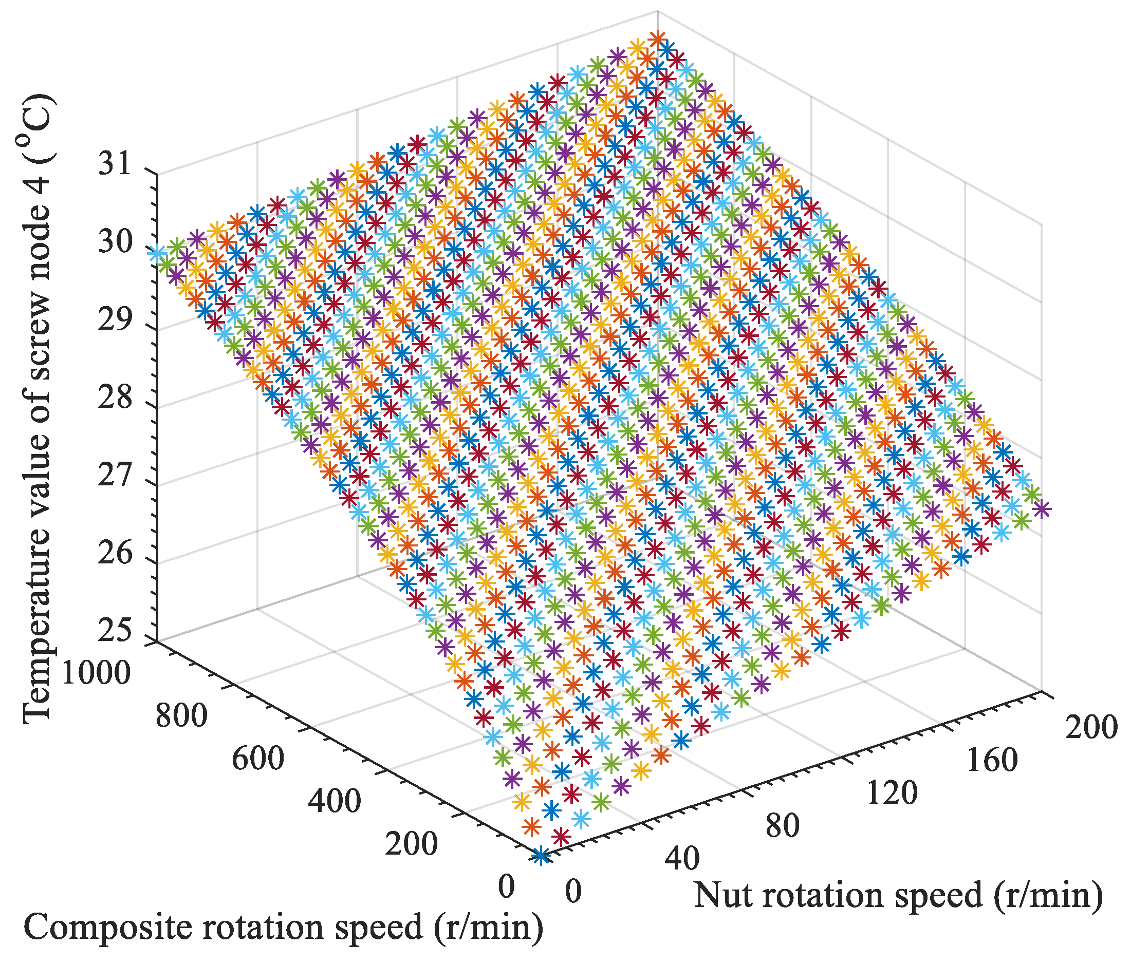
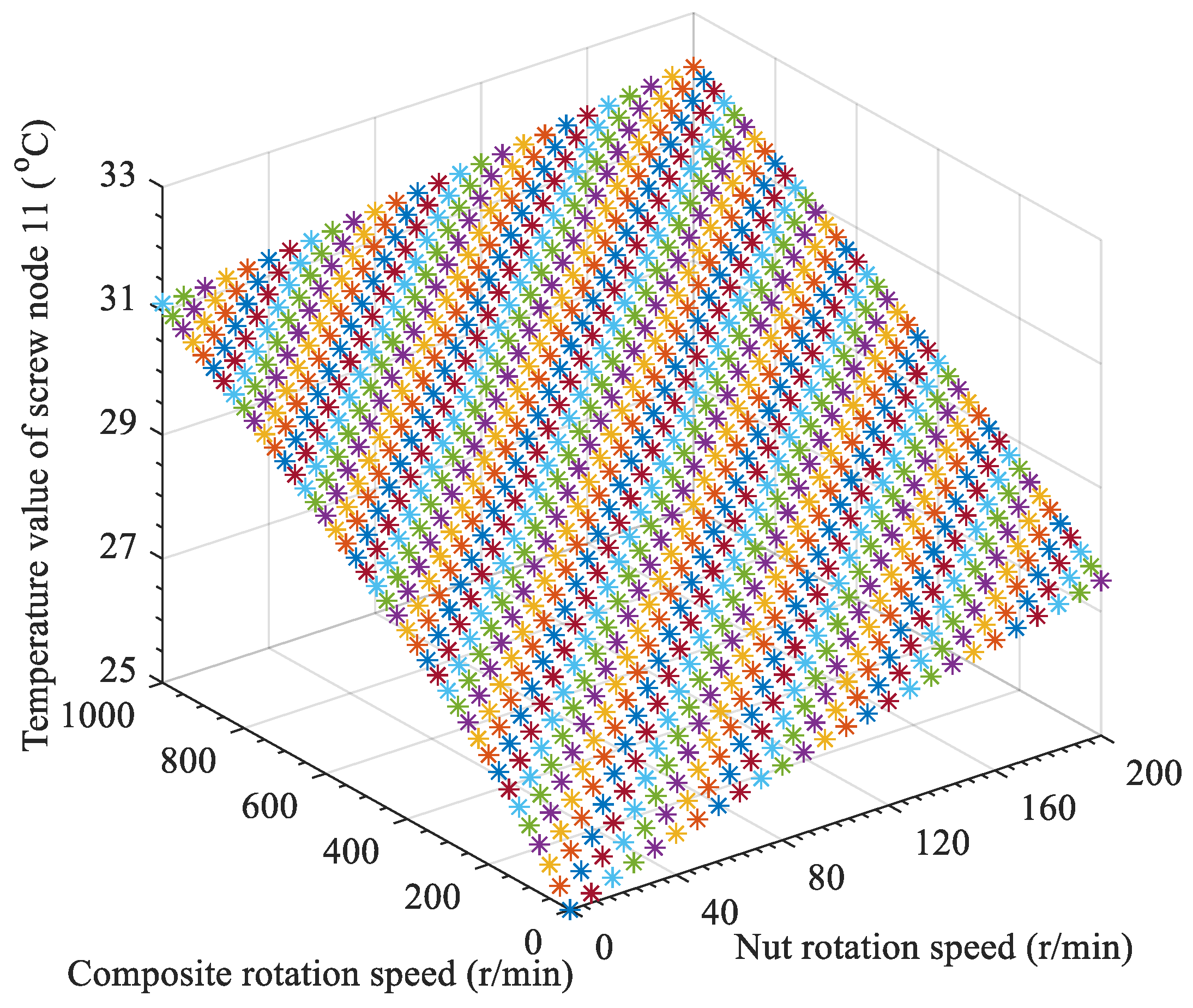
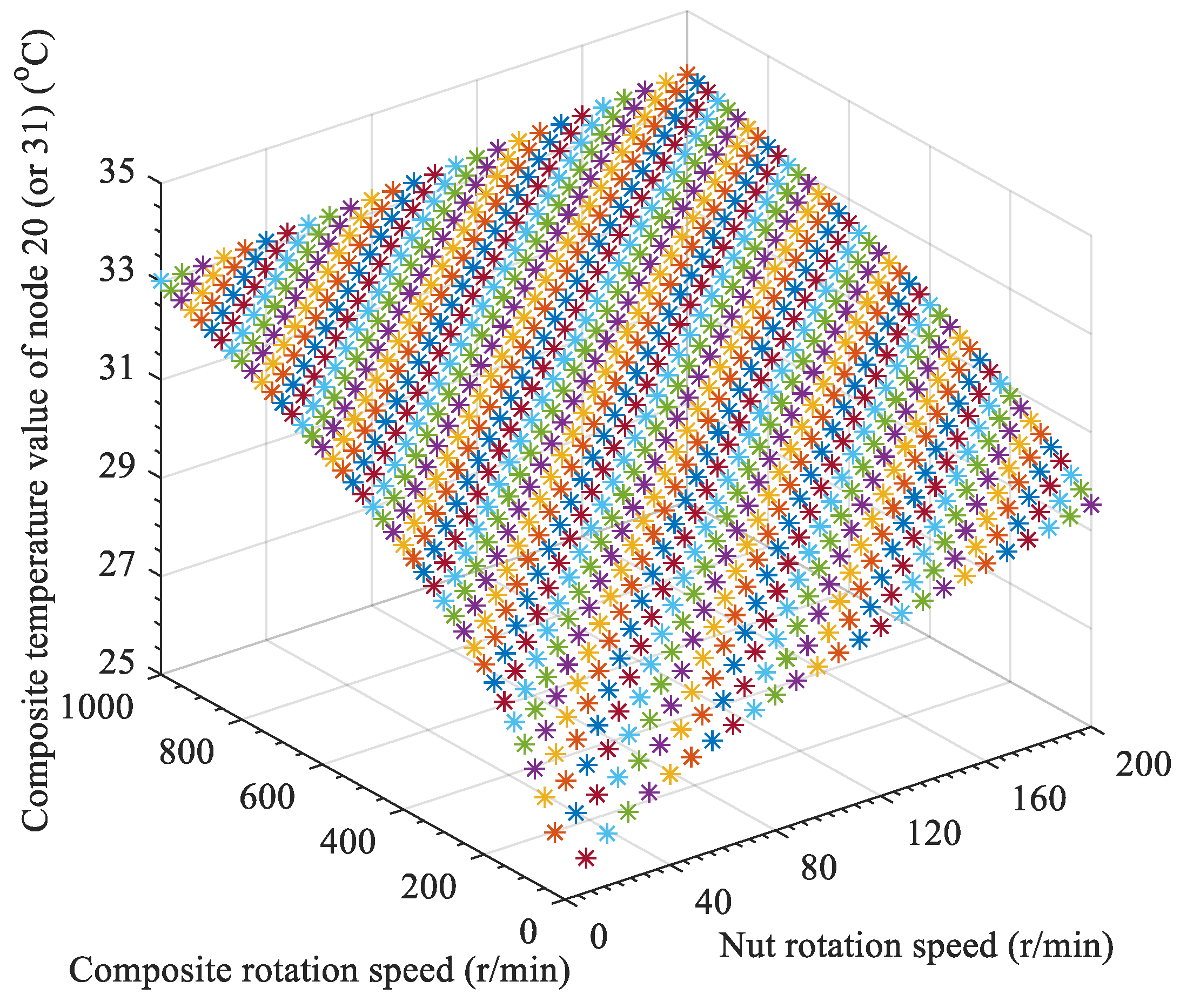
Under the action of multiple heat sources and the same feed rate, the node temperature value under the dual-drive condition is higher when compared with that under the single-drive condition, and the distribution of the temperature field is much more complex than that of the single-drive mechanism under the same parameters. Considering the fact that the steady-state thermal error of the screw can be acquired by integrating temperature with the position, the value of the steady-state thermal error also tends to increase with an increase in nut rotation speed and composite rotation speed. In addition, the steady-state thermal error of each node under the dual-drive condition is greater than that under the single-drive condition.

(5)

The potential applications of the nut rotary ball screw transmission mechanism and the results of numerical analysis can be applied to advanced technology fields such as robotics, suspensions, powertrain, national defense, integrated electronics, optoelectronics, medicine, and genetic engineering so that the new system can have a lower stable speed limit and achieve precise micro-feed control.

References

1. Delor, M.; Weaver, H.L.; Yu, Q.Q.; Ginsberg, N.S. Imaging material functionality through three-dimensional nanoscale tracking of energy flow. Nat. Mater. 2020, 19, 56–62. [Google Scholar] [CrossRef]
2. Li, Z.M.; Gao, X.Y.; Yang, J.K.; Xin, X.D.; Yi, X.Y.; Bian, L.; Dong, S.X. Designing Ordered Structure with Piezoceramic Actuation Units (OSPAU) for Generating Continual Nanostep Motion. Adv. Sci. 2020, 7, 2001155. [Google Scholar] [CrossRef]
3. Russo, M.; Zhang, D.; Liu, X.J.; Xie, Z.H. A review of parallel kinematic machine tools: Design, modeling, and applications. Int. J. Mach. Tools Manuf. 2024, 196, 104118. [Google Scholar] [CrossRef]
4. Weng, L.T.; Gao, W.G.; Zhang, D.W.; Huang, T.; Duan, G.L.; Liu, T.; Zheng, Y.J.; Shi, K. Analytical modelling of transient thermal characteristics of precision machine tools and real-time active thermal control method. Int. J. Mach. Tools Manuf. 2023, 186, 104003. [Google Scholar] [CrossRef]
5. Li, Y.; Yu, M.L.; Bai, Y.M.; Hou, Z.Y.; Wu, W.W. A review of thermal error modeling methods for machine tools. Appl. Sci. 2021, 11, 5216. [Google Scholar] [CrossRef]
6. Han, L.; Tong, Z.Y. A thermal resistance network model based on three-dimensional structure. Measurement 2019, 133, 439–443. [Google Scholar] [CrossRef]
7. Li, D.T.; He, Z.L.; Wang, C.; Sun, S.Z.; Ma, K.; Xing, Z.W. Simulation of dry screw vacuum pumps based on chamber model and thermal resistance network. Appl. Therm. Eng. 2022, 211, 118460. [Google Scholar] [CrossRef]
8. Sun, Z.H.; Xu, Y.F.; Wang, Q.J.; Xu, J.Z.; Li, G.L.; Wen, Y. Design and identification of lumped-parameter thermal network model for real-time temperature estimation of permanent-magnet spherical motors. Therm. Sci. Eng. Prog. 2023, 44, 102047. [Google Scholar] [CrossRef]
9. Meng, Q.Y.; Yan, X.X.; Sun, C.C.; Liu, Y. Research on thermal resistance network modeling of motorized spindle based on the influence of various fractal parameters. Int. Commun. Heat Mass Transf. 2020, 117, 104806. [Google Scholar] [CrossRef]
10. Zhu, Z.Y.; Zhang, W.; Li, Y.B.; Guo, J. Thermal analysis of axial permanent magnet flywheel machine based on equivalent thermal network method. IEEE Access 2021, 9, 33181–33188. [Google Scholar] [CrossRef]
11. Bao, Y.J.; Ma, Y.X.; Yang, Y.X.; Wang, J.L.; Cheng, D. Study on the effect of carbon fiber ply angle on thermal response of CFRP laminate based on the thermal resistance network model. Polym. Compos. 2023, 44, 8792–8804. [Google Scholar] [CrossRef]
12. Zhan, Z.Q.; Fang, B.; Wan, S.K.; Bai, Y.; Hong, J.; Li, X.H. An accurate and efficient implicit thermal network method for the steady-state temperature field. Proc. Inst. Mech. Eng. Part C J. Mech. Eng. Sci. 2024, 238, 1800–1810. [Google Scholar] [CrossRef]
13. Li, T.J.; Wang, M.Z.; Zhao, C.Y. Study on real-time thermal–mechanical–frictional coupling characteristics of ball bearings based on the inverse thermal network method. Proc. Inst. Mech. Eng. Part J J. Eng. Tribol. 2021, 235, 2335–2349. [Google Scholar] [CrossRef]
14. Yang, Y.B.; Zhou, X. A volumetric heat source model for thermal modeling of additive manufacturing of metals. Metals 2020, 10, 1406. [Google Scholar] [CrossRef]
15. Wu, H.Y.; Guan, Q.; Xi, C.F.; Zuo, D.W. Construction of dynamic temperature field model of ball screw based on superposition of positive and negative temperature fields. Numer. Heat Transf. Part A Appl. 2023, 83, 343–360. [Google Scholar] [CrossRef]
16. Liu, J.L.; Ma, C.; Wang, S.L.; Wang, S.B.; Yang, B.; Shi, H. Thermal boundary condition optimization of ball screw feed drive system based on response surface analysis. Mech. Syst. Signal Process. 2019, 121, 471–495. [Google Scholar] [CrossRef]
17. Sheng, X.; Lu, X.; Zhang, J.R.; Lu, Y.Q. An analytical solution to temperature field distribution in a thick rod subjected to periodic-motion heat sources and application in ball screws. Eng. Optim. 2021, 53, 2144–2163. [Google Scholar] [CrossRef]
18. Wang, L.; Jia, Z.Y.; Zhang, L. Investigation on the accurate calculation of the temperature field of permanent magnet governor and the optimization method of heat conduction. Case Stud. Therm. Eng. 2019, 13, 100360. [Google Scholar] [CrossRef]
19. Liu, W.Z.; Zhang, C.; Duan, F.J.; Fu, X.; Bao, R.J.; Yu, Z.X.; Gong, X. An optimization method of temperature field distribution to improve the accuracy of laser multi-degree-of-freedom measurement system. Optik 2022, 269, 169721. [Google Scholar] [CrossRef]
20. Sun, S.B.; Yan, S.H.; Cao, X.P.; Zhang, W. Distribution law of the initial temperature field in a railway tunnel with high rock temperature: A model test and numerical analysis. Appl. Sci. 2023, 13, 1638. [Google Scholar] [CrossRef]
21. Gao, X.S.; Zhang, K.; Zhang, Z.T.; Wang, M.; Zan, T.; Gao, P. XGBoost-based thermal error prediction and compensation of ball screws. Proc. Inst. Mech. Eng. Part B J. Eng. Manuf. 2024, 238, 151–163. [Google Scholar] [CrossRef]
22. Su, D.X.; Li, Y.; Zhao, W.H.; Zhang, H.J. Transient thermal error modeling of a ball screw feed system. Int. J. Adv. Manuf. Technol. 2023, 124, 2095–2107. [Google Scholar] [CrossRef]
23. Yang, J.C.; Li, C.Y.; Xu, M.T.; Zhang, Y.M. Analysis of thermal error model of ball screw feed system based on experimental data. Int. J. Adv. Manuf. Technol. 2022, 119, 7415–7427. [Google Scholar] [CrossRef]
24. Li, Y.; Fan, J.B.; Zheng, Y.N.; Gao, F.; Li, W.Q.; Hei, C.F. Thermal error compensation for a fluid-cooling ball-screw feed system. Proc. Inst. Mech. Eng. Part B J. Eng. Manuf. 2024, 09544054231210963. [Google Scholar] [CrossRef]
25. Liu, H.L.; Rao, Z.F.; Pang, R.D.; Zhang, Y.M. Research on thermal characteristics of ball screw feed system considering nut movement. Machines 2021, 9, 249. [Google Scholar] [CrossRef]
26. Shi, H.; Ma, C.; Yang, J.; Zhao, L.; Mei, X.S.; Gong, G.F. Investigation into effect of thermal expansion on thermally induced error of ball screw feed drive system of precision machine tools. Int. J. Mach. Tools Manuf. 2015, 97, 60–71. [Google Scholar] [CrossRef]
27. Rong, R.; Zhou, H.C.; Huang, Y.B.; Yang, J.Z.; Xiang, H. Novel Real-Time Compensation Method for Machine Tool’s Ball Screw Thermal Error. Appl. Sci. 2023, 13, 2833. [Google Scholar] [CrossRef]
28. Cao, L.; Park, C.H.; Chung, S.C. Real-time thermal error prediction and compensation of ball screw feed systems via model order reduction and hybrid boundary condition update. Precis. Eng.-J. Int. Soc. Precis. Eng. Nanotechnol. 2022, 77, 227–240. [Google Scholar] [CrossRef]
29. Tanaka, S.; Kizaki, T.; Tomita, K.; Tsujimura, S.; Kobayashi, H.; Sugita, N. Robust thermal error estimation for machine tools based on in-process multi-point temperature measurement of a single axis actuated by a ball screw feed drive system. J. Manuf. Process. 2023, 85, 262–271. [Google Scholar] [CrossRef]
30. Liu, H.Y.; Deng, H.G.; Feng, X.Y.; Liu, Y.D.; Li, Y.F.; Yao, M. Data-driven thermal error modeling based on a novel method of temperature measuring point selection. Int. J. Adv. Manuf. Technol. 2024, 131, 1823–1848. [Google Scholar] [CrossRef]
31. Peng, J.; Yin, M.; Cao, L.; Liao, Q.H.; Wang, L.; Yin, G.F. Study on the spindle axial thermal error of a five-axis machining center considering the thermal bending effect. Precis. Eng. 2022, 75, 210–226. [Google Scholar] [CrossRef]
32. Yu, H.W.; Feng, X.Y.; Sun, Q. Kinematic analysis and simulation of a new type of differential micro-feed mechanism with friction. Sci. Prog. 2020, 103, 0036850419875667. [Google Scholar] [CrossRef] [PubMed]
33. Yu, H.W.; Zhang, L.G.; Wang, C.; Feng, X.Y. Dynamic characteristics analysis and experimental of differential dual drive servo feed system. Proc. Inst. Mech. Eng. Part C J. Mech. Eng. Sci. 2021, 235, 6737–6751. [Google Scholar] [CrossRef]
Figure 1. Nut rotating ball screw precision transmission mechanism.
Applsci 14 05790 g001
Figure 2. Schematic diagram of heat source distribution in the transmission system.
Applsci 14 05790 g002
Figure 3. Heat transfer circuit diagram of the dual-drive nut-rotating ball screw pair.
Applsci 14 05790 g003
Figure 4. Temperature node layout diagram of the dual-drive nut-rotating ball screw pair.
Applsci 14 05790 g004
Figure 5. Layout diagram of the screw temperature nodes for the left-bearing heat source.
Applsci 14 05790 g005
Figure 6. Layout diagram of the screw temperature nodes for the right-bearing heat source.
Applsci 14 05790 g006
Figure 7. Thermal resistance network model of the dual-drive nut-rotating ball screw pair.
Applsci 14 05790 g007
Figure 8. Thermal network model of the screw under the action of the screw’s left-bearing heat source.
Applsci 14 05790 g008
Figure 9. Thermal network model of the screw under the action of the screw’s right-bearing heat source.
Applsci 14 05790 g009
Figure 10. Schematic diagram of the thermal error of the screw.
Applsci 14 05790 g010
Figure 11. Temperature value of screw node 19 under single heat source.
Applsci 14 05790 g011
Figure 12. Temperature value of screw node 20 under single heat source.
Applsci 14 05790 g012
Figure 13. Temperature value of screw node 21 under single heat source.
Applsci 14 05790 g013
Figure 14. Temperature value of screw node 22 under single heat source.
Applsci 14 05790 g014
Figure 15. Temperature value of screw node 23 under single heat source.
Applsci 14 05790 g015
Figure 16. Temperature value of screw node 24 under single heat source.
Applsci 14 05790 g016
Figure 17. Temperature value of screw node 4 under single heat source.
Applsci 14 05790 g017
Figure 18. Temperature value of screw node 8 under single heat source.
Applsci 14 05790 g018
Figure 19. Temperature value of screw node 10 under single heat source.
Applsci 14 05790 g019
Figure 20. Temperature value of screw node 11 under single heat source.
Applsci 14 05790 g020
Figure 21. Synthetic temperature value of screw node 20 (or 31) under multiple heat sources.
Applsci 14 05790 g021
Figure 22. Synthetic temperature value of screw node 21 (or 30) under multiple heat sources.
Applsci 14 05790 g022
Figure 23. Synthetic temperature value of screw node 22 (or 29) under multiple heat sources.
Applsci 14 05790 g023
Figure 24. Synthetic temperature value of screw node 23 (or 28) under multiple heat sources.
Applsci 14 05790 g024
Figure 25. Synthetic temperature value of screw node 24 (or 27) under multiple heat sources.
Applsci 14 05790 g025
Figure 26. Synthetic temperature value of screw node 25 (or 26) under multiple heat sources.
Applsci 14 05790 g026
Figure 27. Steady-state thermal error of screw node 20 (or 31).
Applsci 14 05790 g027
Figure 28. Steady-state thermal error of screw node 21 (or 30).
Applsci 14 05790 g028
Figure 29. Steady-state thermal error of screw node 22 (or 29).
Applsci 14 05790 g029
Figure 30. Steady-state thermal error of screw node 23 (or 28).
Applsci 14 05790 g030
Figure 31. Steady-state thermal error of screw node 24 (or 27).
Applsci 14 05790 g031
Figure 32. Steady-state thermal error of screw node 25 (or 26).
Applsci 14 05790 g032
Figure 33. Schematic of the testing scenario.
Applsci 14 05790 g033
Figure 34. Experimental setup.
Applsci 14 05790 g034
Figure 35. Temperature of the screw motor near end bearing under dual-drive condition.
Applsci 14 05790 g035
Figure 36. Temperature of the screw motor remote end bearing under dual-drive condition.
Applsci 14 05790 g036
Figure 37. Temperature of the nut assembly flange under dual-drive condition.
Applsci 14 05790 g037
Figure 38. Thermal elongation at the end of the screw under dual-drive condition.
Applsci 14 05790 g038